Adaptive Fourier-Galerkin Methods
Abstract
We study the performance of adaptive Fourier-Galerkin methods in a
periodic box in with dimension . These methods offer
unlimited approximation power only restricted by solution and data
regularity. They are of intrinsic interest but are also a first step
towards understanding adaptivity for the -FEM.
We examine two nonlinear approximation classes, one
classical corresponding to algebraic decay of Fourier coefficients
and another associated with
exponential decay. We study the sparsity classes of the residual and
show that they are the same as the solution for the algebraic class but
not for the exponential one. This possible sparsity degradation for
the exponential class can be
compensated with coarsening, which we discuss in detail. We present
several adaptive Fourier algorithms, and prove their contraction
and optimal cardinality properties.
Keywords: Spectral methods, adaptivity, convergence, optimal cardinality.
a Dipartimento di Scienze Matematiche, Politecnico di Torino
Corso Duca degli Abruzzi 24, 10129 Torino, Italy
E-mail: claudio.canuto@polito.it
Department of Mathematics and Institute for Physical Science
and Technology,
University of Maryland, College Park, MD 20742, USAy
E-mail: rhn@math.umd.edu
c MOX, Dipartimento di Matematica, Politecnico di Milano
Piazza Leonardo da Vinci 32, I-20133 Milano, Italy
E-mail: marco.verani@polimi.it
1 Introduction
Adaptivity is now a fundamental tool in scientific and engineering computation. In contrast to the practice, which goes back to the 70’s, the mathematical theory for multidimensional problems is rather recent. It started in 1996 with the convergence results by Dörfler [13] and Morin, Nochetto, and Siebert [18]. The first convergence rates were derived by Cohen, Dahmen, and DeVore [7] for wavelets in any dimensions , and for finite element methods (AFEM) by Binev, Dahmen, and DeVore [2] for and Stevenson [21] for any . The most comprehensive results for AFEM are those of Cascón, Kreuzer, Nochetto, and Siebert [6] for any and data, and Cohen, DeVore, and Nochetto [8] for and data; we refer to the survey [19] by Nochetto, Siebert and Veeser. This theory is quite satisfactory in that it shows that AFEM delivers a convergence rate compatible with that of the approximation classes where the solution and data belong. The recent results in [8] reveal that it is the approximation class of the solution that really matters. In all cases though the convergence rates are limited by the approximation power of the method (both wavelets and FEM), which is finite and related to the polynomial degree of the basis functions, and the regularity of the solution and data. The latter is always measured in an algebraic approximation class.
In contrast very little is known for methods with infinite approximation power, such as those based on Fourier analysis. We mention here the results of DeVore and Temlyakov [12] for trigonometric sums and those of Binev et al [1] for the reduced basis method. A close relative to Fourier methods is the so-called -version of the FEM (see e.g. [20] and [5]), which uses Legendre polynomials instead of exponentials as basis functions. The purpose of this paper is to present adaptive Fourier-Galerkin methods (ADFOUR), and discuss their convergence and optimality properties. We do so in the context of both algebraic and exponential approximation classes, and take advantage of the orthogonality inherent to complex exponentials. We believe that this approach can be extended to the -FEM. We view this theory as a first step towards understanding adaptivity for the -FEM, which combines mesh refinement (-FEM) with polynomial enrichment (-FEM) and is much harder to analyze.
Our investigation reveals some striking differences between ADFOUR and AFEM and wavelet methods. The basic assumption, underlying the success of adaptivity, is that the information read in the residual is quasi-optimal for either mesh design or choosing wavelet coefficients for the actual solution. This entails that the sparsity classes of the residual and the solution coincide. We briefly illustrate below, and fully discuss later in Sect. 5, that this basic premise is false for exponential classes even though it is true for algebraic classes. Confronted with this unexpected fact, we have no alternative but to implement and study ADFOUR with coarsening for the exponential case; see Sect. 6 and Sect. 8. This was the original idea of Cohen et al [7] and Binev et al [2] for the algebraic case, but it was subsequently removed by Stevenson [21].
We give now a brief description of the essential issues we are confronted with in designing and studying ADFOUR. To this end, we assume that we know the Fourier representation of a periodic function , and its non-increasing rearrangement , namely, for all .
Dörfler marking and best -term approximation. We recall the marking introduced by Dörfler [13], which is the only one for which there exist provable convergence rates. Given a parameter , and a current set of Fourier frequencies or indices , say the first ones according to the labeling of , we choose the next set as the minimal set for which
| (1.1) |
where is the residual and is the orthogonal projection in the -norm onto . Note that, if and , then (1.1) can be equivalently written as
| (1.2) |
and that where is the complement of and likewise for . This is the simplest possible scenario because the information built in is exactly that of . Moreover, is the best -term approximation of in the -norm and the corresponding error is given by
| (1.3) |
Algebraic vs exponential decay. Suppose now that has the precise algebraic decay111Throughout the paper, means for some constant independent of the relevant parameters in the inequality; means .
| (1.4) |
with
| (1.5) |
and . We denote by the smallest constant in the upper bound in (1.4). We thus have
This decay is related to certain Besov regularity of [12]. Note that the effect of Dörfler marking (1.2) is to reduce the residual from to by a factor , or equivalently
with . Since the set is minimal, we deduce that , whence
| (1.6) |
for small enough. This means that the number of degrees of freedom to be added is proportional to the current number. This simplifies considerably the complexity analysis since every step adds as many degrees of freedom as we have already accumulated.
The exponential case is quite different. Suppose that has a genuinely exponential decay
| (1.7) |
corresponding to analytic functions [14], and let be the smallest constant appearing in the upper bound in (1.7). These definitions are slight simplifications of the actual ones in Sect. 4.3 but enough to give insight on the main issues at stake. We thus have
this and similar decays are related to Gevrey classes of functions [14]. In contrast to (1.6), Dörfler marking now yields222Throughout the paper, means for some quantity .
| (1.8) |
This shows that the number of additional degrees of freedom per step is fixed and independent of , which makes their counting as well as their implementation a very delicate operation.
Plateaux. We now consider a situation opposite to the ideal decay examined above. Suppose that the first Fourier coefficients of are constant and either
| (1.9) |
for each approximation class. A simple calculation reveals that either
| (1.10) |
Repeating the argument leading to (1.6) and (1.8) with , we infer that either
| (1.11) |
For this is a much larger number than the optimal values (1.6) and (1.8), and illustrates the fact that the Dörfler condition (1.1) adds many more frequencies in the presence of plateaux. We note that is a multiplicative constant in the left of (1.11) and additive in the right of (1.11).
Sparsity of the residual. In practice we do not have access to the Fourier decomposition of but rather of the residual , where is the forcing function and the differential operator. Only an operator with constant coefficients leads to a spectral representation with diagonal matrix , in which case the components of the residual are directly those of and . In general decays away from the main diagonal with a law that depends on the regularity of the coefficients of ; we will examine in Sect. 2.4 either algebraic or exponential decay. In this much more intricate and interesting endeavor, studied in this paper, the components of interact with entries of to give rise to . The question whether belongs to the same approximation class of thus becomes relevant because adaptivity decisions are made with , and thereby on the range of rather than its domain.
We now provide insight on the key issues at stake via a couple of heuristic examples; we discuss this fully in Sect. 5.1 and Sect. 5.2. We start with the exponential case: let be defined by
for a given integer and . This sequence exhibits gaps of size between consecutive nonzero entries for . Its non-decreasing rearrangement is thus given by
whence with . Let be the Toeplitz bi-infinite matrix given by
with . This matrix has main nontrivial diagonals and is both of exponential and algebraic class according to the Definition 2.1 below. The product is much less sparse than but, because , consecutive frequencies of do not interact with each other: the -th component reads
or otherwise. The non-decreasing rearrangement of becomes
Consequently, writing and observing that
and the equality is attained for , we deduce
We thus conclude that the action of may shift the exponential class, from the one characterized by the parameter for to the one characterized by for . This uncovers the crucial feature that the image of may be substantially less sparse than itself. In Sect. 5.2 we present a rigorous construction with decreasing exponentially from the main diagonal and another, rather sophisticated, construction that illustrates the fact that the exponent in the bound for may deteriorate to some in the corresponding bound for .
It is remarkable that a similar construction for the algebraic decay would not lead to a change of algebraic class. In fact, let be given by
and otherwise. The non-decreasing rearrangement of satisfies whence
On the other hand, the -th component of reads
or otherwise. The non-decreasing rearrangement of in turn satisfies
whence writing and arguing as before we infer that
Since we realize that is less sparse than but, in contrast to the exponential case, they belong to the same algebraic class . Moreover, we will prove later in Sect. 5.1 that preserves the class provided entries of possess a suitable algebraic decay away from the main diagonal.
Since Dörfler marking is applied to the residual , it is its sparsity class that determines the degrees of freedom to be added. The same argument leading to either (1.6) or (1.8) gives
for each class. We thus see that the ratios and control the behavior of the adaptive procedure. This has already been observed and exploited by Cohen et al [7] in the context of wavelet methods for the class . Our estimates, discussed in Sect. 5, are valid for both classes and use specific decay properties of the entries of .
Coarsening. Ever since its inception by Cohen et al [7] and Binev et al [2], this has been a controvertial issue for elliptic PDE. It was originally due to the lack of control on the ratio for large [7]. It was removed by Stevenson et al [16, 21] for the algebraic class via a clever argument that exploits the minimality of Dörfler marking. This implicitly implies that the approximation classes for both and coincide, which we prove explicitly in Sect. 5.1 for the algebraic case. This is not true though for the exponential case and is discussed in Sect. 5.2. For the latter, we need to resort to coarsening to keep the cardinality of ADFOUR quasi-optimal. To this end, we construct an insightful example in Sect. 6 and prove a rather simple but sharp coarsening estimate which improves upon [7].
Contraction constant. It is well known that the contraction constant cannot be arbitrarily close to for estimators whose upper and lower constants, , do not coincide. This is, however, at odds with the philosophy of spectral methods which are expected to converge superlinearly (typically exponentially). Assuming that the decay properties of are known, we can enrich Dörfler marking in such a way that the contraction factor becomes
This leads to as close to as desired and to aggressive versions of ADFOUR discussed in Sect. 3.
This paper can be viewed as a first step towards understanding adaptivity for the -FEM. However, the results we present are of intrinsic interest and of value for periodic problems with high degree of regularity and rather complex structure. One such problem is turbulence in a periodic box. Our techniques exploit periodicity and orthogonality of the complex exponentials, but many of our assertions and conclusions extend to the non-periodic case for which the natural basis functions are Legendre polynomials; this is the case of the -FEM. In any event, the study of adaptive Fourier-Galerkin methods seems to be a new paradigm in adaptivity, with many intriguing questions and surprises, some discussed in this paper. In contrast to the -FEM, they exhibit unlimited approximation power which is only restricted by solution and data regularity.
We organize the paper as follows. In Sect. 2 we introduce the Fourier-Galerkin method, present a posteriori error estimators, and discuss properties of the underlying matrix for both algebraic and exponential approximation classes. In Sect. 3 we deal with four algorithms, two for each class, and prove their contraction properties. We devote Sect. 4 to nonlinear approximation theory with an emphasis on the exponential class. In Sect. 5 we turn to the study of the sparsity classes for the residual along the lines outlined above. We examine the role of coarsening and prove a sharp coarsening estimate in Sect. 6. We conclude with optimality properties of ADFOUR for the algebraic class in Sect. 7 and for the exponential class in Sect. 8.
2 Fourier-Galerkin approximation
2.1 Fourier basis and norm representation
For , we consider , and the trigonometric basis
which is orthonormal in ; let
be the expansion of any and the representation of its norm via the Parseval identity. Let , and let be its dual. Since the trigonometric basis is orthogonal in as well, one has for any
| (2.1) |
here and in the sequel, denotes the Euclidean norm of the multi-index . On the other hand, if , we set
the norm representation is
| (2.2) |
Throughout the paper, we will use the notation to indicate both the -norm of a function , or the -norm of a linear form ; the specific meaning will be clear from the context.
Given any finite index set , we define the subspace of
we set , so that . If admits an expansion (converging in an appropriate norm), then we define its projection upon by setting
2.2 Galerkin discretization and residual
We now consider the elliptic problem
| (2.3) |
where and are sufficiently smooth real coefficients satisfying and in ; let us set
We formulate this problem variationally as
| (2.4) |
where (bar indicating as usual complex conjugate). We denote by the energy norm of any , which satisfies
| (2.5) |
Given any finite set , the Galerkin approximation is defined as
| (2.6) |
For any , we define the residual
Then, the previous definition of is equivalent to the condition
| (2.7) |
On the other hand, by the continuity and coercivity of the bilinear form , one has
| (2.8) |
or, equivalently,
| (2.9) |
2.3 Algebraic representations
Let us identify the solution of Problem (2.4) with the vector of its -normalized Fourier coefficients, where we set for convenience . Similarly, let us identify the right-hand side with the vector of its -normalized Fourier coefficients. Finally, let us introduce the bi-infinite, Hermitian and positive-definite matrix
| (2.10) |
Then, Problem (2.4) can be equivalently written as
| (2.11) |
We observe that the orthogonality properties of the trigonometric basis implies that the matrix is diagonal if and only if the coefficients and are constant in .
Next, consider the Galerkin problem (2.6) and let be the vector collecting the coefficients of indexed in ; let be the analogous restriction for the vector of the coefficients of . Finally, denote by the matrix that restricts a bi-infinite vector to the portion indexed in , so that is the corresponding extension matrix. Then, setting
| (2.12) |
Problem (2.6) can be equivalently written as
| (2.13) |
2.4 Properties of the stiffness matrix
It is useful to express the elements of in terms of the Fourier coefficients of the operator coefficients and . Precisely, writing and and using the orthogonality of the Fourier basis, one easily gets
| (2.14) |
Note that the diagonal elements are uniformly bounded from below,
| (2.15) |
whereas all elements are bounded in modulus by the elements of a Toeplitz matrix,
| (2.16) |
which decay as at a rate dictated by the smoothness of the operator coefficients. Indeed, if and are sufficiently smooth, their Fourier coefficients decay at a suitable rate and this property is inherited by the off-diagonal elements of the matrix , via (2.16). To be precise, if the coefficients and have a finite order of regularity, then the rate of decay of their Fourier coefficients is algebraic, i.e.
| (2.17) |
for some . On the other hand, if the operator coefficients are real analytic in a neighborhood of , then the rate of decay of their Fourier coefficients is exponential, i.e.
| (2.18) |
Correspondingly, the matrix belongs to one of the following classes.
Definition 2.1 (regularity classes for )
A matrix is said to belong to
-
the algebraic class if there exists a constant such that its elements satisfy
(2.19) -
the exponential class if there exists a constant such that its elements satisfy
(2.20)
The following properties hold.
Property 2.1 (continuity of )
If either , with , or , then defines a bounded operator on .
Property 2.2 (inverse of : algebraic case)
If , with and is invertible in , then .
Proof. See e.g. [17].
Property 2.3 (inverse of : exponential case)
If and there exists a constant satisfying (2.20) such that
| (2.21) |
then is invertible in and where is such that is the unique zero in the interval of the polynomial
Proof. We follow the suggestion by Bini [3], and thus exploit the one-to-one correspondence between Toeplitz matrices and formal Laurent series (see e.g. [4]):
We refer to the function as to the symbol associated to the Toeplitz matrix . We recall now a few relations between and . If is analytic on with , then there holds , where the coefficients have exponential decay with rate in the sense that for every there exists a constant such that . As a consequence, the symbol of the Toeplitz matrix is analytic on for some if and only if the elements of decay exponentially with rate . Moreover, it is known that if is analytic on and it is non-zero on , then the function is well defined and analytic on , the matrix is the inverse of and the elements of decay exponentially with rate .
We next introduce the analytic functions in
with . For we deduce , whence provided that ; moreover , which is indeed a particular instance of Schur Lemma for symmetric matrices. For this range of ’s, for and for continuity there exists on which in non-zero. This implies that is analytic on and the elements of the associated Toeplitz matrix decay exponentially with rate . The singularities of correspond to zeros of , which are in turn the roots of the polynomial
These roots are real provided , in which case .
Let , i.e. there exists a constant such that for . By rescaling of the rows of , it is not restrictive to assume that the diagonal elements are equal to . Then, it is possible to write with , the inequality being meant element by element, and . Since is well defined and analytic on , it follows that
Hence, the elements of the matrix decay exponentially with rate . Property yields and , whence the coefficients of being bounded by those of decay exponentially with rate , i.e. for some . This gives (2.21) once the row scaling of is taken into account.
Example 2.1 (sharpness of (2.21))
For any integer , let denote the following symmetric truncation of the matrix
| (2.22) |
Then, we have the following well-known results, whose proof is reported for completeness.
Property 2.4 (truncation)
The truncated matrix has a number of non-vanishing entries bounded by , where is the measure of the Euclidean unit ball in . Moreover, under the assumption of Property 2.1, there exists a constant such that
for all . Consequently, under the assumptions of Property 2.2 or 2.3, one has
| (2.23) |
where we let in the algebraic case and be defined in Property 2.3 for the exponential case.
Proof. We use the Schur Lemma for symmetric matrices, for . Thus, in the algebraic case
A similar argument yields the result in the exponential case.
2.5 An equivalent formulation of the Galerkin problem
For future reference, herafter we rewrite the Galerkin problem (2.13) in an equivalent (infinite-dimensional) way. Let
be the projector operator defined as
Note that can be represented as a diagonal bi-infinite matrix whose diagonal elements are for indexes belonging to , zero otherwise. Let us set and we introduce the bi-infinite matrix which is equal to for indexes in and to the identity matrix, otherwise. The definitions of the projectors and yield the following result.
Property 2.5 (invertibility of )
If is invertible with either or , then the same holds for .
Now, let us consider the following extended Galerkin problem: find such that
| (2.24) |
Let be the extension operator defined in Sect. 2.3 and let be the Galerkin solution to (2.13); then, it is easy to check that .
In the following, with an abuse of notation, the solution of (2.24) will be denoted by . We will refer to it as to the (extended) Galerkin solution, meaning the infinite-dimensional representant of the finite-dimensional Galerkin solution. In case of possible confusion, we will make clear which version (infinite-dimensional or finite-dimensional) has to be considered.
3 Adaptive algorithms with contraction properties
Our first algorithm will be an ideal one; it will serve as a reference to illustrate in the simplest situation the contraction property which guarantees the convergence of the algorithm, and it will be subsequently modified to get more efficient versions. The ideal algorithm uses as error estimator the ideal one, i.e., the norm of the residual in ; we thus set, for any ,
| (3.1) |
so that (2.8) can be rephrased as
| (3.2) |
recall that according to (2.2). Obviously, this estimator is hardly computable in practice; in Sect. 3.2 we will introduce a feasible version, but for the moment we go through the ideal situation. Given any subset , we also define the quantity
so that .
3.1 ADFOUR: an ideal algorithm
We now introduce the following procedures, which will enter the definition of all our adaptive algorithms.
-
•
Given a finite subset , the output is the solution of the Galerkin problem (2.6) relative to . -
•
Given a function for some finite index set , the output is the residual . -
•
Given and an element , the ouput is a finite set such that the inequality(3.3) is satisfied.
Note that the latter inequality is equivalent to
| (3.4) |
If is the residual of a Galerkin solution , then by (2.7) we can trivially assume that is contained in . For such a residual, inequality (3.3) can then be stated as
| (3.5) |
a condition termed Dörfler marking in the finite element literature, or bulk chasing in the wavelet literature. Writing , the condition (3.5) can be equivalently stated as
| (3.6) |
Also note that a set of minimal cardinality can be immediately determined if the coefficients are rearranged in non-increasing order of modulus; however, the subsequent convergence result does not require the property of minimal cardinality for the sets of active coefficients.
In the sequel, we will invariably make the following assumption:
Assumption 3.1 (Dörfler marking)
The procedure DÖRFLER selects an index set of minimal cardinality among all those satisfying condition (3.3).
Given two parameters and , we are ready to define our ideal adaptive algorithm.
Algorithm ADFOUR()
-
Set , ,
-
do
-
-
while
The following result states the convergence of this algorithm, with a guaranteed error reduction rate.
Theorem 3.1 (convergence of ADFOUR)
Let us set
| (3.7) |
Let be the sequence generated by the adaptive algorithm ADFOUR. Then, the following bound holds for any :
Thus, for any the algorithm terminates in a finite number of iterations, whereas for the sequence converges to in as .
3.2 F-ADFOUR: A feasible version of ADFOUR
The error estimator based on (3.1) is not computable in practice, since the residual contains infinitely many coefficients. We thus introduce a new estimator, defined from an approximation of such residual with finite Fourier expansion (i.e., a trigonometric polynomial). To this end, let , and be suitable trigonometric polynomials, which approximate , and , respectively, to a given accuracy. Then, the quantity
| (3.9) |
belongs to for some finite subset , i.e., it has the finite (thus, computable) expansion
The choice of the approximate coefficients has to be done in order to fulfil the following condition: for a fixed parameter , we require that
| (3.10) |
Satisfying such a condition is possible, provided we have full access to the data. Indeed, on the one hand, the left-hand side tends to as the approximation of the coefficients gets better and better, since (we keep here the full norm indication for a better clarity)
where we have used the bound on the solution of the Galerkin problem (2.6) in terms of the data. On the other hand, if , then , whence the right-hand side of (3.10) converges to a non-zero value as increases.
With this remark in mind, we define a new error estimator by setting
| (3.11) |
which, in view of (3.10), immediately yields
| (3.12) |
Lemma 3.1 (feasible Dörfler marking)
Let be any finite index set such that
Then,
| (3.13) |
The previous result suggests introducing the following feasible variant of the procedure RES:
-
•
Given and a function for some finite index set , the output is an approximate residual , defined on a finite set and satisfying
Theorem 3.2 (contraction property of F-AFOUR)
In the rest of the paper, we will develop our analysis considering Algorithm ADFOUR rather than F-ADFOUR; this is just for the sake of simplicity, since all the conclusions extend in a straightforward manner to the latter version as well.
3.3 A-ADFOUR: An aggressive version of ADFOUR
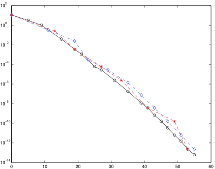
Theorem 3.1 indicates that even if one chooses very close to , the predicted error reduction rate is always bounded from below by the quantity . Such a result looks overly pessimistic, particularly in the case of smooth (analytic) solutions, since a Fourier method allows for an exponential decay of the error as the number of (properly selected) active degrees of freedom is increased. Fig 1 displays the influence of Dörfler parameter on the decay rate and number of solves: choosing closer to 1 does not significantly affect the rate of decay of the error versus the number of activated degrees of freedom, but it significantly reduces the number of iterations. This in turn reduces the computational cost measured in terms of Galerkin solves.
Motivated by this observation, hereafter we consider a variant of Algorithm ADFOUR, which – under the assumptions of Property 2.2 or 2.3 – guarantees an arbitrarily large error reduction per iteration, provided the set of the new degrees of freedom detected by DÖRFLER is suitably enriched.
At the -th iteration, let us define the set by setting
| (3.14) |
where the latter procedure and the value of the integer will be defined later on. We recall that the set is such that satisfies
(see (3.4)). Let be the solution of , which in general will have infinitely many components, and let us split it as
Then, by the minimality property of the Galerkin solution in the energy norm and by (2.5) and (2.9), one has
Thus,
Now we can write ; hence, if is defined in such a way that
then we have
where we have used (2.23). Now, can be chosen to satisfy
| (3.15) |
in such a way that
| (3.16) |
Note that, as desired, the new error reduction rate
| (3.17) |
can be made arbitrarily small by choosing arbitrarily close to . The procedure ENRICH is thus defined as follows:
-
•
Given an integer and a finite set , the output is the set
Note that since the procedure adds a -dimensional ball of radius around each point of , the cardinality of the new set can be estimated as
| (3.18) |
where is the measure of the -dimensional Euclidean unit ball centered at the origin.
It is convenient for future reference to denote by the procedure described in (3.14). We summarize our results in the following theorem.
Theorem 3.3 (contraction property of A-ADFOUR)
Consider the aggressive variant A-ADFOUR of the adaptive algorithm ADFOUR, in which the step is replaced by
where is such that defined in (3.17) is smaller than , and is the smallest integer for which (3.15) is fulfilled. Let the assumptions of Property 2.2 or 2.3 be satisfied. Then, the same conclusions of Theorem 3.1 hold true for this variant, with the contraction factor replaced by .
3.4 C-ADFOUR and PC-ADFOUR: ADFOUR with coarsening
The adaptive algorithm ADFOUR and its variants introduced above are not guaranteed to be optimal in terms of complexity. Indeed, the discussion in the forthcoming Sect. 5 for the exponential case will indicate that the residual may be significantly less sparse than the corresponding Galerkin solution ; in particular, we will see that many indices in , activated in an early stage of the adaptive process, could be lately discarded since the corresponding components of are zero. For these reasons, we propose here a new variant of algorithm ADFOUR, which incorporates a recursive coarsening step.
The algorithm is constructed through the procedures GAL, RES, DÖRFLER already introduced in Sect. 3.1, together with the new procedure COARSE defined as follows:
-
•
Given a function for some finite index set , and an accuracy which is known to satisfy , the output is a set of minimal cardinality such that(3.19)
We will subsequently show (see Theorem 6.1) that the cardinality is optimally related to the sparsity class of . The following result will be used several times in the paper.
Property 3.1 (coarsening)
The procedure COARSE guarantees the bounds
| (3.20) |
and, for the Galerkin solution ,
| (3.21) |
Proof. The first bound is trivial, the second one follows from the minimality property of the Galerkin solution in the energy norm and from (2.5):
Given two parameters and , we define the following adaptive algorithm with coarsening.
Algorithm C-ADFOUR()
-
Set , ,
-
do
-
-
set ,
-
-
do
-
-
while
-
-
-
-
-
while
We observe that the specific choice of accuracy in each call of COARSE in the algorithm above is motivated by the wish of guaranteeing a fixed reduction of the residual and error at each outer iteration. This is made precise in the following theorem.
Theorem 3.4 (contraction property of C-ADFOUR)
The algorithm C-ADFOUR satisfies
-
(i)
The number of iterations of each inner loop is finite and bounded independently of ;
-
(ii)
The sequence of residuals and errors generated for by the algorithm satisfies the inequalities
(3.22) and
(3.23) for
(3.24) In particular, if is chosen in such a way that , for any the algorithm terminates in a finite number of iterations, whereas for the sequence converges to in as .
Proof. (i) For any fixed , each inner iteration behaves as the algorithm ADFOUR considered in Sect. 3.1. Hence, setting again , we have as in Theorem 3.1
which implies, by (2.9),
This shows that the termination criterion
| (3.25) |
is certainly satisfied if
i.e., as soon as
We conclude that the number of inner iterations is bounded by , which is independent of .
(ii) By (2.8), we have
At the exit of the inner loop, the quantity on the right-hand side is precisely the parameter fed to the procedure COARSE; then, Property 3.1 yields
On the other hand, the termination criterion (3.25) yields
so that
This bound together with the left-hand inequality in (2.9) applied to yields (3.22), whereas the same inequality applied to yields (3.23).
A coarsening step can also be inserted in the aggressive algorithm A-ADFOUR considered in Sect. 3.3; indeed, the enrichment step ENRICH could activate a larger number of degrees of freedom than really needed, endangering optimality. The algorithm we now propose can be viewed as a variant of C-ADFOUR, in which the use of E-DÖRFLER instead of DÖRFLER allows one to take a single inner iteration; in this respect, one can consider the enrichment step as a “prediction”, and the coarsening step as a “correction”, of the new set of active degrees of freedom. For this reason, we call this variant the Predictor/Corrector-ADFOUR, or simply PC-ADFOUR.
Given two parameters and , we choose as the smallest integer for which (3.15) is fulfilled, and we define the following adaptive algorithm.
Algorithm PC-ADFOUR()
-
Set , ,
-
do
-
-
while
Theorem 3.5 (contraction property of PC-ADFOUR)
4 Nonlinear approximation in Fourier spaces
4.1 Best -term approximation and rearrangement
Given any nonempty finite index set and the corresponding subspace of dimension , the best approximation of in is the orthogonal projection of upon , i.e. the function , which satisfies
(we set if ). For any integer , we minimize this error over all possible choices of with cardinality , thereby leading to the best -term approximation error
A way to construct a best -term approximation of consists of rearranging the coefficients of in decreasing order of modulus
and setting with . As already mentioned in the Introduction, let us denote from now on the rearranged and rescaled Fourier coefficients of . Then,
Next, given a strictly decreasing function such that for some and when , we introduce the corresponding sparsity class by setting
| (4.1) |
We point out that in applications need not be a (quasi-)norm since need not be a linear space. Note however that always controls the -norm of , since . Observe that iff there exists a constant such that
| (4.2) |
The quantity dictates the minimal number of basis functions needed to approximate with accuracy . In fact, from the relations
and the monotonicity of , we obtain
| (4.3) |
The second addend on the right-hand side can be absorbed by a multiple of the first one, provided is sufficiently small; in other words, it is not restrictive to assume that there exists a constant slightly larger than such that
| (4.4) |
Remark 4.1 (sparsity class for )
Replacing by in (4.1) leads to the definition of a sparsity class, still denoted by , in the space of linear continuous forms on . This observation applies to the subsequent definitions as well (e.g., for the class ). In essence, we will treat in a unified way the nonlinear approximation of a function and of a form .
Throughout the paper, we shall consider two main families of sparsity classes, identified by specific choices of the function depending upon one or more parameters. The first family is related to the best approximation in Besov spaces of periodic functions, thus accounting for a finite-order regularity in ; the corresponding functions exhibit an algebraic decay as , which motivates our terminology of algebraic classes. The second family is related to the best approximation in Gevrey spaces of periodic functions, which are formed by infinitely-differentiable functions in ; the associated ’s exhibit an exponential decay, and for this reason such classes will be referred to as exponential classes. Properties of both families are collected hereafter.
4.2 Algebraic classes
The following is the counterpart for Fourier approximations of by now well-known nonlinear approximation settings [11], e.g. for wavelets or nested finite elements. For this reason, we just state definitions and properties without proofs.
For , let us introduce the function
| (4.5) |
and arbitrary, with inverse
| (4.6) |
and let us consider the corresponding class defined in (4.1).
Definition 4.1 (algebraic class of functions)
We denote by the subset of defined as
It is immediately seen that contains the Sobolev space of periodic functions . On the other hand, it is proven in [12], as a part of a more general result, that for , the Besov space is contained in provided .
Let us associate the quantity to the parameter , via the relation
The condition for a function to belong to some class can be equivalently stated as a condition on the vector of its Fourier coefficients, precisely, on the rate of decay of the non-increasing rearrangement of .
Definition 4.2 (algebraic class of sequences)
Let be the subset of sequences so that
Note that this space is often denoted by in the literature, being an example of Lorentz space.
The relationship between and is stated in the following Proposition.
Proposition 4.1 (equivalence of algebraic classes)
Given a function and the sequence of its Fourier coefficients, one has if and only if , with
At last, we note that the quasi-Minkowski inequality
holds in , yet the constant blows up exponentially as .
4.3 Exponential classes
We first recall the definition of Gevrey spaces of periodic functions in (see [14]). Given reals , and , we set
Note that is contained in all Sobolev spaces of periodic functions , . Furthermore, if , is made of analytic functions.
Gevrey spaces have been introduced to study the and analytical regularity of the solutions of partial differential equations. For our elliptic problem (2.3), the following statement is an example of shift theorem in Gevrey spaces.
Theorem 4.1 (shift theorem)
If the assumptions of Property 2.3 are satisfied, then for any , and , is an isomorphism between and .
Proof. Proceeding as in Sect. 2.3, it is immediate to see that the problem can be equivalently formulated as , where the vectors and contain the Fourier coefficients of functions and normalized in and , respectively. If is a bi-infinite diagonal exponential matrix, then we can write . We observe that property , which implies the thesis, is a consequence of .
To show the latter inequality, we let and notice that
Since , we deduce and , whence
because and the series converges. This implies the desired estimate.
From now on, we fix and we normalize again the Fourier coefficients of a function with respect to the -norm. Thus, we set
| (4.7) |
Functions in can be approximated by the linear orthogonal projection
for which we have
As already observed in Property 2.4, setting , one has , so that
| (4.8) |
Hence, we are led to introduce the function
| (4.9) |
whose inverse is given by
| (4.10) |
and to consider the corresponding class defined in (4.1), which therefore contains .
Definition 4.3 (exponential class of functions)
We denote by the subset of defined as
At this point, we make the subsequent notation easier by introducing the -dependent function
As in the algebraic case, the class can be equivalently characterized in terms of behavior of rearranged sequences of Fourier coefficients.
Definition 4.4 (exponential class of sequences)
Let be the subset of sequences so that
where is the non-increasing rearrangement of .
The relationship between and is stated in the following Proposition.
Proposition 4.2 (equivalence of exponential classes)
Given a function and the sequence of its Fourier coefficients, one has if and only if , with
Proof. Assume first that . Then,
Now, setting for simplicity , one has
The substitution yields
whence . Conversely, let . We have to prove that for any , one has
Let be the largest integer such that (note that ), i.e., . Then,
Now, by Taylor expansion,
so that , and is proven.
Next, we briefly comment on the structure of the set . This is not a vector space, since it may happen that belong to this set, whereas does not. Assume for simplicity that and consider for instance the sequences in
Then,
thus, , so that as , i.e., . On the other hand, we have the following property.
Lemma 4.1 (quasi-triangle inequality)
If for , then with
Proof. We use the characterization given by Proposition 4.2, so that
Given , we seek so that
This implies
and
whence the assertion.
Note that when we obtain thereby extending the previous counterexample.
5 Sparsity classes of the residual
For any finite index set , let be the residual produced by the Galerkin solution . Under Assumption 3.1, the step
selects a set of minimal cardinality in for which . Thus, if belongs to a certain sparsity class , identified by a function , then (4.3) yields
| (5.1) |
Explicitly, if for some , we have by (4.6)
whereas if for some and , we have by (4.10)
We stress the fact that the cardinality of is related to the sparsity class of the residual. We will see in the rest of this section that such a class does coincide with the sparsity class of the solution in the algebraic case, whereas it is different (indeed, worse) in the exponential case. This is a crucial point to be kept in mind in the forthcoming optimality analysis of our algorithms.
The cardinality of depends indeed on how much the sparsity measure deviates from the Hilbert norm . So, before embarking ourselves on the study of the relationship between the sparsity classes of the residual and of the solution, we make some brief comments on the ratio between these two quantities. For shortness, we only consider the exponential case, although similar considerations apply to the algebraic case as well. The size of the ratio
depends on the relative behavior of the rearranged coefficients of , which by Definition 4.4 and Proposition 4.2 satisfy
| (5.2) |
for some constant , with . Let us consider two representative situations.
Example 5.1 (genuinely decaying functions)
The most “favorable” situation is the one in which the sequence of rearranged coefficients decays precisely at the rate given by the right-hand side of (5.2); in other words, suppose that there exists a constant such that for all
| (5.3) |
Then,
and since
we obtain
Thus, if (5.3) is a “tight” bound, the ratio is “small”, and the procedure DÖRFLER activates a moderate number of degrees of freedom at the current iteration.
Example 5.2 (plateaux)
The opposite situation, i.e., the worst scenario, occurs when the sequence of rearranged coefficients of exhibits large “plateaux” consisting of equal (or nearly equal) elements in modulus. Fix an integer arbitrarily large, and suppose that the largest coefficients of satisfy
Since
there exists such that
We conclude that the ratio
turns out to be arbitrarily large, and indeed for such a residual it is easily seen that Dörfler’s condition requires to be of the order of .
Let us now investigate the sparsity classes of the residual, treating the algebraic and exponential cases separately. Note that, in view of Propositions 4.1 or 4.2, for studying the sparsity classes of certain functions and we are entitled to study, equivalently, the sparsity classes of the related vectors and , where is the stiffness matrix (2.10).
5.1 Algebraic case
We first recall the notion of matrix compressibility (see [7] where the concept has been used in the wavelet context).
Definition 5.1 (matrix compressibility)
For , a bounded matrix is called -compressible if for any there exist constants and and a matrix having at most non-zero entries per column, such that
where is summable, and for any , is summable.
Concerning the compressibility of the matrices belonging to the class of Definition 2.1, the following result can be found in [9, Lemma 3.6]. We report here the proof for completeness.
Lemma 5.1 (compressibility)
If , then any matrix is -compressible.
Proof. Let us take , where denotes the integer part plus . Then by Property 2.4 (algebraic case) there holds and has non-vanishing entries per column with . It is immediate to verify that . Moreover, for and setting , we clearly have .
We now consider the continuity properties of the operator between sparsity spaces. The following result is well known (see e.g. [10]) and its proof is here reported for completeness.
Proposition 5.1 (continuity of in )
Let , and . For any , if then , with
The constants appearing in the bounds go to infinity as approaches .
Proof. Let us choose as in the proof of Lemma 5.1. If we set , then by Property 2.4 (algebraic case) we have
On the other hand, for any , let be a best -term approximation of , which therefore satisfies . Note that the difference satisfies as well
Let
where we set . Writing , we obtain
The last equation yields
where the series is convergent but degenerates as approaches . Finally, by construction belongs to a finite dimensional space , where
This implies for any .
At last, we discuss the sparsity class of the residual for some Galerkin solution .
Proposition 5.2 (sparsity class of the residual)
Let the assumptions of Property 2.2 be satisfied, and set . For any , if then for any index set , with
Proof. Denoting by the vector representing and using Proposition 5.1, we get
| (5.4) |
At this point, we invoke the equivalent formulation of the Galerkin problem given by (2.24), which yields . Using and combining Property 2.5 together with Property 2.2, we obtain . Hence, applying Proposition 5.1 to we get
where the last step is an easy consequence of the definition of the projector . By substituting the above inequality into (5.4), we finally obtain
| (5.5) |
where in the last inequality we used again Proposition 5.1.
We observe that the previous bound is tailored to the “worst-scenario”: one expects indeed that for large enough the residual becomes progressively smaller than the solution.
5.2 Exponential case
As already alluded to in the Introduction, and in striking contrast to the previous algebraic case, the implication is false. The following counter-examples prove this fact, and shed light on which could be the correct implication.
Example 5.3 (Banded matrices)
Fix and (hence, ). Recalling the expression (2.14) for the entries of , let us choose , which gives
Next, let us choose for all , which implies (because )
i.e.,
At this point, let us fix a real and an integer , and let us choose the coefficients for to satisfy
In summary, the coefficient of the elliptic operator is a trigonometric polynomial of degree , whereas the coefficient is a constant. The corresponding stiffness matrix is banded with non-zero diagonals, and satisfies
| (5.6) |
In order to define the vector , let us introduce the function , . Let us fix a real and let us define the components of the vector in such a way that
Thus, the rearranged components satisfy , , whence (or, equivalently, ), with , according to Definition 4.4.
The definition of the mapping and the banded structure of imply that the only non-zero components of are those of indices for some and . For these components one has
thus, recalling (5.6), we easily obtain
| (5.7) |
This shows that, for any integer ,
hence
i.e., (or, equivalently, ) regardless of the relative values of and .
On the other hand, let be the smallest integer such that . Given any , let and be such that , which combined with (5.7) yields
The rightmost inequality in (5.7), namely , shows that there are at most components of that are larger than in modulus. This implies , whence
Setting , we conclude that (or, equivalently, ), with
Therefore, the sparsity class of deteriorates from for to with .
Next counter-example shows that, when the stiffness matrix is not banded, in order to have it is not enough to choose some as above, but a choice of is mandatory.
Example 5.4 (Dense matrices)
Let us take again and modify the setting of the previous example, by assuming now that the coefficients satisfy
so that is no longer banded, and its elements satisfy
| (5.8) |
If is an arbitrary integer, we now construct a vector with gaps of size between consecutive non-vanishing entries. To this end, we introduce the function defined as and the vectors with components
From (5.8) and the fact that only the -th entry of does not vanish, we obtain
| (5.9) |
As in Example 5.3, it is obvious that with . However, we will prove below that cannot hold uniformly in for any and .
We start by examining the cardinality of the set
In view of (5.9), the condition is satisfied by those such that
whence and . We now claim that
| (5.10) |
whose proof we postpone. Assuming (5.10) we see that
or equivalently there are about coefficients of with values at least . This implies that the -th rearranged coefficient of satisfies
This proves that for any and , one has
whence the following bound cannot be valid
It remains to prove (5.10). We first note that the sets are disjoint provided . We next set
which is a constant only dependent on . We observe that for every , there holds
| (5.11) |
We write as , make use of (5.9) and the definition of to deduce
Since , the above inequality gives
| (5.12) |
Combining (5.11) and (5.12) yields
By choosing sufficiently large, the last term on the right-hand side of the above inequality can be made arbitrarily small, in particular . We thus get and prove (5.10).
Guided by Examples 5.3 and 5.4, we are ready to state the main result of this section. We define
| (5.13) |
Proposition 5.3 (continuity of in )
Let the differential operator be such that the corresponding stiffness matrix satisfies for some constant . Assume that for some and . Let one of the two following set of conditions be satisfied.
-
(a)
If the matrix is banded with non-zero diagonals, let us set
-
(b)
If the matrix is dense, but the coefficients and satisfy the inequality , let us set
Then, one has , with
| (5.14) |
Proof. We adapt to our situation the technique introduced in [7]. Let () be the differential operator obtained by truncating the Fourier expansion of the coefficients of to the modes satisfying . Equivalently, is the operator whose stiffness matrix is defined in (2.22); thus, by Property 2.4 (exponential case) we have
On the other hand, for any , let be a best -term approximation of (with ), which therefore satisfies , with . Note that the difference consists of a single Fourier mode and satisfies as well
Finally, let us introduce the function defined as , the smallest integer larger than or equal to .
For any , let be the approximation of defined as
Writing , we obtain
We now assume to be in Case (b). Since is continuous, the last equation yields
| (5.15) |
The exponents of the addends can be bounded from below as follows because
with by assumption. Then, (5.15) yields
| (5.16) |
On the other hand, by construction belongs to a finite dimensional space , where
| (5.17) |
This implies
with and as asserted.
We last consider Case (a). One has if , whence if , then the summation in (5.15) can be limited to those satisfying , where . Therefore
Now, if and , whence
We conclude by observing that , since any matrix has at most diagonals.
Finally, we discuss the sparsity class of the residual for any Galerkin solution .
Proposition 5.4 (sparsity class of the residual)
Let and , for constants and according to Property 2.3, and let . If for some and , such that , then there exist suitable positive constants and such that for any index set , with
Proof. We first remark that the hypothesis guarantees (see e.g. [15, Corollary 2.55]); this implies for any , whence the function introduced in (5.13) satisfies for any . Assume for the moment we are given and . By using Proposition 5.3 and Lemma 4.1, we get
| (5.18) |
where, and the following relations hold
From (2.24) we have . Using Property 2.5 and applying Proposition 5.3 to we get
with
By substituting the above inequality into (5.18) and using again Proposition 5.3 we get
| (5.19) |
where
This shows that the thesis holds true for the choice
It remains to verify the assumptions of Proposition 5.3 when is dense. Since and
we have . Moreover, using and yields
which are the required conditions to apply Proposition 5.3 when is dense. This concludes the proof.
Remark 5.1 (definition of )
The limitation stems from the fact that the measure of the unit Euclidean ball in monotonically decreases to as . To avoid such a restriction, one could modify the definition of the Gevrey classes given in (4.7), by replacing the Euclidean norm appearing in the exponential by the maximum norm . Consequently, throughout the rest of the paper would be replaced by the quantity , strictly larger than 1 for any .
6 Coarsening
We start by considering an example that sheds light on the role of coarsening for the exponential case. We then state and prove a seemingly new coarsening result, which is valid for both classes.
6.1 Example of coarsening
Let for be the vectors
Let be the sequences defined by
We first observe that
(recall that for ). Given a parameter , we now construct a perturbation of which is much less sparse than by simply scaling and adding it to (see Fig. 2 (a)):
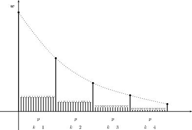
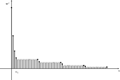
The first task is to compute the norms of . We obviously have . To determine the weak quasi-norm of we need to find the rearrangement (see Fig. 2 (b)). Let be the smallest integer such that
namely the index corresponding to the first crossing of the exponential curve dictating the behavior of the first portion of the rearranged sequence (which coincides with the behavior of ), and the first plateaux of . This implies
Next, let be the smallest integer such that
which corresponds to the beginning of a number of decreasing exponentials preceeding the second plateaux of . This implies
and shows that , and that there is exactly one exponential between the first and second plateaux. Iterating this argument, we see that the difference between two consecutive ’s is just , and that there is exactly one exponential between two consecutive plateaux (see Fig 2 (b)).
We are now ready to compute the weak quasi-norm of . Let denote the index corresponding to the end of the -th plateaux of , which in turn corresponds to the value . Then
To determine the class of , we seek so that , namely
We thus realize that belongs to a sparsity class much worse than that of , that deteriorates as the size of the plateaux tends to . On the other hand, we note that the restrictions coincide, thereby showing that the decay rate of the first part of is the same as that of (see Fig 2(b)). This example explains the need to coarsen the vector starting at latest at , to eliminate the tail of which decays with rate instead of the optimal rate of .
In addition, we observe that the best -term approximation of satisfies
which is precisely the size of the perturbation error of . Given an error tolerance , the best -term approximation of satisfying would require
6.2 New coarsening Result
We extract the following lesson from the example of Sect. 6.1: for as long as we deal with the first part of , which has a decay rate dictated by that of , we could coarsen and obtain an approximation of both and with the decay rate of . This requires limiting the accuracy to size since a smaller accuracy utilizes the tail of which has a slower decay .
We express this heuristics in the following theorem, which goes back to Cohen, Dahmen, and DeVore [7]. However, our proof is much more elementary and the statement much more precise. Although the result holds for the general setting of Sect. 4.1, we just present it for the exponential case, since it will be used only in this situation.
Theorem 6.1 (coarsening)
Let and let and be so that
Let be the smallest integer such that the best -term approximation of satisfies
Then, and
Proof. Let be the set of indices corresponding to the best approximation of with accuracy . So is a minimal set with properties
If , then
because is the projector onto . Since is the cardinality of the smallest set satisfying the above relation, we deduce that . This concludes the proof.
7 Optimality properties of adaptive algorithms: algebraic case
The rest of the paper will be devoted to investigating complexity issues for the sequence of approximations generated by any of the adaptive algorithms presented in Sect. 3. In particular, we wish to estimate the cardinality of each and check whether its growth is “optimal” with respect to the sparsity class of the exact solution, in the sense that is comparable to the cardinality of the index set of the best approximation of yielding the same error .
The algebraic case will be dealt with in the present section, whereas the exponential case will be analyzed in the next one. The two cases differ in that no coarsening is needed for optimality in the former case, whereas we will prove optimality in the latter case only for the algorithms that incorporate a coarsening step. The reason of such a difference can be attributed, on the one hand, to the slower growth of the activated degrees of freedom in the exponential case as opposed to the algebraic case and, on the other hand, to the discrepancy in the sparsity classes of the residuals and the solution in the exponential case, discussed in Sect. 5.2.
7.1 ADFOUR with moderate Dörfler marking
The approach followed in the sequel, which has been proposed in [16] in the wavelet framework and adopted in [21, 6] in the finite-element framework, allows us to prove the optimality of the algorithm in the algebraic case, provided Dörfler marking is not too aggressive.
The two following lemmas will be useful in the subsequent analysis.
Lemma 7.1 (localized a posteriori upper bound)
Let be nonempty subsets of indices. Let and be the Galerkin approximations of Problem (2.4). Then
Proof. One has
because is the support of . The asserted result follows immediately by the Cauchy-Schwarz inequality, upon recalling that for all .
Lemma 7.2 (Dörfler property)
Let be nonempty subsets of indices. Let and be the Galerkin approximations of Problem (2.4). Let the marking parameter satisfies , where , and set . If
for some , then fulfils Dörfer’s condition, i.e.,
Proof. Since in the energy norm because of Pythagoras, the assumption yields
Invoking the lower bound in (3.2) gives
whence applying Lemma 7.1 implies
This concludes the proof.
We are ready to estimate the growth of degrees of freedom generated by the algorithm ADFOUR of Sect. 3.1. For the moment, we place ourselves in the abstract framework of Sect. 4.1, only the final result being specifically for the algebraic case.
Proposition 7.1 (cardinality of )
Proof. Let and make use of (4.4) for : there exists and such that
Let be the overlay of the two index sets, and let be the Galerkin approximation of Problem (2.4). Then, since , we have
Thus, we are entitled to apply Lemma 7.2 to and , yielding
By the minimality property of the cardinality of among all sets satisfying Dörfler property for (Assumption 3.1), we deduce that , i.e.,
| (7.2) |
whence the result.
Corollary 7.1 (cardinality of : general case)
Proof. Recalling that , the previous proposition yields
On the other hand, by Theorem 3.1 one has
| (7.4) |
and we conclude recalling the monotonicity of .
At this point, we assume to be in the algebraic case, i.e. for some . Then, (7.3) reads
Summing-up the geometric series and using (2.5), we arrive at the following result.
Theorem 7.1 (cardinality of : algebraic case)
Under the assumptions of Proposition 7.1, the growth of the active degrees of freedom produced by ADFOUR in the algebraic case is estimated as follows:
where the constant depends only on , and .
This result is “optimal” in that the number of active degrees of freedom is governed, up to a multiplicative constant, by the same law (4.4)-(4.5) as for the best approximation of . The optimality of this result is related to the “sufficiently fast” growth of the active degrees of freedom: the increment of degrees of freedom at each interation may be comparable to the total number of previously activated degrees of freedom (geometric growth).
7.2 A-ADFOUR: Aggressive ADFOUR
We now examine Algorithm A-ADFOUR, defined in Sect. 3.3, which allows the choice of the parameter as close to 1 as desired. Such a feature is in the spirit of high regularity, or equivalently a large value of for . This is a novel approach which combines the contraction property in Theorem 3.3 and the key property of uniform boundedness of the residuals stated in Proposition 5.2.
Theorem 7.2 (cardinality of for A-ADFOUR)
Proof. At each iteration , the set selected by DÖRFLER is minimal, hence by (3.4), (4.3) and (4.6), one has
Using (2.9) and Proposition 5.2, this bound becomes
On the other hand, estimate (3.18) for the procedure ENRICH yields
Now, as in the proof of Corollary 7.1,
| (7.5) |
The contraction property of Theorem 3.3 yields for
with (see 3.17); thus,
Substituting into (7.5), the powers of cancel out, and the asserted estimate follows.
8 Optimality properties of adaptive algorithms: exponential case
From now on, let us assume that for some and . Let us first observe that none of the arguments that led to the complexity estimates of the previous section can be extended to the present situation.
For ADFOUR with moderate Dörfler marking, Corollary 7.1 in which is replaced by its logarithmic expression yields a bound for which is at least times larger than the optimal bound
for the given accuracy (see the proof of Proposition 8.1 for more details, in a similar situation). Manifestedly, the first cause of non-optimality is the crude bound (7.2), which in this case is no longer absorbed by the summation of a geometric series as in the algebraic case.
On the other hand, for A-ADFOUR a sharp estimate of the increment is indeed used in the proof of Theorem 7.2, but this involves the sparsity class of the residual, which in the exponential case may be different from that of the solution, as discussed in Sect. 5.2.
Incorporating a coarsening step in the algorithms allows us to avoid, at least in part, these drawbacks. For these reasons, herafter we investigate the optimality properties of the two algorithms with coarsening presented in Sect. 3
8.1 C-ADFOUR: ADFOUR with coarsening
Let us now discuss the complexity of Algorithm C-ADFOUR, defined in Sect. 3.4. The following optimal result holds.
Theorem 8.1 (cardinality of for C-ADFOUR)
Assume that the solution belongs to , for some and . Then, there exists a constant such that the cardinality of the set of the active degrees of freedom produced by C-ADFOUR satisfies the bound
| (8.1) |
Proof. Since each Galerkin approximation comes just after a call with threshold , Theorem 6.1 yields
On the other hand, (2.5) and Property 3.1 yield
| (8.2) |
Since , this gives the result, up to a shift in the index.
Next, we investigate the optimality of each inner loop. We already know from Theorem 3.4 that the number of inner iterations is bounded independently of . So, we just estimate the growth of degrees of freedom when going from to . We only consider the case of a moderate Dörfler marking, i.e., we subject to the condition stated in Lemma 7.2 (since the case of close to 1 will be covered in the next subsection). The following result holds.
Proposition 8.1 (cardinality of for C-ADFOUR)
Assume that for some and , and that the marking parameter satisfies , where . Then, there exist constants and such that, for all and all , one has
Proof. Each inner loop of C-ADFOUR can be viewed as a truncated version of ADFOUR; hence, the analysis of this algorithm given in Sect. 7.1 can be adapted to the exponential case. In particular, for each increment of degrees of freedom, Proposition 7.1 gives
Since, by (7.4), it follows that
Thus, recalling that by assumption, we have
Combining (3.23), (8.1), and (8.2) with , we conclude the assertion with .
We remark that the previous result provides a complexity bound, relative to the sparsity class of the solution, which is optimal with respect to the index , but suboptimal with respect to the index .
8.2 PC-ADFOUR: Predictor/Corrector ADFOUR
At last, we discuss the optimality of Algorithm PC-ADFOUR, presented in the second part of Sect. 3.4.
Theorem 8.2 (cardinality of PC-ADFOUR)
Suppose that , for some and . Then, there exists a constant such that the cardinality of the set of the active degrees of freedom produced by PC-ADFOUR satisfies the bound
If, in addition, the assumptions of Proposition 5.4 are satisfied, then the cardinality of the intermediate sets activated in the predictor step can be estimated as
where is the input parameter of ENRICH, and , are the parameters which occur in the thesis of Proposition 5.4.
Proof. The proof of the first bound is the same as that of Theorem 8.1. Concerning the second bound, we invoke Proposition 5.4 to write and recall that for each iteration . This, combined with the minimality of the set selected by DÖRFLER, yields
Estimate (3.18) for ENRICH yields
Using (2.8) and Proposition 5.4, this time to replace by and , we obtain the desired result.
We observe that in the case and , the cardinalities and are not bounded by comparable quantities. This looks like a non-optimal result, yet it appears to be intimately related to the fact that in general the residuals belongs to a worse sparsity class than the solution.
Acknowledgements
We wish to thank Dario Bini for providing us with Property
2.3,
and Paolo Tilli for insightful discussions on the exponential classes.
The first and the third author have been partially supported by the Italian research fund PRIN 2008
“Analisi e sviluppo di metodi numerici avanzati per EDP”. The second author has been partially supported by NSF grants DMS-0807811 and DMS-1109325.
References
- [1] P. Binev, A. Cohen, W. Dahmen, R. DeVore, G.P. Petrova, and P. Wojtaszczyk, Congergence rates for greedy algorithms in reduced basis method, SIAM J. Math. Anal. 43 (2011), no. 3, 1457–1472.
- [2] P. Binev, W. Dahmen, and R. DeVore, Adaptive finite element methods with convergence rates, Numer. Math. 97 (2004), no. 2, 219–268.
- [3] D. Bini, Personal communication.
- [4] A. Böttcher and B. Silbermann, Introduction to large truncated Toeplitz matrices, Universitext, Springer-Verlag, New York, 1999.
- [5] C. Canuto, M. Y. Hussaini, A. Quarteroni, and T. A. Zang, Spectral methods, Scientific Computation, Springer-Verlag, Berlin, 2006, Fundamentals in single domains.
- [6] J. M. Cascon, C. Kreuzer, R. H. Nochetto, and K. G. Siebert, Quasi-optimal convergence rate for an adaptive finite element method, SIAM J. Numer. Anal. 46 (2008), no. 5, 2524–2550.
- [7] A. Cohen, W. Dahmen, and R. DeVore, Adaptive wavelet methods for elliptic operator equations – convergence rates, Math. Comp 70 (1998), 27–75.
- [8] A. Cohen, R. DeVore, and R.H. Nochetto, Convergence rates for afem with data, (2011).
- [9] S. Dahlke, M. Fornasier, and K. Groechenig, Optimal adaptive computations in the jaffard algebra and localized frames, Journal of Approximation Theory 162 (201), no. 1, 153 – 185.
- [10] S. Dahlke, M. Fornasier, and T. Raasch, Adaptive frame methods for elliptic operator equations, Adv. Comput. Math. 27 (2007), no. 1, 27–63.
- [11] R. DeVore, Nonlinear approximation, Acta numerica, 1998, Acta Numer., vol. 7, Cambridge Univ. Press, Cambridge, 1998, pp. 51–150.
- [12] R. DeVore and V.N. Temlyakov, Nonlinear approximation by trigonometric sums, J. Fourier Anal. Appl. 2 (1995), no. 1, 29–48.
- [13] W. Dörfler, A convergent adaptive algorithm for Poisson’s equation, SIAM J. Numer. Anal. 33 (1996), no. 3, 1106–1124.
- [14] C. Foias and R. Temam, Gevrey class regularity for the solutions of the Navier-Stokes equations, J. Funct. Anal. 87 (1989), no. 2, 359–369.
- [15] G. B. Folland, Real analysis, second ed., John Wiley & Sons Inc., New York, 1999.
- [16] T. Gantumur, H. Harbrecht, and R. Stevenson, An optimal adaptive wavelet method without coarsening of the iterands, Math. Comp. 76 (2007), no. 258, 615–629.
- [17] S. Jaffard, Propriétés des matrices ”bien localisées” près de leur diagonale et quelques applications, Annales de l’I.H.P. 5 (1990), 461–476.
- [18] P. Morin, R. H. Nochetto, and K. G. Siebert, Data oscillation and convergence of adaptive FEM, SIAM J. Numer. Anal. 38 (2000), no. 2, 466–488 (electronic).
- [19] R. H. Nochetto, K. G. Siebert, and A. Veeser, Theory of adaptive finite element methods: an introduction, Multiscale, nonlinear and adaptive approximation, Springer, Berlin, 2009, pp. 409–542.
- [20] Ch. Schwab, - and -finite element methods, Numerical Mathematics and Scientific Computation, Oxford University Press, New York, 1998.
- [21] R. Stevenson, Optimality of a standard adaptive finite element method, Found. Comput. Math. 7 (2007), no. 2, 245–269.