Quantum criticality in Kondo quantum dot coupled to helical edge states of interacting 2D topological insulators

Abstract

We investigate theoretically the quantum phase transition (QPT) between the one-channel Kondo (1CK) and two-channel Kondo (2CK) fixed points in a quantum dot coupled to helical edge states of interacting 2D topological insulators (2DTI) with Luttinger parameter $0<K<1$. The model has been studied in Ref.TKNg , and was mapped onto an anisotropic two-channel Kondo model via bosonization. For $K<1$, the strong coupling 2CK fixed point was argued to be stable for infinitesimally weak tunnelings between dot and the 2DTI based on a simple scaling dimensional analysisTKNg . We re-examine this model beyond the bare scaling dimension analysis via a 1-loop renormalization group (RG) approach combined with bosonization and re-fermionization techniques near weak-coupling and strong-coupling (2CK) fixed points. We find for $K\rightarrow 1^{-}$ that the 2CK fixed point can be unstable towards the 1CK fixed point and the system may undergo a quantum phase transition between 1CK and 2CK fixed points. The QPT in our model comes as a result of the combined Kondo and the helical Luttinger physics in 2DTI, and it serves as the first example of the 1CK-2CK QPT that is accessible by the controlled RG approach. We extract quantum critical and crossover behaviors from various thermodynamical quantities near the transition. Our results are robust against particle-hole asymmetry for $\frac{1}{2}<K<1$.

I Introduction.

Quantum phase transitions (QPTs)QPT , the continuous phase transitions at zero temperature due to competing quantum ground states or quantum fluctuations, in correlated electron systems are of great fundamental importance and have been intensively studied over the past decades. Very recently, nano-systems (in particular quantum dotsQD ) offer an excellent playground to study QPTs due to high tunabilityhur ; furusaki ; chungDQD ; hofstetter ; affleck ; chung-noneq ; kirchner ; mitra . The well-known Kondo effecthewson ; Kondo plays a crucial role in understanding low energy properties in quantum dot devices. Potential new QPTs in these systems may be realized in connection to exotic Kondo ground states. An outstanding example of an exotic Kondo state is the two-channel Kondo (2CK) system2CK ; Affleck , which has attracted much attention both theoretically and experimentally as it shows non-Fermi liquid behaviors at low temperatures. Experimentally, the 2CK behaviors have been realized in Ref.goldhaber2CK where a quantum dot independently couples to an infinite and a finite reservoirs of non-interacting conduction electrons.

More interestingly, the 2CK physics has also been found theoretically in Kondo quantum dot coupled to two strongly interacting Luttinger liquid leads with Luttinger parameter $K<\frac{1}{2}$gogolin ; kim . In this case, electron-electron interactions in the leads strongly suppress the cross-channel Kondo correlations responsible for charge transport through the quantum dot while the Kondo correlations involving electrons on the same lead are unaffected, leading to an insulating two-channel Kondo ground state where two independent Kondo screenings occur between the spins on the dot and in each lead separately. On the other hand, for weaker electron interactions, $K>\frac{1}{2}$, both kinds of the Kondo scattering involving conduction electrons on the same and different leads become relevant at low energies, giving rise to conducting 1CK ground state where only a single-channel electrons (even combination of the two leads) effectively couple to the Kondo dot. An exotic quantum phase transition between the conducting 1CK phase for $K>\frac{1}{2}$ and the insulating 2CK behaviors for $K<\frac{1}{2}$ is therefore expected at $K=\frac{1}{2}$gogolin . However, the critical properties of this 1CK-2CK QPT have not yet been addressed yet since it is not accessible to any controlled theoretical approaches.

On the other hand, recently a new type of materials–topological insulators (TIs)–with a gaped bulk and gapless edge states has been proposed theoreticallyTIs and realized experimentallyHasan . In 2D TIs, the gapless edge states have “helical” nature, i.e. the directions of spin and momentum are locked togetherSCZhang . Based on bosonization and a simple scaling dimension analysis, the 2CK behaviors were argued to be stabilized in Kondo quantum dot coupled to two interacting helical edge states of 2D TIs as long as a weak electron-electron interaction exists in the helical electrons ($K<1$)TKNg . However, on a general ground, similar competition between the cross-channel Kondo correlation and suppression of tunneling due to electron-electron interactions mentioned above is also expected here for the helical Luttinger liquid, a special type of Luttinger liquid with broken SU(2) symmetry. The exotic 1CK-2CK QPT may therefore occur in this new setup.

In this paper, we re-examine the system in Ref.TKNg near 2CK fixed point to explore the possibility of the exotic 1CK-2CK QPT via the controlled 1-loop renormalization group (RG) approach combined with bosonization, which goes beyond the bare scaling dimension analysis in Ref. TKNg . For a weak but finite lead-dot tunneling, we find that for $K\rightarrow 1^{-}$ the 2CK fixed point can be unstable towards the (anisotropic) 1CK fixed point and the system may undergo a quantum phase transition (QPT) between 1CK and 2CK fixed points. The QPT in our model comes as a result of the combined Kondo and the helical Luttinger physics in 2DTIs. It serves as the first example of the 1CK-2CK QPT that is accessible by the controlled perturbative RG approach. The stability analysis on these two fixed points shows that they are stable against small particle-hole asymmetry for $\frac{1}{2}<K<1$. We extract the non-Fermi liquid behaviors from various thermodynamical quantities at the 1CK-2CK quantum critical point.

This paper is organized as follows. In Sec. II, we introduce the model Hamiltonian and its bosonized form as shown in Ref. TKNg . In Sec. III. A., we present the RG analysis of the model both in the weak coupling limit via bosonization approach (see Appendix A.). In Sec. III. B., we further map our bosonized model onto an effective Kondo model via re-fermionization near the strong-coupling 2CK fixed point. We then perform the RG analysis via both poor-man’s scaling (see Appendix B.) and field-theoretical $\epsilon$-expansion technique (see Appendix C.). Our RG analysis in both limits suggests a quantum phase transition between 1CK and 2CK fixed points. In Sec. IV. we perform stability analysis on the 1CK and 2CK fixed points respectively. We find that both fixed points are stable for $\frac{1}{2}<K<1$, which substantiates our main finding that there exists an unstable quantum critical points separating two stable 1CK and 2CK fixed points near $K=1$. In Sec. V., we calculate via field-theoretical $\epsilon$-expansion approach the critical properties and crossover functions of various thermodynamical observables. In Sec. VI., we emphasize the clear physical picture of our main findings and draw conclusions.

II Model Hamiltonian.

In our set-up, the Kondo Hamiltonian has the same form as in Ref. TKNg , given by:

$$H = H_{0}+H_{K}+H_{int},$$

$$H_{0} = -{\it i}v_{F}\sum_{i=1,2}\int_{-\infty}^{\infty}dx[c^{\dagger\uparrow}_{i,R}(x)\partial_{x}c_{i,R}^{\uparrow}(x)$$

$$- c^{\dagger\downarrow}_{i,L}(x)\partial_{x}c_{i,L}^{\downarrow}(x)],$$

$$H_{K} = \sum_{i=1,2}J_{1}\vec{S}\cdot\vec{s}_{i,i}+\sum_{i\neq j}J_{2}\vec{S}\cdot\vec{s}_{i,j},$$

$$H_{int} = \sum_{i,\sigma=\uparrow\downarrow}g_{4}\int[c^{\dagger\sigma}_{i,\alpha}(x)c_{i,\alpha}^{\sigma}(x)]^{2}dx$$ (1)

$$+ g_{2}\int c^{\dagger\uparrow}_{i,R}(x)c_{i,R}^{\uparrow}(x)c^{\dagger\downarrow}_{i,L}(x)c_{i,L}^{\downarrow}(x)dx.$$

Here, $H_{0}$ describes the two conduction electron baths (labeled as lead $1$ and lead $2$) made of helical edge states in 2D topological insulators, $H_{K}$ is the Kondo interaction, and the electron-electron interactions with forward scattering $g_{2,4}>0$ terms are given by $H_{int}$ with $i=1,2$ the lead index, and $\alpha=R,L$ being the label of the right ($R$) and left ($L$) moving electrons in the helical edge state. The conduction electron spin operator is given by: $\vec{s}_{i,j}=\sum_{k,k^{\prime},\gamma,\delta}c^{\dagger\gamma}_{ki}\cdot\frac{\vec{\sigma}_{\gamma\delta}}{2}\cdot c_{k^{\prime}j}^{\delta}$ with $\gamma,\delta=\uparrow,\downarrow$, $i,j=1,2$. The local impurity spin operator on the quantum dot can be expressed in terms of pseudo-fermion operator $f_{\sigma}$coleman-costi : $\vec{S}=\sum_{\gamma,\delta}f^{\dagger}_{\gamma}\cdot\frac{\vec{\sigma}_{\gamma\delta}}{2}\cdot f_{\delta}$. In the Kondo limit of our interest, the impurity (quantum dot) is singly-occupied: $\sum_{\sigma=\uparrow,\downarrow}f_{\sigma}^{\dagger}f_{\sigma}=1$. Here, the couping $J_{1}$ and $J_{2}$ in $H_{K}$ stand for the strength of the Kondo correlations between the dot and electrons on the same and different leads, respectively. Note that in the presence of spin-orbit coupling, the spins $\uparrow$/$\downarrow$ of the helical edge state electrons are locked with their right-moving ($R$)/left-moving ($L$) momentum. Note also that the small spin-orbit coupling will break the SU(2) spin-rotational symmetry in the above isotropic Kondo model, leading to the anisotropic Kondo model with $J_{i}^{xy}\neq J_{i}^{z}$TKNg .

The Hamiltonian Eq. 1 can be bosonized through the standard Abelian bosonizationbosonization for the electron operatorTKNg ; Kane : $c_{i,R/L}=\frac{1}{\sqrt{2\pi a}}F_{i,R/L}e^{\pm{\it i}(\sqrt{4\pi}\phi_{iR/L}(x)+k_{F}x)}$; the bosonic fields $\phi_{i}(x)=\phi_{iL}(x)+\phi_{iR}(x)$, $\theta_{i}(x)=\phi_{iL}(x)-\phi_{iR}(x)$. The dual fields $\phi_{i}(x)$ and $\theta_{i}(x)$ obey the commutation relations: $[\phi_{i}(x),\theta_{j}(x^{\prime})]=\frac{-{\it i}}{2}\delta_{ij}sgn(x-x^{\prime})$ with $sgn(x=0)=0$. The symmetric and antisymmetric combinations of $\phi_{i}$, $\theta_{i}$ are defined as: $\phi_{s/a}=\frac{1}{\sqrt{2}}(\phi_{1}\pm\phi_{2})$ and $\theta_{s/a}=\frac{1}{\sqrt{2}}(\theta_{1}\pm\theta_{2})$. Here, $F_{i,R/L}$ are the Klein factors to preserve the anti-commutation relations between fermions (electrons) in the bosonsized form, and $a$ is the lattice constant (lower bound in length scale); we have also dropped the spin indices of the edge state electrons due to their helical nature. The bosonized Hamiltonian after rescaling the boson fields is given byTKNg :

$$H = H_{0}+H_{K}$$

$$H_{K} = -a\sqrt{\frac{2\pi}{K}}\frac{J_{1}^{z}}{\pi a}S_{z}\partial_{x}\theta_{s}(0)$$

$$+ \frac{2J_{2}^{z}}{\pi a}S_{z}\sin(\sqrt{\frac{2\pi}{K_{\rho}}}\theta_{a}(0))\sin(\sqrt{\frac{2\pi}{K_{\sigma}}}\phi_{a}(0))$$

$$+ \frac{J_{1}^{xy}}{\pi a}[S^{-}\exp^{-{\it i}(\sqrt{\frac{2\pi}{K_{\sigma}}}\phi_{s}(0))}+h.c.]\cos(\sqrt{\frac{2\pi}{K_{\sigma}}}\phi_{a}(0))$$

$$+ \frac{J_{2}^{xy}}{\pi a}[S^{-}\exp^{-{\it i}(\sqrt{\frac{2\pi}{K_{\sigma}}}\phi_{s}(0))}+h.c.]\cos(\sqrt{\frac{2\pi}{K_{\rho}}}\theta_{a}(0))],$$

$$H_{0} = \frac{v_{F}^{{}^{\prime}}}{2}\int dx(\partial_{x}\phi_{s})^{2}+(\partial_{x}\theta_{s})^{2}+(\partial_{x}\phi_{a})^{2}+(\partial_{x}\theta_{a})^{2}$$

with $K_{\rho}=1/K_{\sigma}=K=\sqrt{\frac{1+\frac{g_{4}}{2}\pi v_{F}-\frac{g_{2}}{2}\pi v_{F}}{1+\frac{g_{4}}{2}\pi v_{F}+\frac{g_{2}}{2}\pi v_{F}}}$ being the Luttinger parameter, $v_{F}^{{}^{\prime}}=v_{F}\sqrt{(1+\frac{g_{4}}{2}\pi v_{F})^{2}-(\frac{g_{2}}{2}\pi v_{F})^{2}}$. Here, we consider repulsive electron-electron interactions ($g_{2},g_{4}>0$), giving $0<K<1$; and $K_{\rho(\sigma)}$ refers to the interaction strength in the charge (spin) sector. Note that $K_{\sigma}=1,K_{\rho}<1$ corresponds to a spinful Luttinger liquid with SU(2) spin symmetry; while as $K_{\sigma}\neq 1$ when this symmetry is broken. The helical Luttinger leads in $H_{0}+H_{int}$ we consider here corresponds to a spinful Luttinger liquid lead with broken SU(2) symmetry and $K_{\sigma}>1$Kane . Note that we have dropped the Klein factors in Eq. LABEL:H_weak_bosonized as they can be included straightforwardly in the same manner as shown in Refs. bosonizedRG ; florens .

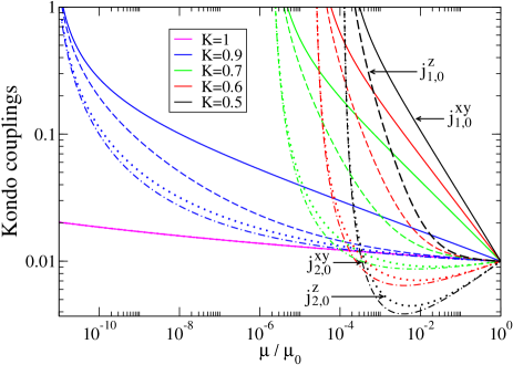
Figure 1: (Color online) RG flows of various Kondo couplings in the weak-coupling regime with fixed bare Kondo couplings: $j_{i,0}^{xy,z}=0.01\mu_{0}$ and $\mu_{0}=1$. Curves with different colors indicate the RG flows with different Luttinger parameters $K$. The solid, dashed, dotted, and dot-dashed lines represent the RG flows for $j_{1}^{xy}$, $j_{1}^{z}$, $j_{2}^{xy}$, and $j_{2}^{z}$, respectively.

III RG analysis of the model.

III.1 RG analysis in weak coupling fixed point: $J_{i}^{xy,z}=0$.

III.1.1 RG scaling equations.

In the vicinity of the fixed point $J_{i}^{xy,z}=0$, it has been shown in Ref. TKNg that the scaling dimensions of these Kondo couplings based on the bosonized Hamiltonian Eq. 1 of Ref. TKNg are: $[J_{1}^{xy}]=K<1,[J_{1}^{z}]=1,[J_{2}^{xy}]=[J_{2}^{z}]=\frac{1}{2}(K+\frac{1}{K})>1$ where $K<1$ for repulsive electron interactions. The authors of Ref. TKNg argued that for $K<1$, under renormalization group (RG) transformations, the 2CK fixed point is reached as the relevant $J_{1}$ couplings flow to large values with decreasing temperatures; while the irrelevant $J_{2}$ couplings decrease to zero. However, for $K$ being slightly less than $1$, $K\rightarrow 1^{-}$, via 1-loop RG, beyond the bare scaling dimension analysis, we find it is possible that all four Kondo couplings can flow to large values, depending on the values of $K$ and the values of the bare Kondo couplings. This seems to suggest the possible existence of the 1CK fixed point in the parameter space of the model.

Following Refs. bosonizedRG ; bosonization via the renormalization group analysis of the bosonized Kondo model Eq. LABEL:H_weak_bosonized, the 1-loop RG scaling equations in the limit of $K\rightarrow 1^{-}$ read (see Appendix A.):

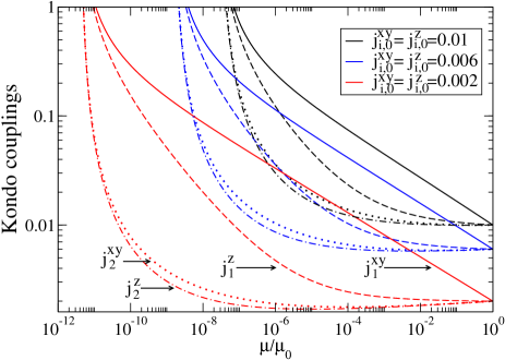
Figure 2: (Color online) RG flows of various Kondo couplings in the weak-coupling regime with fixed $K=0.8$ for various bare Kondo couplings (in units of $\mu_{0}=1$). The solid, dashed, dotted, and dot-dashed lines represent the RG flows for $j_{1}^{xy}$, $j_{1}^{z}$, $j_{2}^{xy}$, and $j_{2}^{z}$, respectively.

$$\frac{\partial j_{1}^{xy}}{\partial\ln\mu} = (K-1)j_{1}^{xy}-j_{1}^{xy}j_{1}^{z}-j_{2}^{xy}j_{2}^{z},$$

$$\frac{\partial j_{1}^{z}}{\partial\ln\mu} = -(j_{2}^{xy})^{2}-(j_{1}^{xy})^{2},$$

$$\frac{\partial j_{2}^{xy}}{\partial\ln\mu} = [\frac{1}{2}(K+\frac{1}{K})-1]j_{2}^{xy}-j_{2}^{xy}j_{1}^{z}-j_{1}^{xy}j_{2}^{z},$$

$$\frac{\partial j_{2}^{z}}{\partial\ln\mu} = [\frac{1}{2}(K+\frac{1}{K})-1]j_{2}^{z}-2j_{1}^{xy}j_{2}^{xy}$$

where $\mu$ is the running cutoff energy scale, and the dimensionless Kondo couplings are defined as: $j_{1}^{xy}\equiv\rho_{0}\mu^{K-1}J_{1}^{xy}$, $j_{1}^{z}=\rho_{0}J_{1}^{z}$, $j_{2}^{xy}=\rho_{0}\mu^{\frac{1}{2}(K+\frac{1}{K})-1}J_{2}^{xy}$, and $j_{2}^{z}=\rho_{0}\mu^{\frac{1}{2}(K+\frac{1}{K})-1}J_{2}^{z}$ with $\mu$ being a cutoff energy scale, and $\rho_{0}=\frac{1}{\pi v_{F}^{\prime}}\equiv\frac{1}{2\mu_{0}}$ being the constant density of states for non-interacting leads ($K=1$) and $\mu_{0}=1$ being the band width of the conduction electrons in the leads. Note that the linear term in the above RG scaling equations comes from the non-trivial scaling dimensions of the corresponding Kondo couplings; while the quadratic terms in Kondo couplings are the corrections at 1-loop order.

For $K\rightarrow 1^{-}$, both $J_{2}^{xy,z}$ terms are marginally irrelevant, $[J_{2}^{xy,z}]\rightarrow 1^{-}$. Therefore, within the validity of perturbative RG, both $J_{2}^{xy,z}$ terms can still flow to a large value if bare Kondo couplings $J_{i}^{xy,z}$ are large enough (but they are still small, $J_{i}^{xy,z}=\mathcal{O}(1-K)\ll 1$) or the electron interactions in the leads are weak enough, leading to (possibly) 1CK fixed point (ie., the quadratic terms overcome the linear term in RG equations). However, for small enough bare Kondo couplings (or strong enough interactions in the leads, $K\ll 1$), $J_{2}^{xy,z}$ terms are irrelevant and hence the system moves towards the 2CK fixed point. As shown in Fig. 1, in the relatively higher temperature (energy) regime $10^{-3}<\mu/\mu_{0}<1$, with decreasing $K$ the system tends to flow to 2CK fixed point where $J_{1}^{xy,z}$ flow to large values while $J_{2}^{xy,z}$ decreases with decreasing temperature (energy). On the other hand, for weak enough interactions in the leads, $K\rightarrow 1^{-}$, all four Kondo couplings tend to flow to 1CK fixed point with large values (see Fig. 1). Similar trend is found for a fixed $K\rightarrow 1$ and different bare Kondo couplings as shown in Fig. 2. It is therefore reasonable to expect a 1CK-2CK quantum phase transition in the parameter space of ${J_{1,2}^{xy,z},K}$. However, the weak coupling RG analysis is valid only at relatively higher energies, and it breaks down as the system gets closer to the ground state, which explains the rapid increase of $J_{2}^{xy,z}$ in Fig. 1 and Fig. 2 at lower temperatures where $J_{1}^{xy}$ already exceeds the perturbative regime, $J_{1}^{xy}>1$. In fact, the low energy behaviors are determined by the physics in the strong coupling regime. Therefore, to address the possible quantum phase transition between 1CK and 2CK fixed points, it is necessary to be able to access the neighborhood of the strong-coupling 2CK fixed point as we shall discuss below.

III.1.2 2-channel Kondo temperature $T_{K}^{2CK}$.

To probe the crossover between 1CK and 2CK fixed points, it is instructive to investigate how the Kondo temperature $T_{K}$ changes with increasing electron-electron interaction in the leads (or with decreasing the value of $K$ from $1$). Since $J_{1}^{xy}$ becomes more relevant with decreasing $K$ in the weak-coupling regime ($[J_{1}^{xy}]=K<1$), it is expected that under RG the system first flows very quickly to the vicinity of 2CK fixed point. As shown in Fig. 3, we find the Kondo temperature $T_{K}^{2CK}$ associated with the 2CK fixed point, defined as the energy scale $\mu=T_{K}^{2CK}$ under RG where $J_{1}^{xy},J_{1}^{z}\approx\mathcal{O}(1)$, increases rapidly with increasing electron interactions in the leads, and its value is much larger than the Kondo temperature of the same setup in the non-interacting limit ($K=1$) $T_{K}^{0}$, $T_{K}^{2CK}\gg T_{K}^{0}$. By contrast, in the case of a Kondo dot coupled to ordinary spinful Luttinger liquid leads in Refs. kim ; gogolin , $J_{1}^{xy}$ is a marginal operator at tree-level ($[J_{1}^{xy}]=1$) in the weak-coupling limit; therefore, the 2CK energy scale $T_{K}^{2CK}$ is much smaller than the Kondo scale for the corresponding non-interacting leads $T_{K}^{0}$, $T_{K}^{2CK}\ll T_{K}^{0}$.

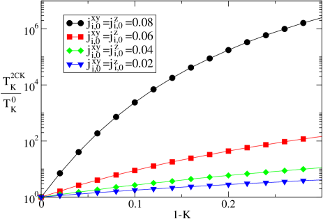
Figure 3: (Color online) The 2CK Kondo temperature $T_{K}^{2CK}$ (in units of $T_{K}^{0}$, the Kondo temperature of the corresponding non-interacting leads, $K=1$) as a function of $1-K$ for various bare Kondo couplings (in units of $\mu_{0}=1$) via the weak-coupling RG analysis.

Though the system in the weak coupling regime quickly approaches the strong-coupling 2CK fixed point as $\mu\rightarrow T_{K}^{2CK}$, the ultimate fate of the ground state depends on the RG flows of various Kondo couplings in the strong coupling regime as discussed below.

III.2 RG analysis near strong coupling (2CK) fixed point.

III.2.1 RG scaling equations and the phase (RG flow) diagram

The authors in Ref. TKNg performed scaling dimension analysis near a strong coupling regime where $J_{1}^{z}=\mathcal{O}(1),J_{2}^{xy,z}=J_{1}^{xy}=0$. They performed the Emery-Kivelson unitary transformationkivelson $U=e^{{\it i}\sqrt{2\pi}\phi_{s}}$ to the bosonized Hamiltonian (Eq. 1 of Ref.TKNg ), and arrived Eq. 2 of Ref. TKNg .

$$H = H_{0}-\tilde{J}_{1}^{z}S_{z}\partial_{x}\theta_{s}(0)$$

$$+ \frac{2J_{2}^{z}}{\pi a}S_{z}\sin(\sqrt{\frac{2\pi}{K}}\theta_{a}(0))\sin(\sqrt{2\pi K}\phi_{a}(0))$$

$$+ (S^{-}+S^{+})[\frac{J_{1}^{xy}}{\pi a}\cos(\sqrt{2\pi K}\phi_{a}(0))$$

$$+ \frac{J_{2}^{xy}}{\pi a}\cos(\sqrt{\frac{2\pi}{K}}\theta_{a}(0))]$$

with $-\tilde{J}_{1}^{z}=\sqrt{2\pi K}v_{F}-\sqrt{\frac{2}{\pi K}}J_{1}^{z}$.

They found the scaling dimensions for the Kondo couplings to be $[J_{1}^{xy}]=\frac{K}{2}$, $[J_{2}^{xy}]=\frac{1}{2K}$, $[J_{2}^{z}]=\frac{1}{2}(K+\frac{1}{K})$. The $J_{1}^{xy}$ term is relevant for $K<1$, and $J_{2}^{xy}$ term is relevant for $\frac{1}{2}<K<1$. As $K\rightarrow 1^{-}$, $J_{2}^{z}$ becomes marginally irrelevant, and it can flow to a large value under RG if the bare Kondo couplings are large enough once the 1-loop RG is performed. This seems to suggest a stable 1CK near strong coupling regime as all of the four Kondo couplings can either flow to or stay at large values (of order $1$).

To gain more insight into the stability of the 1CK/2CK fixed point, we apply RG approach at 1-loop order together with bosonization and re-fermionization near 2CK fixed point. First, we shall map the bosonized Hamiltonian Eq. 1 of Ref. TKNg onto an effective Kondo model via re-fermionization. It has been shown in Ref. TKNg that near the strong coupling 2CK fixed point $J_{1}^{xy}\rightarrow\infty,J_{1}^{z}\rightarrow\mathcal{O}(1),J_{2}^{z/xy}\rightarrow 0$, the effective Hamiltonian reads: $H_{2CK}=H_{0}+\frac{2J_{1}^{xy}}{\pi a}S^{x}\cos(\sqrt{2\pi K}\phi_{a}(0))$. Note that near 2CK fixed point, the dominating “backscattering” $J_{1}^{xy}$ term effectively cuts the Luttinger wire into two separate pieces at $x=0$TKNg ; bosonization , leading to the well-known open boundary condition for an impurity in a Luttinger liquid at $x=0$: $c_{i,R}(0)=-c_{i,L}(0)$ (or $\phi_{iR}(0)=-\phi_{iL}(0)$). The boson field $\phi_{a}$ is approximately pinned to a constant valueTKNg . Also, since $S_{x}$ commutes with $H_{2CK}$, we may therefore set $S_{x}$ to its eigenvalue $\pm\frac{1}{2}$ in $H_{2CK}$. The the scaling dimensions of Kondo couplings near 2CK fixed point areTKNg ; kane-fisher ; bosonization $[J_{2}^{xy}]=\frac{1}{K},[\tilde{J}_{1}^{z}]=1+\frac{1}{2K},[J_{2}^{z}]=\frac{1}{K}+\frac{K}{2}$. Note that all the above three couplings are irrelevant for $K<1$. This suggests that the system favors the 2CK fixed point at ground state $K<1$. Meanwhile, by a stability analysis in Sec. V., we show that the 2CK fixed point is a also a stable fixed point for $K>\frac{1}{2}$ once the system gets there.

However, as suggested in our weak-coupling RG analysis, the 2CK fixed point may be unstable for $K\rightarrow 1^{-}$ and/or large enough bare Kondo couplings such that $J_{2}^{xy,z}$ may become relevant again, and the system can undergo a 1CK-2CK quantum phase transition. To address this possibility, we shall focus below on the 1-loop RG flows of the leading two irrelevant operators near the 2CK fixed point, given by:

$$\delta H_{2CK}=\frac{J_{2}^{xy}}{\pi a}S^{x}\cos(\sqrt{\frac{2\pi}{K}}\theta_{a}(0))-\tilde{J}_{1}^{z}S_{z}\partial_{x}\theta_{s}(0).$$ (5)

Via the similar re-fermionization as shown in Appendix A., we map $H_{0}+\delta H_{2CK}$ onto an effective Kondo model subject to a bosonic environment:

$$H_{0}+\delta H_{2CK} \rightarrow H_{0}+H_{0}^{\prime}+\delta H_{2CK}$$

$$= \tilde{H}_{0}+H_{b}+\tilde{H}_{2CK},$$

$$H_{0}^{\prime} = \frac{v^{{}^{\prime}}_{F}}{2}\int dx(\partial_{x}\theta_{a}^{\prime})^{2}$$

$$\tilde{H}_{0} = \frac{v^{{}^{\prime}}_{F}}{2}\int dx[2(\partial_{x}\theta_{0,a})^{2}+(\partial_{x}\theta_{s})^{2}$$

$$+ (\partial_{x}\phi_{s})^{2}+(\partial_{x}\phi_{a})^{2}]$$

$$= \sum_{k,\sigma,i=1(\tilde{L}),2(\tilde{R})}\epsilon(k)\tilde{c}^{\dagger\sigma}_{k,i}\tilde{c}_{k,i}^{\sigma},$$

$$H_{b} = \frac{v^{{}^{\prime}}_{F}}{2}\int dx2(\partial_{x}\tilde{\theta}_{a})^{2},$$

$$\tilde{H}_{2CK} = J_{2}^{xy}S^{-}[s_{\tilde{L}\tilde{R}}^{+}e^{{\it i}\sqrt{4\pi(\frac{1}{K}-1)}\tilde{\theta}_{a}(0)}$$ (6)

$$+ s_{\tilde{R}\tilde{L}}^{+}e^{-{\it i}\sqrt{4\pi(\frac{1}{K}-1)}\tilde{\theta}_{a}(0)}]+h.c.$$

$$+ \sqrt{\frac{\pi}{2}}\tilde{J}_{1}^{z}(s_{\tilde{L}\tilde{L}}^{z}+s_{\tilde{R}\tilde{R}}^{z})S_{z}$$

where the boson field $\theta_{a}^{\prime}$ in $H_{0}^{\prime}$ is decoupled from $H_{0}$ and is added here just for the mapping, the effective non-interacting electron operator $\tilde{c}_{k,i}^{\sigma}$ is defined in Eq. 9. Note that since the scaling dimension of $\cos(\sqrt{\frac{2\pi}{K}}\theta_{a})$ at 2CK fixed point in Eq. 6 is $\frac{1}{K}$ due to open boundary conditionTKNg , we have made the following decomposition for the boson field $\sqrt{\frac{1}{K}}\theta_{a}$:

$$\sqrt{\frac{1}{K}}\theta_{a} = \sqrt{2}\theta_{0,a}+\sqrt{2}\bar{\theta}_{a},$$

$$\sqrt{\frac{1}{K}}\theta_{a}^{\prime} = \sqrt{2(\frac{1}{K}-1)}\theta_{0,a}-\sqrt{\frac{2}{\frac{1}{K}-1}}\bar{\theta}_{a},$$

$$\theta_{s} = \theta_{0,s},$$

$$\bar{\theta}_{a} = \sqrt{\frac{1}{K}-1}\tilde{\theta}_{a}.$$ (7)

The re-fermionization of $H_{0}$ is done through the following identifications:

$$\sqrt{2}\theta_{0,a} = \sqrt{2}(\phi_{0,1}^{\uparrow}+\phi_{0,2}^{\downarrow})=-\sqrt{2}(\phi_{0,2}^{\uparrow}+\phi_{0,1}^{\downarrow}),$$

$$\sqrt{2}\theta_{0,s} = \phi_{0,1}^{\uparrow}-\phi_{0,1}^{\downarrow}+\phi_{0,2}^{\uparrow}-\phi_{0,2}^{\downarrow}$$

(8)

where we have decomposed the boson field $\sqrt{\frac{1}{K}}\theta_{a}$ into two independent sets of boson fields: the “free” ($\theta_{0,a}$) and “interacting” ($\tilde{\theta}_{a}$) parts: Here, the “free” part of the boson fields $\theta_{0,a}$ (defined in the same way as in Sec.II.) can be re-fermionized into two effective non-interacting fermion leads described by $\tilde{H}_{0}$ with $\tilde{c}_{\alpha}^{\sigma}$ being the electron destruction operator of the effective non-interacting leads

$$\tilde{c}_{i=1(\tilde{L}),2(\tilde{R})}^{\uparrow(\downarrow)}=\frac{1}{\sqrt{2\pi a}}F_{i}^{\uparrow(\downarrow)}e^{\pm{\it i}(\sqrt{4\pi}\phi_{0,i}^{\uparrow(\downarrow)}(x)+k_{F}x)}.$$ (9)

with $\alpha=1(\tilde{L}),2(\tilde{R})$ being the index for effective non-interacting leads, $s_{\gamma\beta}^{\pm(z)}=\sum_{\alpha,\delta,k,k^{\prime}}\frac{1}{2}\tilde{c}_{k\gamma}^{\dagger\alpha}\mathbf{\sigma}_{\alpha\delta}^{\pm(z)}\tilde{c}_{k^{\prime}\beta}^{\delta}$ being the spin-flip (z-component of the spin) operators between the effective leads $\gamma$ and $\beta$. Note that the effective non-interacting leads also exhibit the helical nature; namely, the spin up/down ($\sigma=\uparrow/\downarrow$) electrons are tied to the right (R)/left (L) moving particles, respectively. The “free” part of boson field $\theta_{0,a}$ follow the correlations of the free fremions in 1D:

$$<e^{-{\it i}\sqrt{2\pi}\theta_{0,a}(t)}e^{{\it i}\sqrt{2\pi}\theta_{0,a}(0)}> \propto \frac{1}{t}.$$

Meanwhile, $H_{b}$ represents for the effective dissipative ohmic boson environment (baths) made of the “interacting” part of the effective bosons $\tilde{\theta}_{a}$. These bosons couple to the Kondo dot through the additional exponential “phase” factors in the effective Kondo terms $\tilde{H}_{2CK}$, leading to all the combined Kondo-Luttinger physicsflorens . In particular, since these dissipative ohmic bosons obey the following correlations via Eq. 6:

$$<e^{-{\it i}\sqrt{4\pi(\frac{1}{K}-1)}\tilde{\theta}_{a}(t)}e^{{\it i}\sqrt{4\pi(\frac{1}{K}-1)}\tilde{\theta}_{a}(0)}>\propto\frac{1}{t^{2(\frac{1}{K}-1)}};$$ (11)

while the impurity spin operator $S_{z}$ exhibits the following correlationTKNg :

$$<S_{z}(0)S_{z}(t)>\propto\frac{1}{t^{\frac{1}{K}}}.$$ (12)

These correlations lead to the non-trivial bare scaling dimensions of the Kondo couplings and therefore to the first term (linear in the Kondo coupling) of the RG scaling equations. Note that since near 2CK fixed point $\phi_{s,a}$ fields are decoupled from Eq. 5, we have effectively two independent degrees of freedom left among the four: $(\phi_{s,a},\theta_{s,a})$; the open boundary condition for the spin-up right-moving (R) and spin-down left-moving electrons: $\phi_{0,i}^{\uparrow(R)}=-\phi_{0,i}^{\downarrow(L)}$ is implied in Eq. 8. With the help of Eq. 7 and Eq. 8, , we finally arrive $\tilde{H}_{0}$ and $\tilde{H}_{2CK}$ in Eq. 6.

Next, we shall obtain the one-loop RG scaling equations for $J_{2}^{xy}$ and $\tilde{J}_{1}^{z}$ in Eq.6. To this aim, we define the dimensionless couplings $j_{2}^{xy}\equiv\rho_{0}\tilde{c}_{2}^{\perp}\mu^{\epsilon}J_{2}^{xy}(\mu)$ and $j_{1}^{z}\equiv\rho_{0}\tilde{c}_{1}^{z}\mu^{\epsilon^{\prime}}\tilde{J}_{1}^{z}(\mu)$ and $\epsilon\equiv\frac{1}{K}-1$, $\epsilon^{\prime}\equiv\frac{1}{2K}$ with $\tilde{c}_{1}^{z}$, $\tilde{c}_{2}^{\perp}$ being defined in Appendix B. and C..

We derive the 1-loop RG scaling equations via the poor-man’s scaling approach in Ref. florens (see Appendix B.) and via field-theoretical $\epsilon$-expansion technique (see Appendix C.):

$$\frac{\partial j_{2}^{xy}}{\partial\ln\mu} = \epsilon j_{2}^{xy}-j_{2}^{xy}j_{1}^{z},$$

$$\frac{\partial j_{1}^{z}}{\partial\ln\mu} = \epsilon^{\prime}j_{1}^{z}-(j_{2}^{xy})^{2}.$$ (13)

Figure 4: (Color online) Schematic diagram of the RG flow near 2CK fixed point. The 1CK-2CK quantum critical point (QCP) is represented by the filled black square located at $j_{c}=(j_{1c}^{z},j_{2c}^{xy})=(\epsilon,\sqrt{\epsilon\epsilon^{\prime}})$.

For $K\rightarrow 1^{-}$ we find an intermediate quantum critical fixed point (QCP) at $j_{c}=(j_{1c}^{z},j_{2c}^{xy})=(\epsilon,\sqrt{\epsilon\epsilon^{\prime}})$ within the validity of the perturbative RG separating the 1CK fixed point (for $j_{0}\equiv(j_{1,0}^{z},j_{2,0}^{xy})>j_{c}\equiv(j_{1,c}^{z},j_{2,c}^{xy})$) and 2CK fixed point (for $j_{0}<j_{c}$) where $j_{2}^{xy}$ and $j_{1}^{z}$ flow towards a large and vanishingly small value, respectively (see Fig. 4). The RG flows near the QCP are determined by linearizing the RG scaling equations as shown in Fig. 4. The typical RG flows corresponding to the 1CK and 2CK fixed points are shown in Fig. 5 (a) and (b), respectively.

Note that $j_{1}^{z}\rightarrow 0$ near 2CK fixed point suggests that the original Kondo coupling $J_{1}^{z}$ (see Eq. LABEL:H_K-2CK) is at a large value (order of $1$): $J_{1}^{z}\approx\mathcal{O}(1)$, consistent with the familiar 2CK fixed point with both $J_{1}^{xy,z}$ being large. However, we find the “1CK” fixed point here in the strong-coupling analysis seems somewhat different from the familiar (conventional) 1CK fixed point we obtained in the weak coupling regime where all the four Kondo couplings will flow to (or stay at) large values. Instead, our RG analysis based on re-fermionization for the coupling $j_{2}^{z}=\rho_{0}\tilde{c}_{2}^{z}\mu^{\frac{1}{K}+\frac{2}{K}-1}J_{2}^{z}$ in Eq. LABEL:H_K-2CK near 2CK fixed point shows that it stays irrelevant up to 1-loop order with the RG scaling equation:

$$\frac{\partial j_{2}^{z}}{\partial\ln\mu}=\left[\frac{1}{K}+\frac{K}{2}-1\right]j_{2}^{z}$$ (14)

where we find no corrections at 1-loop order. Note that unlike in the weak coupling RG where $j_{1}^{xy}j_{2}^{xy}$ will contribute to the 1-loop renormalization of $j_{2}^{z}$ (see Eq.LABEL:RGweak, the $j_{1}^{xy}j_{2}^{xy}$ term is absent here in Eq. 14 as $j_{1}^{xy}$ is already very large near the 2CK fixed point, $j_{1}^{xy}(T\approx T_{K}^{2CK})\gg 1$.

Figure 5: (Color online) RG flows of various Kondo couplings in the strong-coupling regime near 2CK fixed point with the following parameters: (a). $j_{i,0}^{xy,z}(\mu=T_{K}^{2CK})=0.4\mu_{0}$, $K=0.8$ and (b). $j_{i,0}^{xy,z}(\mu=T_{K}^{2CK})=0.1\mu_{0}$, $K=0.7$. The RG flows starting from $\mu=T_{K}^{2CK}$ to $\mu\rightarrow 0$ in (a) are towards the 1CK fixed point; while as the flows in (b) are moving towards the 2CK fixed point. The solid, dashed, and dot-dashed lines represent the RG flows for $j_{1}^{z}$, $j_{2}^{xy}$, and $j_{2}^{z}$, respectively. Here, we set $\mu_{0}=1$.

It is clear from Eq. 14 thatTKNg $j_{2}^{xy}(\mu)\propto\mu^{\frac{1}{K}+\frac{K}{2}-1}$, vanishing as $\mu\ll T_{K}^{2CK}$ even for $j_{0}>j_{c}$ where the system eventually flows to the 1CK fixed point (see Fig. 5). By combining the 1-loop RG analysis in the weak and strong coupling limits, we may obtain the full crossover of $J_{2}^{z}$ for the system which will eventually flow to the 1CK fixed point: For $T_{K}^{2CK}<T<\mu_{0}$, $j_{2}^{z}$ first grows to order of $1$ (see Fig.1); then it vanishes in a power-law fashion at lower temperatures $T\ll T_{K}^{2CK}$ (see Fig.5). However, the above qualitative feature for $j_{2}^{z}$ based on the 1-loop RG analysis might get modified at the 2-loop order, which exceeds the scope of our current work and will be addressed elsewhere.

Though somewhat unconventional, the fixed point with $j_{1,2}^{xy},j_{1}^{z}\rightarrow\infty$ and $j_{2}^{z}\rightarrow 0$ can still be regarded as the one-channel Kondo (1CK) fixed point since the two leads are connected by the strong transverse Kondo couplings $j_{2}^{xy}$; and only one channel of conduction electrons (even combination of the two leads) couples to the Kondo dot. Therefore, we expect the linear conductance $G_{\perp}(T)$ contributed from $J_{2}^{xy}$ at the 1CK fixed point here to show the same temperature dependence as those in the isotropic one-channel Kondo system.

III.2.2 1-channel Kondo temperature $T_{K}^{1CK}$

As mentioned above, for $j_{0}>j_{c}$ with decreasing temperature the system crosses over from 2CK to 1CK fixed point at a much lower energy scale $\mu\approx T_{K}^{1CK}\ll T_{K}^{2CK}$ where $T_{K}^{1CK}$ refers to the Kondo temperature associated with the 1CK fixed point. As shown in Fig. 6, the 1CK fixed point persists to be the ground state at a finite but weak electron-electron interaction strength, $K_{c}<K<1$ with $K_{c}$ being the critical interaction below which the ground state switches from 1CK to 2CK fixed point. Meanwhile, the crossover scale to 1CK fixed point $T_{K}^{1CK}$ (with respect to $T_{K}^{2CK}$) for $j_{0}>j_{c}$ gets reduced significantly as interaction gets stronger. Also, for a fixed value of $K$, the ratio $T_{K}^{1CK}/T_{K}^{2CK}$ is larger for larger bare Kondo couplings $j_{0}$, as expected.

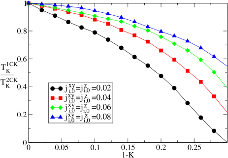
Figure 6: (Color online) The ratio of 1CK to 2CK Kondo temperature $T_{K}^{1CK}/T_{K}^{2CK}$ as a function of $1-K$ for various bare Kondo couplings $j_{i,0}^{xy,z}(\mu=\mu_{0})$ (in units of $\mu_{0}=1$) via the weak-coupling RG analysis.

IV Stability analysis of 1CK and 2CK fixed point for $K<1$.

Having found the possible QPT between 1CK and 2CK fixed points, it is important to perform a stability analysis and study how robust the quantum critical point of our system is against small perturbations. Equivalently, we need to know how stable the 1CK and 2CK fixed points are for $K<1$.

We first examine the stability of the helical Luttinger liquid lead itself. In general there exists the single particle backscattering term due to the interaction of $c_{i,R/L}(0)$ and the quantum dotTKNg : $t^{\prime}c^{\dagger}_{i,R}c_{i,L}+h.c.$. However, this term is forbidden here as it breaks time-reversal symmetry. Meanwhile, for 1-D Hubbard model in general there exists the “spin-flip” backscattering term in $H_{u}$ of the form: $H_{sf}\propto c_{i,L}^{\dagger\uparrow}c_{i,L}^{\downarrow}c_{i,R}^{\dagger\downarrow}c_{i,R}^{\uparrow}+h.c.$. However, due to the helical nature of our leads (or the Right/Left moving electrons are tied to their spins, i.e., only $c_{R(L)}^{\uparrow(\downarrow)}$ electrons exist), this $H_{sf}$ term is therefore absent. Nevertheless, the the Umklapp term that exists on a single bond is allowed by the time-reversal symmetrySCZhang :

$$H_{um} = g_{u}c^{\dagger\uparrow}_{R}(0)c^{\dagger\uparrow}_{R}(0)c_{L}^{\downarrow}(0)$$

$$\times c_{L}^{\downarrow}(0)+h.c.$$

The scaling dimension of this term has been shown to be $[H_{um}]=4K$, suggesting that the helical edge state is unstable towards an insulating phase for $K<\frac{1}{4}$.

We now focus on the effects of the particle-hole (p-h) asymmetry on the stability of these two fixed points as indicated in Refs. gogolin ; florens ; kim that it is the most relevant perturbation for a Kondo dot coupled to Luttinger liquid leads. Let us first address this issue at 2CK fixed point where the two leads are effectively disconnected. The particle-hole asymmetry in our Kondo model generates potential scattering terms of the following formgogolin :

$$H_{1ps} = H_{t}+H_{te},$$

$$H_{t} = t\sum_{k,i,\sigma,\alpha=L,R}c^{\dagger\sigma\alpha}_{k,i}c_{k,i}^{\sigma\alpha},$$

$$H_{t_{e}} = t_{e}\sum_{k,i\neq j\sigma}c^{\dagger\sigma\alpha}_{k,i}c_{k,j}^{\sigma\alpha}+h.c.$$

with $i,j=1(\tilde{L}),2(\tilde{R})$ being the lead index, $\sigma=\uparrow(R),\downarrow(L)$ being spin index, and $R(L)$ being the right (left) moving particles. Here, $t$ and $t_{e}$ terms represent a chemical potential of each lead and a weak tunneling between the disconnected Luttinger leadsKane . Meanwhile, two additional two-particle scattering terms $H_{2p}$ involving tunneling of spin ($t_{\sigma}$) and of charge ($t_{\rho}$) can be generated by the weak tunneling $t_{e}$ via 2nd-order perturbation (see Fig.2 (d) (e) (f) of Ref. Kane ), given by:

$$H_{2ps} = H_{t_{\sigma}}+H_{t_{\rho}},$$

$$H_{t_{\sigma}} = t_{\sigma}\sum_{k}c^{\dagger\uparrow R}_{k,1}c_{k,2}^{\uparrow R}c_{k,2}^{\dagger\downarrow L}c_{k,1}^{\downarrow L}+h.c.$$ (17)

$$H_{t_{\rho}} = t_{\rho}\sum_{k}c_{k,1}^{\dagger\uparrow R}c_{k,2}^{\uparrow R}c_{k,1}^{\dagger\downarrow L}c_{k,2}^{\downarrow L}.$$ (18)

The bosonized form of Eq. LABEL:H2p readsKane :

$$H_{1ps}+H_{2ps} = t\frac{K}{2\pi a}\partial_{x}\phi_{s}$$

$$+ \frac{t_{e}}{2\pi a}\cos(\sqrt{2\pi K}\phi_{a}(0))\cos(\sqrt{\frac{2\pi}{K}}\theta_{a}(0))$$

$$+ \frac{t_{\rho}}{2\pi a}\cos(2\sqrt{2\pi K}\phi_{a})$$

$$+ \frac{t_{\sigma}}{2\pi a}\cos(2\sqrt{\frac{2\pi}{K}}\theta_{a}).$$

Near 2CK, $\phi_{a}(0)$ is a constant, therefore the scaling dimensions of these term gives: $[t]=1$,$[t_{e}]=\frac{1}{2K}$, $[t_{\sigma}]=\frac{2}{K}$ ($t_{\rho}\approx const.$)Kane . It is clear that all operators are irrelevant for $\frac{1}{2}<K<2$; $t_{e}$ term becomes relevant for $K<\frac{1}{2}$, and $t_{\sigma}$ is relevant for $K>2$.

Next, we consider the stability of the 1CK fixed point. Since the cross-channel Kondo coupling $J_{2}^{xy}$ term flows under RG along with $J_{1}^{xy}$ to large values while as $J_{1}^{z}$ stay at order of $1$, the two semi-infinite Luttinger wires are joined into one single infinite Luttinger wireKim. In contrast to the “weak tunneling” processes mentioned above at the 2CK fixed point, the potential scattering term generates the “weak backscattering” processes between the electrons in the upper and lower edges, including the single-particle backscattering term $v_{e}$, and the two-particle backscattering terms $v_{\rho}$, and $v_{\sigma}$ (see Fig. 2 (a) (b) (c) in Ref. Kane ):

$$H_{v_{e}} = v_{e}\sum_{k}c^{\dagger\uparrow R}_{k,1}c_{k,2}^{\uparrow L}+c^{\dagger\downarrow L}_{k,1}c_{k,2}^{\downarrow R}+h.c.,$$

$$H_{v_{\rho}} = v_{\rho}\sum_{k}c_{k,1}^{\dagger\uparrow R}c_{k,2}^{\uparrow L}c_{k,1}^{\dagger\downarrow L}c_{k,2}^{\downarrow R}+h.c.,$$ (21)

$$H_{v_{\sigma}} = v_{\sigma}c^{\dagger\uparrow R}_{k,1}c_{k,2}^{\uparrow L}c_{k,2}^{\dagger\downarrow R}c_{k,1}^{\downarrow L}+h.c.$$ (22)

In fact, there exists a duality mapping between the “weak tunneling” and “weak backscattering” limitsKane : $c_{k,2}^{\uparrow R}\rightarrow c_{k,2}^{\uparrow L},c_{k,2}^{\downarrow L}\rightarrow c_{k,2}^{\downarrow R},t_{e}\rightarrow v_{e},t_{\rho}\rightarrow v_{\sigma},t_{\sigma}\rightarrow t_{\rho},K\rightarrow\frac{1}{K}$. Note that at 1CK fixed point, $\phi_{a}$ is not pinned to a constant as opposed to that in the 2CK case. The scaling dimensions of these terms can be read off straightforwardly: $[v_{e}]=\frac{1}{2}(K+\frac{1}{K})$, $[v_{\rho}]=2K$, and $[v_{\sigma}]=\frac{2}{K}$. The $v_{e}$ term is always irrelevant for $K<1$, while the $v_{\sigma}$ and $v_{\rho}$ terms are irrelevant for $\frac{1}{2}<K<2$ and relevant otherwise.

Based on the above analysis, we find that both 1CK and 2CK fixed point are stable for $\frac{1}{2}<K<1$, and unstable for $K<\frac{1}{2}$. We have checked that our analysis reproduces the well-known results for a Kondo dot coupled to conventional Luttinger liquid leads in Refs. gogolin ; kim ; florens where $[t_{e}]=\frac{1}{2K}$ at 2CK fixed point and $[v_{e}]=\frac{1}{2}(1+K)$ at 1CK fixed point.

As a final remark, we consider here the parity (left-right) symmetric model where $J_{1}=J_{LL}=J_{RR}$ with $J_{LL(RR)}$ being referred to the Kondo couplings involving only the left (right) lead. Nevertheless, parity asymmetry is a relevant perturbation near 2CK fixed point. In the presence of parity asymmetry ($J_{LL}\neq J_{RR}$), the system will flow to the 1CK fixed point with the large bare Kondo couplingsflorens .

V Critical properties near 1CK-2CK quantum phase transition.

The critical properties and crossovers of various thermodynamical quantities near this newly found 1CK-2CK QCP can be obtained via the above RG approach combined with the field-theoretical $\epsilon-$expansion techniqueZinn-Justin ; zarand ; QMSi ; kircan ; lars . We employ here a double-$\epsilon-$expansion with two small expansion parameters $\epsilon$ and $\epsilon^{\prime}$. Our approach is is valid for the Luttinger parameter $K\rightarrow 1^{-}$ as both parameters $\epsilon$ and $\epsilon^{\prime}$ are within perturbative regime: $\epsilon\rightarrow 0$, $\epsilon^{\prime}\rightarrow\frac{1}{2}<1$, and $\epsilon\ll\epsilon^{\prime}$. Following Refs. QMSi ; kircan ; lars , we define the renormalized pseudo-fermion fields $\tilde{f}_{\sigma}$ and the renormalized dimensionless Kondo couplings $j$ as: $f_{\sigma}=\sqrt{Z_{f}}\tilde{f}_{\sigma}$, and $J_{2}^{xy}=\frac{\mu^{-\epsilon}Z_{j^{\perp}}}{\tilde{c}_{2}^{\perp}Z_{f}}j_{2}^{xy}$, $\tilde{J}_{1}^{z}=\frac{\mu^{-\epsilon^{\prime}}Z_{j^{z}}}{\tilde{c}_{1}^{z}Z_{f}}j_{1}^{z}$ with $Z_{f}$ and $Z_{j^{\perp}/z}$ being the renormalization factors for the impurity field and Kondo couplings, respectively and $\mu$ is a renormalization energy scale. The renormalization factors are obtained via minimal subtractions of poleskircan ; QMSi , given by (see Appendix C.):

$$Z_{j^{\perp}} = 1+\frac{j_{1}^{z}}{\epsilon^{\prime}},$$

$$Z_{j^{z}} = 1+\frac{(j_{2}^{xy})^{2}/j_{1}^{z}}{2\epsilon},$$

$$Z_{f} = 1+\frac{(j_{2}^{xy})^{2}}{8\epsilon}+\frac{(j_{1}^{z})^{2}}{16\epsilon^{\prime}}.$$ (24)

Within the field-theoretical RG approach, we have checked that the RG scaling equations in Eq. 13 can be reproduced via calculating the $\beta-$functions: $\beta(j_{i})\equiv\mu\frac{\partial j_{i}}{\partial\mu}|_{j_{i,0}}$ with $\mu$ being an energy scale, $j_{i}=j_{2}^{xy},j_{1}^{z}$ being the renormalized Kondo couplings and $j_{1,0}=j_{1,0}^{z}=J_{1}^{z},j_{2,0}=j_{2,0}^{xy}=J_{2}^{xy}$ being the bare Kondo couplings (see Appendix C.). Below we discuss various critical properties and crossover functions based on field-theoretical $\epsilon$-expansion approach.

V.1 Observables at criticality.

We first calculate various observables at criticality, including correlation length exponent, impurity entropy, dynamical properties of the T-matrix and local spin susceptibility.

V.1.1 Correlation length exponent $\nu$.

The correlation length exponent $\nu$ describes how the correlation length $\xi$ diverges when the system is tuned to the transition: $\xi\propto|t|^{-\nu}$ with $t\equiv\frac{j_{0}-j_{c}}{j_{c}}$ being the dimensionless distance to the QCP. It also gives the power-law vanish of the characteristic crossover energy scale $T^{\ast}$ close to the transition: $T^{*}\propto|t|^{\nu}$. To calculate $\nu$, we first linearize the RG scaling equations Eq.13 near QCP. The correlation length exponent $\nu$ is determined by the largest eigenvalue of the coupled linearized equations, found to be:

$$\nu=\frac{4K}{\sqrt{1+16K\epsilon}-1}=\frac{1}{2\epsilon}+\mathcal{O}(\epsilon^{2},\epsilon^{\prime 2})$$ (25)

where the leading order behavior $\nu\approx\frac{1}{2\epsilon}$ is obtained by expanding the square-root in Eq. 25 in the limit of $\epsilon\ll\epsilon^{\prime}$.

V.1.2 Impurity entropy.

The impurity contribution to the low-temperature entropy near QCP is obtained by a perturbative calculation of the impurity thermodynamic potential $\Omega_{imp}$kircan with respect to the 2CK fixed point and taking the temperature derivative: $S_{imp}=\frac{\partial\Omega_{imp}}{\partial T}$. At QCP and $T=0$ it can be written as:

$$S_{imp}^{QCP}=S_{imp}^{2CK}+\Delta S_{imp}.$$ (26)

where $S_{imp}^{2CK}=\ln\sqrt{2K}=\frac{1}{2}\ln 2K$ is the zero-temperature residual impurity entropy at 2CK fixed point which shows the existence of fractionally degenerate ground stateTKNg ; Affleck ; Fendley , and $\Delta S_{imp}$ is the correction to $S_{imp}^{2CK}$ at QCP. Following similar renormalized perturbative calculations in Ref. kircan , we find

$$\Delta S_{imp}=\pi^{2}\ln 2[\frac{\epsilon(j_{2c}^{xy})^{2}}{4}+\frac{\epsilon^{\prime}(j_{1c}^{z})^{2}}{8}]=\frac{3\epsilon^{2}\pi^{2}\ln 2}{32K}.$$ (27)

Therefore, we have:

$$S_{imp}^{QCP}=\frac{1}{2}\ln 2K+\frac{3\epsilon^{2}\pi^{2}\ln 2}{32K}.$$ (28)

V.1.3 The $T-$matrix.

The conduction electron $T-$matrix, $T_{\alpha\alpha^{\prime}}(\omega)$, in the Kondo model carries important information on the scattering of the conduction electrons from lead $\alpha$ to lead $\alpha^{\prime}$ via the impurity. In particular, $T_{\alpha\alpha^{\prime}}(\omega)$ with $\alpha\neq\alpha^{\prime}$ describes the transport across the dot, detectable in transport measurements. The $T-$matrix is determined from the conduction electron Green functions $G_{\alpha\alpha^{\prime}}(t)=<c_{\alpha}(0)c^{\dagger}_{\alpha^{\prime}}(t)>$ through $G_{\alpha\alpha^{\prime}}=G_{\alpha\alpha^{\prime}}^{0}\delta_{\alpha\alpha^{\prime}}+G_{\alpha\alpha}^{0}(\omega)T_{\alpha\alpha^{\prime}}(\omega)G_{\alpha^{\prime}\alpha^{\prime}}^{0}(\omega)$paaske . Near 2CK fixed point, $T_{\alpha\alpha^{\prime}}(\omega)$ with $\alpha\neq\alpha^{\prime}$ is defined through the propagator, $G_{T}$, of the composite operator $T_{\sigma\alpha}=J_{2}^{xy}e^{{\it i}\sqrt{4\pi(\frac{1}{K}-1)}\tilde{\theta}_{a}(0)}f^{\dagger}_{\sigma}f_{\sigma^{\prime}}\tilde{c}_{\alpha}^{\sigma^{\prime}}$ (see Eq. 6): $T_{\alpha\alpha^{\prime}(\omega)}=G_{T}(\omega)$kircan .

Following the similar calculations in Ref. kircan and Appendix C., we analyze the propagator $G_{T}(\omega)$ near 2CK fixed point and find at zero temperature $Im(T_{\alpha\alpha^{\prime}}^{2CK}(\omega))\propto\frac{1}{\omega^{-\eta_{T}^{2CK}}}$ with the anomalous exponent at the tree level with respect to the 2CK fixed point given by $\eta_{T}^{2CK}=2\epsilon$ (ie., $Im(T_{\alpha\alpha^{\prime}}^{2CK}(\omega))\propto\omega^{2\epsilon}$). Near 1CK-2CK QCP, however, $Im(T_{\alpha\alpha^{\prime}}(\omega))$ acquires an additional anomalous power-law behavior:

$$Im(T_{\alpha\alpha^{\prime}}(\omega))\propto\frac{1}{\omega^{-\eta_{T}^{2CK}-\eta_{T}}}.$$ (29)

where the additional anomalous exponent $\eta_{T}$ is obtained via the renormalization factor $Z_{T}$ for the $T-$matrix propagator $T_{\alpha\alpha^{\prime}}(\omega)$kircan ; QMSi : $\eta_{T}=\beta(j_{2}^{xy})\frac{\partial\ln Z_{T}}{\partial j_{2}^{xy}}|_{j_{2c}^{xy},j_{1c}^{z}}+\beta(j_{1}^{z})\frac{\partial\ln Z_{T}}{\partial j_{1}^{z}}|_{j_{2c}^{xy},j_{1c}^{z}}.$ Here, the renormalization factor $Z_{T}$ is obtained by minimal subtraction of poleskircan ; QMSi : $Z_{T}=\frac{Z_{f}^{2}}{Z_{j^{\perp}}^{2}}$ with $Z_{f}$, $Z_{j^{\perp}}$ given by Eq. 24. We find therefore

$$\eta_{T}=\frac{(J_{2c}^{xy})^{2}}{2}-2j_{1c}^{z}+\frac{(j_{1c}^{z})^{2}}{4}=\frac{\epsilon}{4K}-2\epsilon+\frac{\epsilon^{2}}{4},$$ (30)

and $Im(T_{\alpha\alpha^{\prime}}(\omega))$ at QCP behaves as:

$$Im(T_{\alpha\alpha^{\prime}}(\omega))\propto\omega^{\frac{\epsilon}{4K}+\frac{\epsilon^{2}}{4}}.$$ (31)

V.1.4 Local spin susceptibility $\chi_{zz}(\omega)$.

The local dynamical spin susceptibility $Im(\chi_{zz}(\omega))$ at the impurity (quantum dot) is defined as the time Fourier transform of the spin-spin correlator: $<S_{z}(0)S_{z}(t)>$. At zero temperature, the imaginary part of the local susceptibility, $Im(\chi_{zz}(\omega))$, shows a power-law behavior at QCP:

$$Im(\chi(\omega)_{QCP})\propto\frac{1}{\omega^{-\eta_{\chi}^{2CK}-\eta_{\chi}}}.$$ (32)

Here, $\eta_{\chi}^{2CK}=\epsilon$ is the anomalous exponent of $Im(\chi_{zz}(\omega))$ at the tree level with respect to the 2CK fixed point via the correlator $<S_{z}(0)S_{z}(t)>\propto\frac{1}{t^{\frac{1}{K}}}$ evaluated at 2CK fixed pointTKNg (ie., $Im(\chi_{zz}^{2CK}(\omega))\propto\omega^{\epsilon}$), and $\eta_{\chi}$ is the correction to the anomalous exponent $\eta_{\chi}^{2CK}$ when the system is at QCP. Via $\epsilon-$expansion within the field-theoretical RG frameworkkircan ; QMSi , $\eta_{\chi}$ reads: $\eta_{\chi}=\beta(j_{2}^{xy})\frac{\partial\ln Z_{\chi}}{\partial j_{2}^{xy}}|_{j_{2c}^{xy},j_{1c}^{z}}+\beta(j_{1}^{z})\frac{\partial\ln Z_{\chi}}{\partial j_{1}^{z}}|_{j_{2c}^{xy},j_{1c}^{z}}$ with $Z_{\chi}=Z_{f}^{2}$ being the renormalization factor for the impurity susceptibilitykircan ; QMSi and $Z_{f}$ defined in Eq. 24. Carrying out the above calculations, we arrive at

$$\eta_{\chi}=\frac{(j_{2c}^{xy})^{2}}{2}+\frac{(j_{1c}^{z})^{2}}{4}=\frac{\epsilon}{4K}+\frac{\epsilon^{2}}{4},$$ (33)

and finally $Im(\chi_{zz}^{2CK}(\omega))$ at QCP shows the following power-law behaviors:

$$Im(\chi_{zz}(\omega))\propto\omega^{\epsilon+\frac{\epsilon}{4K}+\frac{\epsilon^{2}}{4}}.$$ (34)

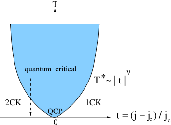
Figure 7: (Color online) Schematic finite temperature phase diagram of our model near 1CK-2CK quantum critical point (QCP) located at $t=0$ ($j_{0}=j_{c}$). As $T\rightarrow 0$, the 1CK ground state is reached when $t>0$ or $j_{0}>j_{c}$; while as the 2CK ground state is reached for $t<0$ or $j_{0}<j_{c}$. Here, $j_{0}>(<)j_{c}$ refers to the upper right (lower left) region in the phase diagram shown in Fig. 4 where the RG flows are towards the 1CK (2CK) fixed point. The dashed vertical arrow at $t<0$ refers to the finite temperature crossover between the quantum critical region (blue shaded area bounded by the crossover temperature $T^{\ast}$) and the 2CK ground state, which is our interest. Here, $j_{0}$ and $j_{c}$ are defined in the text.

V.2 Hyperscaling.

The impurity correlations at QCP is expected to obey certain hyperscaling properties. For example, the local dynamic spin susceptibility at criticality obeys $\frac{\omega}{T}$ scaling in the following form:

$$Im(\chi_{loc}(\omega,T))=\frac{\mathcal{A}}{\omega^{-\eta_{\chi}^{2CK}-\eta_{\chi}}}\Phi(\frac{\omega}{T})$$ (35)

with $\Phi(\frac{\omega}{T})$ being an universal crossover function for the QCP here and $\mathcal{A}$ being a non-universal pre-factor. Similar scaling form can be found in the T-matrix. Hyperscaling can be used to determine relations between various critical exponents. It has been knowningersent ; kircan ; QMSi ; lars that the correlation length exponent $\nu$ and the anomalous exponent $\eta_{\chi}$ are sufficient to determine all critical exponents associated with a local field $h$. In particular, the exponents $\gamma$ and $\gamma^{\prime}$ via the $T\rightarrow 0$ limit of the local susceptibility near criticality are defined asingersent ; lars :

$$\chi_{loc}(t<0;T=0) \propto (-t)^{-\gamma},\;\;\;\gamma=\nu(1-\eta_{\chi}),$$

$$T\chi_{loc}(t>0;T=0) \propto t^{\gamma^{\prime}},\;\;\;\gamma^{\prime}=\nu\eta_{\chi}.$$ (36)

Meanwhile, the critical exponents $\beta$ and $\delta$ associated with the local magnetization $m_{loc}$ can be determined by:

$$m_{loc}(t>0;T=0) \propto t^{\beta},\;\;\;\beta=\frac{1}{2}\nu\eta_{\chi},$$

$$m_{loc}(t=0,T=0) \propto |h|^{\frac{1}{\delta}},\;\;\;\delta=\frac{2}{\eta_{\chi}}-1.$$ (37)

With the values for critical exponents $\nu$ (Eq. 25) and $\eta_{\chi}$ (Eq. 33) at hand, the other critical exponents are therefore given by:

$$\gamma = \frac{1}{2\epsilon}-\frac{1+K\epsilon}{8K}+\mathcal{O}(\epsilon^{2},\epsilon^{\prime 2}),$$

$$\gamma^{\prime} = \frac{1+K\epsilon}{8K}+\mathcal{O}(\epsilon^{2},\epsilon^{\prime 2}),$$

$$\beta = \frac{1+K\epsilon}{16K}+\mathcal{O}(\epsilon^{2},\epsilon^{\prime 2}),$$

$$\delta = \frac{8K}{\epsilon+K\epsilon^{2}}-1+\mathcal{O}(\epsilon^{2},\epsilon^{\prime 2}).$$ (38)

V.3 Crossover near critical point.

Next, we focus on calculating the crossover functions close to the 1CK-2CK quantum critical point. In general, the crossover functions of observables near criticality depend on the RG flows of both $j_{1}^{z}$ and $j_{2}^{xy}$ (see Fig. 7); therefore they may not be expressed analytically in terms of universal crossover functions of a single variable. Nevertheless, great progress can be made when one makes a special choice of bare (initial) values of Kondo couplings such that $\epsilon^{\prime}j_{1,0}^{z}=(j_{2,0}^{xy})^{2}$. Note that this set of bare couplings can in general be tuned through adjusting various microscopic parameters, such as: spin-orbit coupling in 2DTIs, the lead-dot hoping. For this particular choice of bare couplings, we found and checked that the RG flows of $j_{1}^{z}(\mu)$ and $j_{2}^{xy}(\mu)$ follow the well-approximated trajectory: $\epsilon^{\prime}j_{1}^{z}\approx(j_{2}^{xy})^{2}$, (i.e., $\beta(j_{1}^{z})\approx 0$). Under this constraint, only one RG $\beta-$function ($\beta(j_{2}^{xy})$) effectively remains:

$$\beta(j_{2}^{xy})=\epsilon j_{2}^{xy}-2K(j_{2}^{xy})^{3}.$$ (39)

One can therefore easily solve Eq. 39 analytically, and its solution for the range between QCP at $j_{2c}^{xy}=\sqrt{\frac{\epsilon}{2K}}=\sqrt{\epsilon\epsilon^{\prime}}$ and the 2CK fixed point ($j_{2}^{xy}<j_{2c}^{xy}$ where our RG and $\epsilon$-expansion approach is controlled) is found to be:

$$j_{2}^{xy}(\mu)=\frac{j_{2c}^{xy}}{\sqrt{1+(\frac{\mu}{T^{*}})^{-2\epsilon}}}.$$ (40)

where $T^{*}=(\frac{(j_{2c}^{xy})^{2}-(j_{2,0}^{xy})^{2}}{(j_{2,0}^{xy})^{2}})^{\frac{1}{2\epsilon}}$ is the crossover energy scale. It is clear that the power-law vanish of $T^{\ast}$ follows: $T^{\ast}\propto|t|^{\frac{1}{2\epsilon}}\equiv|t|^{\nu}$ with the correlation length exponent $\nu$ being $\nu=\frac{1}{2\epsilon}$, which agrees with our earlier result in Eq. 25. The crossover function in Eq. 40 can be used to compute various crossovers in thermodynamic functions near 1CK-2CK QCP as discussed below.

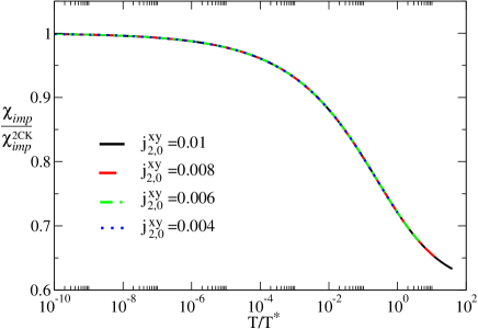
Figure 8: (Color online) $\chi_{imp}/\chi_{imp}^{2CK}$ versus $T/T^{\ast}$ (see Eq.41) at fixed $K=0.8$ for various bare Kondo couplings (in units of $\mu_{0}=1$) where $j_{1}^{z}=2K(j_{2}^{xy})^{2}$ is satisfied and $j_{2c}^{xy}=\sqrt{\frac{\epsilon}{2K}}\approx 0.39$.

V.3.1 The impurity susceptibility $T\chi_{imp}(T)$.

The impurity susceptibility is defined askircan ; lars : $\chi_{imp}(T)=\chi_{imp,imp}+2\chi_{u,imp}+(\chi_{u,u}-\chi^{bulk}_{u,u})$ where $\chi_{u,u}$ is the bulk response to the local field applied to the bulk only, $\chi_{imp,imp}$ is the impurity response to the local filed applied to the impurity only, $\chi_{u,imp}$ is the crossed response of the bulk to an impurity field, $\chi^{bulk}_{u,u}$ is the susceptibility of the bulk in the absence of the impurity. We can calculate $\chi_{imp}(T)$ via perturbative approaches in Refs.kircan ; lars . We find (up to the first order in $j_{2}^{xy}$) $\chi_{imp}(T)$ has the following crossover form (see Eq. 40 and Fig. 8):

$$\frac{\chi_{imp}(T)}{\chi_{imp}^{2CK}(T)} \approx 1-j_{2}^{xy}(\mu\rightarrow T)$$ (41)

$$\approx 1-\frac{j_{2c}^{xy}}{\sqrt{1+(\frac{T}{T^{*}})^{-2\epsilon}}}$$

where $\chi_{imp}^{2CK}$ is the impurity susceptibility at the 2CK fixed point, given bybosonization $\chi_{imp}^{2CK}(T)\propto\frac{\partial C_{imp}^{2CK}}{\partial T}\propto\frac{1}{T^{1-\eta_{\chi_{imp}}^{2CK}}}$ with impurity specific heat at 2CK fixed point given by: $C_{imp}^{2CK}\propto T^{\frac{2}{K}-2}$ (for $\frac{2}{3}<K<1$) and $C_{imp}^{2CK}\propto T$ (for $K<\frac{2}{3}$)TKNg ; gogolin2 . We have therefore $\eta_{\chi_{imp}}^{2CK}=\frac{2}{K}-2$ (for $\frac{2}{3}<K<1$) and $\eta_{\chi_{imp}}^{2CK}=1$ (for $\frac{2}{3}<K<1$).

V.3.2 Impurity entropy $S_{imp}(T)$.

At 2CK fixed point, the impurity residual entropy has been calculated in Ref.TKNg : $S_{imp}^{2CK}=\ln\sqrt{2K}$. Following Ref.kircan , the correction to $S_{imp}^{2CK}$ near QCP is obtained within perturbative RG approach the by calculating the thermodynamic potential and taking the temperature derivative. The crossover function for the impurity entropy near QCP is found to bekircan :

$$\frac{S_{imp}(T)}{S_{imp}^{2CK}} \approx 1+\frac{\pi^{2}\epsilon}{4}\frac{\ln 2}{\ln\sqrt{2K}}[j_{2}^{xy}(\mu\rightarrow T)]^{2}$$ (42)

$$\approx 1+\frac{\pi^{2}\epsilon}{4}\frac{\ln 2}{\ln\sqrt{2K}}[\frac{j_{2c}^{xy}}{\sqrt{1+(\frac{T}{T^{*}})^{-2\epsilon}}}]^{2}.$$

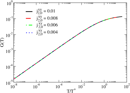
Figure 9: (Color online) Crossover of the linear conductance $G(T)$ versus $T/T^{\ast}$ (see Eq.43) at fixed $K=0.8$ for various bare Kondo couplings (same as in Fig.8).

V.3.3 Equilibrium conductance $G(T)$.

The equilibrium conductance $G(T)$ has the following crossover form between 2CK fixed point and the QCP (see Fig. 9):

$$G(T)\propto[j_{2}^{xy}(\mu\rightarrow T)]^{2}\approx\frac{[j_{2c}^{xy}]^{2}T^{2\epsilon}}{T^{2\epsilon}+(T^{\ast})^{2\epsilon}}.$$ (43)

Note that in equilibrium the linear conductance at 2CK fixed point $G_{2CK}(T)$ is determined by the bare scaling dimension of the leading irrelevant operator $j_{2}^{xy}$, $[j_{2}^{xy}]=\frac{1}{K}$. This gives $G_{2CK}(T)\propto T^{2(\frac{1}{K}-1)}=T^{2\epsilon}$. For $T\ll T^{\ast}$ where the system reaches the 2CK fixed point, the temperature dependence of $G(T)$ in Eq. 43 reduces to that at 2CK, $G(T\ll T^{\ast})\propto G_{2CK}(T)$, as expected.

VI Discussions and Conclusions.

Before we conclude, we would like to emphasize again the clear physical picture we provided in the Introduction to make our main results more transparent. First, it is well-known that the stable one-channel and two-channel Kondo fixed points are expected in the case of Kondo quantum dot coupled to two conventional spinful Luttinger liquid leadsgogolin ; kim . The ground state of this system changes from 1CK to 2CK when Luttinger parameter $K$ reduces from the non-interacting limit ($K=1$) to the strongly interacting limit ($K<\frac{1}{2}$). The electron-electron interactions in the Luttinger liquids act equivalently as if an additional dissipative Ohmic boson bath is coupled to the quantum dothur ; florens , leading to suppression in electron transport from one lead to the other through the dot. A quantum phase transition between 1CK and 2CK fixed points was argued to exist at $K=\frac{1}{2}$ as a direct consequence of the competition between the cross-channel Kondo coupling $J_{LR}$ and the suppression of tunneling due to electron-electron interactiongogolin ; kim . However, up to now there is no analytic and controlled approach to access this transition. Note that the 1-loop RG approach does not work here to reach to the 1CK-2CK quantum critical point since near 2CK fixed point the Kondo couplings $J_{LL/RR}$, involving in the renormalization of the cross-channel Kondo coupling $J_{LR}$, both go to infinity under RG.

When a quantum dot couples to helical Luttinger liquids (a special type of Luttinger liquid), we expect the 1CK and 2CK ground states are also the two possible stable phases for the same reason mentioned above. However, due to the helical nature of the Luttinger liquid leads, the underling two-channel Kondo model becomes anisotropic ($J_{i}^{xy}\neq J_{i}^{z}$) as the $SU(2)$ symmetry of the model is broken; while as the Kondo model is isotropic ($J_{i}^{xy}=J_{i}^{z}$) for a quantum dot coupled to conventional Luttinger liquid leads. This crucial difference enables us to access the QPT between 1CK and 2CK fixed point of our system via the controlled RG approach.

In the limit of a weakly interacting helical liquid $K\rightarrow 1^{-}$, we find the similar competition between these two possible ground states. The 1CK phase is reached when $J_{2}^{xy}$ is large enough; while as the 2CK phase is reached when the electron-electron interaction becomes strong enough. Via a controlled perturbative RG approach at 1-loop order, we find that the 1CK-2CK quantum phase transition occurs near $K=1^{-}$. To reach the 1CK-2CK phase transition in our setup, we believe it is necessary to go beyond the tree-level bare scaling dimension analysis, which predicts a stable 2CK phase for as long as $K<1$TKNg . The 1-loop RG is the leading correction to the above-mentioned bare scaling dimension analysis. Note that the main difference between the case for conventional Luttinger liquid and that for helical liquid is that the resulting two-channel Kondo model is isotropic in the former case; while it is anisotropic in the latter case. This difference affects details of the critical properties, such as: the critical points occurs at $K=K_{c}=\frac{1}{2}$ for the Kondo dot coupled to Luttinger liquid; while as $K_{c}=1-\mathcal{O}(\epsilon)$ for the case of helical Luttinger liquid. At a general level, however, we should expect a 1CK-2CK quantum phase transition to exist in both cases.

In summary, we have re-examined Ref. TKNg on the two-channel Kondo physics in the Kondo quantum dot coupled to two helical edge states of 2-dimensional topological insulators. Via the 1-loop renormalization group approach which goes beyond the scaling dimension analysis in Ref. TKNg , we found the quantum phase transition between the one-channel (1CK) and two-channel (2CK) Kondo ground states for weakly interacting leads ($K\rightarrow 1^{-}$). We made definite predictions on the critical properties when the system is close to the transition. Our results are robust for $\frac{1}{2}<K<1$, and they refine the statement in Ref. TKNg that the two-channel Kondo ground state is stable for as long as $K<1$. Our results also provide the first theoretical realization of the quantum phase transition between 1CK and 2CK physics in Kondo impurity models. Further investigations via field-theoretical and Numerical Renormalization Group (NRG)hewson approaches are needed in order to clarify the critical properties, including the critical exponents and finite-temperature dynamics in crossover functions associated with the transitionlars-florens . Our results could in principle motivate the search for these critical properties near 1CK-2CK quantum phase transition in future experiments on Kondo quantum dot coupled to 2D topological insulators.

Appendix A The RG scaling equation in the weak-coupling regime

In this Appendix, we provide some details on deriving the RG scaling equations of Eq. LABEL:RGweak for $K\rightarrow 1^{-}$ from the bosonized Hamiltonian Eq. LABEL:H_weak_bosonized. Following Refs. bosonizedRG ; bosonization , we decompose the boson fields $\Phi_{\nu}\equiv\theta_{\nu},\phi_{\nu}$ with $\nu=s,a$ into the “fast” ($\Phi_{\nu}^{>}$) and “slow” ($\Phi_{\nu}^{<}$) components:

$$\Phi_{\nu}(\tau) = \Phi_{\nu}^{<}(\tau)+\Phi_{\nu}^{>}(\tau),$$

$$\Phi_{\nu}^{<}(\tau) = \frac{1}{\beta}\sum_{|\omega_{n}|<\mu^{\prime}}\Phi(\omega_{n}),$$

$$\Phi_{\nu}^{>}(\tau) = \frac{1}{\beta}\sum_{\mu^{\prime}<|\omega_{n}|<\mu}\Phi(\omega_{n})$$

with $\mu^{\prime}=\mu+d\mu$. The partition function can be decomposed in the following form:

$$Z_{\mu} = \int D\Phi^{<}D\Phi^{>}e^{-S_{0}[\Phi^{<}]-S_{0}[\Phi^{>}]-S_{int}[\Phi^{>}+\Phi^{<}]},$$

$$= Z_{0}\int D\Phi^{<}e^{-S_{0}[\Phi^{<}]}<e^{-S_{int}[\Phi^{<}+\Phi^{>}]}>_{f}$$

where

$$Z_{0} \equiv \int D\Phi^{>}e^{-S_{0}[\Phi^{>}]},$$

$$<\mathcal{A}>_{f} \equiv \int D\Phi^{>}e^{-S_{0}[\Phi^{>}]}\mathcal{A}[\Phi^{>}].$$ (46)

The partition function $Z_{\mu}$ can be re-expressed by exponentiating $<...>_{f}$ in the integrand in terms of the effective action $S_{eff}[\Phi^{<}]\equiv\int d\tau\mathcal{L}_{K}(\Phi^{<})$ with $\mathcal{L}_{K}$ being the Lagrangian of the Kondo model (see Eq. LABEL:H_weak_bosonized), involving only the slow component of the fields with the following form via the cummulant expansion:

$$S_{eff}[\Phi^{<}] = S_{0}[\Phi^{<}]-\ln<e^{-S_{int}[\Phi^{<}+\Phi^{>}]}>,$$

$$= S_{0}[\Phi^{<}]$$

$$+ <S_{int}[\Phi^{<}+\Phi^{>}]>_{f}$$

$$- \frac{1}{2}(<S_{int}^{2}[\Phi^{<}+\Phi^{>}]$$

$$- <S_{int}[\Phi^{<}+\Phi^{>}]>^{2}_{f}>)+\cdots.$$

The RG procedure is carried out by integrating out the fast modes of bosons and expressing the effective low-energy theory in the original form with the renormalized couplings. The following two-point correlation functions of boson fields prove to be useful in the RG analysisbosonizedRG :

$$G(x,\tau) = <\Phi(x,\tau)\Phi(0,0)>_{f}$$

$$= \int\frac{dk}{2\pi}\int\frac{d\omega}{2\pi}e^{-{\it i}kx}e^{{\it i}\omega\tau}\frac{\pi}{\frac{\omega^{2}}{v_{F}^{\prime}}+v_{F}^{\prime}k^{2}},$$

$$G(\tau) \equiv G(0,\tau)=\left\{\begin{array}[]{ll}\frac{1}{2\pi}K_{0}(\mu^{\prime}\tau)&\mbox{for $\mu^{\prime}\tau>>1$}\\ \frac{1}{2\pi}\ln{\frac{\mu}{\mu^{\prime}}}&\mbox{for $\mu^{\prime}\tau<<1,$}\end{array}\right.$$ (50)

where $K_{0}$ is the Bessel function of the second kind. It is clear from Eq. LABEL:Gtau that $G(\tau)$ can be considered a short-ranged function of $\tau$.

First, we focus on the first order cummulant $<S_{int}[\Phi^{>}+\Phi^{<}]>$, which leads to the bare scaling dimensions of various Kondo couplings in Ref. TKNg . The renormalization of the forward longitudinal term $J_{1}^{z}$ term, $\delta J_{1}^{z}$, gives:

$$J_{1}^{z} \int d\tau<\partial_{x}\theta_{s}(0,\tau)>_{f}$$ (52)

$$= J_{1}^{z}\int d\tau[\partial_{x}\theta_{s}^{<}(0,\tau)+<\partial_{x}\theta_{s}^{>}(0,\tau)>_{f}].$$

Since $\theta_{s}$ is an odd function in spin space, its average vanishes, $<\partial_{x}\theta_{s}^{>}(0,\tau)>_{f}=0$, $\delta J_{1}^{z}=0$. This gives the first-order RG scaling equation:

$$\frac{dj_{1}^{z}}{d\ln\mu}=0$$ (53)

with the renormalized dimensionless coupling $j_{1}^{z}$ defined as: $j_{1}^{z}=\rho_{0}J_{1}^{z}$ where $\rho_{0}=\frac{1}{\pi v_{F}^{\prime}}$ is the density of states. The rescaling of backward longitudinal term $J_{2}^{z}$ term leads to:

$$\int d\tau J_{2}^{z}<\sin(\sqrt{\frac{2\pi}{K}}\theta_{a}(0,\tau))>_{f}<\sin(\sqrt{2\pi K}\phi_{a}(0,\tau))>_{f}$$ (54)

$$= (\frac{\mu^{\prime}}{\mu})^{\frac{K}{2}+\frac{1}{2K}}\times$$

$$\int d\tau J_{2}^{z}\sin(\sqrt{\frac{2\pi}{K}}\theta_{s}^{<}(0,\tau))\sin(\sqrt{2\pi K}\phi_{s}^{<}(0,\tau))$$

where Eq. LABEL:Gtau and $<e^{\mathcal{A}}>=e^{\frac{1}{2}<\mathcal{A}^{2}>}$ are usedbosonization . Upon rescaling $\tau$, $\tau\rightarrow\tau\frac{\mu}{\mu^{\prime}}$, we may define the new dimensionless renormalized coupling $j_{2}^{z}(\mu)$ in terms of the bare coupling $J_{2}^{z}(\mu=\mu_{0}=1)$ as:

$$j_{2}^{z}(\mu)=\rho_{0}\mu^{\frac{K}{2}+\frac{1}{2K}-1}J_{2}^{z},$$ (55)

we arrives at the RG scaling equation at the level of bare scaling dimension:

$$\frac{dj_{2}^{z}}{d\ln\mu}=(\frac{K+1/K}{2}-1)j_{2}^{z}.$$ (56)

The first-order RG scaling equations for the remaining couplings are obtained similarly:

$$\frac{dj_{1}^{xy}}{d\ln\mu} = (K-1)j_{1}^{xy},$$

$$\frac{dj_{2}^{xy}}{d\ln\mu} = (\frac{K+1/K}{2}-1)j_{2}^{xy}$$ (57)

with the renormalized dimensionless couplings defined in the text. Next, we consider the second order cummulant terms generated from $-\frac{1}{2}(<S_{int}^{2}[\Phi^{<}+\Phi^{>}]-<S_{int}[\Phi^{<}+\Phi^{>}]>^{2}>_{f})$. In general, the second-order contributions to the renormalization of various couplings have the following form:

$$\frac{dj_{1}^{xy}}{d\ln\mu} = -a_{1}j_{1}^{xy}j_{1}^{z}-a_{2}j_{2}^{xy}j_{2}^{z},$$

$$\frac{dj_{1}^{z}}{d\ln\mu} = -b_{1}(j_{1}^{xy})^{2}-b_{2}(j_{2}^{xy})^{2},$$

$$\frac{dj_{2}^{xy}}{d\ln\mu} = -c_{1}j_{1}^{xy}j_{2}^{z}-c_{2}j_{2}^{xy}j_{1}^{z},$$

$$\frac{dj_{2}^{z}}{d\ln\mu} = -2d_{1}j_{1}^{xy}j_{2}^{xy},$$

with $a_{i}$, $b_{i}$, $c_{i}$, and $d_{i}$ being the pre-factors to be determined.

We first focus on the terms in $J_{2}^{xy}J_{2}^{z}$ which will contribute to the renormalization of $j_{1}^{xy}$:

$$\frac{2J_{2}^{xy}J_{2}^{z}}{(\pi a)^{2}}S_{z}S^{+}\int d\tau\int d\tau^{\prime}$$

$$\times 2[<e^{-{\it i}\sqrt{2\pi K}\phi_{s}(0,\tau)}\cos(\sqrt{\frac{2\pi}{K}}\theta_{a}(0,\tau))$$

$$\times \sin(\sqrt{\frac{2\pi}{K}}\theta_{a}(0,\tau^{\prime}))\sin(\sqrt{2\pi K}\phi_{a}(0,\tau^{\prime}))>_{f}$$

$$- <e^{-{\it i}\sqrt{2\pi K}\phi_{s}(0,\tau)}\cos(\sqrt{\frac{2\pi}{K}}\theta_{a}(0,\tau))>_{f}$$

$$\times <\sin(\sqrt{\frac{2\pi}{K}}\theta_{a}(0,\tau^{\prime}))\sin(\sqrt{2\pi K}\phi_{a}(0,\tau^{\prime}))>_{f}].$$

After averaging over the fast modes and rescaling $\tau,\tau^{\prime}$, we arrive at:

$$\frac{J_{2}^{xy}J_{2}^{z}}{(\pi a)^{2}}S^{+}\int d\tau\int d\tau^{\prime}(\frac{\mu^{\prime}}{\mu})^{\frac{1}{K}+K-2}$$

$$\times ((\frac{\mu^{\prime}}{\mu})^{\frac{-1}{K}}-1)e^{-{\it i}\sqrt{2\pi K}\phi_{s}^{<}(0,\tau)}\cos(\sqrt{2\pi K}\phi_{a}^{<}(0,\tau^{\prime})),$$

In deriving the above equation, we have decomposed the terms $\sin(\sqrt{2\pi K}(\phi_{a}(\tau^{\prime}))$ and $\cos(\sqrt{\frac{2\pi}{K}}(\theta_{a}(\tau))\sin(\sqrt{\frac{2\pi}{K}}(\theta_{a}(\tau^{\prime}))$ into the fast and the slow modes, and kept only the leading (more relevant) terms. In the limit of $\tau,\tau^{\prime}\ll\frac{1}{\mu}\approx a$, we may get rid off one of the double time-integrals in the above equation by introducing a short-time cutoff $\tau_{0}\approx\frac{a}{v_{F}^{\prime}}$. In the limit of $K\rightarrow 1^{-}$, Eq. LABEL:j2pj2z-bosonized becomes:

$$-\frac{j_{2}^{xy}j_{2}^{z}}{\pi a}S^{+}\int d\tau\frac{d\mu}{\mu}e^{-{\it i}\sqrt{2\pi K}\phi_{s}^{<}(0,\tau)}\cos(\sqrt{2\pi K}\phi_{a}^{<}(0,\tau)).$$ (61)

Therefore, the pre-factor $a_{2}$ in Eq. LABEL:RG-j1j2-bosonized is found to be $a_{2}=1$. Similarly, we find the pre-factors $c_{1}=b_{1}=b_{2}=d_{1}=1$ in Eq. LABEL:RG-j1j2-bosonized.

Next, we consider a different type of renormalization involving $J_{1}^{z}$ terms. We may focus on a typical term $J_{1}^{xy}J_{1}^{z}$, which renormalizes $J_{1}^{xy}$:

$$- a\sqrt{\frac{2\pi}{K}}\frac{J_{1}^{xy}J_{1}^{z}}{(\pi a)^{2}}\int d\tau\int d\tau^{\prime}S^{-}S_{z}$$

$$\times [<\partial_{x}\theta_{s}(0,\tau)$$

$$\times e^{-{\it i}\sqrt{2\pi K}\phi_{s}(0,\tau^{\prime})}\cos(\sqrt{2\pi K}\phi_{a}(0,\tau^{\prime}))>_{f}$$

$$- <\partial_{x}\theta_{s}(0,\tau)>_{f}$$

$$\times <e^{-{\it i}\sqrt{2\pi K}\phi_{s}(0,\tau^{\prime})}\cos(\sqrt{2\pi K}\phi_{a}(0,\tau^{\prime}))>_{f}]$$

$$= -a\sqrt{\frac{2\pi}{K}}\frac{J_{1}^{xy}J_{1}^{z}}{(\pi a)^{2}}\int d\tau\int d\tau^{\prime}S^{-}S_{z}$$

$$\times [<\partial_{x}\theta_{s}^{>}(0,\tau)$$

$$\times e^{-{\it i}\sqrt{2\pi K}\phi_{s}(0,\tau^{\prime})}\cos(\sqrt{2\pi K}\phi_{a}(0,\tau^{\prime}))>_{f}].$$

We may use the following identitiesbosonizedRG to simplify Eq. LABEL:j1pj1z-bosonizedRG:

$$<\partial_{x}\sqrt{\frac{2\pi}{K}}\theta_{s}^{>}(0,\tau)e^{-{\it i}(\sqrt{2\pi K}\phi_{s}(0,\tau^{\prime}))}e^{{\it i}\sqrt{2\pi K}\phi_{a}(0,\tau^{\prime})}>_{f}$$

$$= \lim_{\eta\rightarrow 0}\frac{1}{{\it i}\eta}\partial_{x}<e^{{\it i}\eta\sqrt{\frac{2\pi}{K}}\theta_{a}^{>}(x,\tau)}e^{-{\it i}\sqrt{2\pi K}\phi_{s}^{>}(0,\tau^{\prime})}$$

$$e^{{\it i}\sqrt{2\pi K}\phi_{a}^{>}(0,\tau^{\prime})}>_{f}|_{x=0}$$

$$\times e^{-{\it i}(\sqrt{2\pi K}\phi_{s}^{<}(0,\tau^{\prime}))}e^{{\it i}\sqrt{2\pi K}\phi_{a}^{<}(0,\tau^{\prime})},$$

and

$$e^{\mathcal{A}+\mathcal{B}}=e^{\mathcal{A}}e^{\mathcal{B}}e^{\frac{1}{2}[\mathcal{A},\mathcal{B}]}.$$

(64)

With the above relations, Eq. LABEL:identity1 becomes:

$$\lim_{\eta\rightarrow 0}\frac{1}{{\it i}\eta}\partial_{x}<e^{{\it i}\sqrt{2\pi}(\eta\sqrt{\frac{1}{K}}\theta_{a}^{>}(x,\tau)-\sqrt{K}\phi_{s}^{>}(0,\tau^{\prime}))}>_{f}|_{x=0}$$

$$\times <e^{{\it i}\sqrt{2\pi K}\phi_{a}^{>}(0,\tau^{\prime})}>_{f}$$

$$\times e^{-{\it i}\sqrt{2\pi K}\phi_{s}^{<}(0,\tau^{\prime})}e^{{\it i}\sqrt{2\pi K}\phi_{a}^{<}(0,\tau^{\prime})},$$

$$= \frac{1}{{\it i}}(\frac{\pi}{K}\partial_{x}G_{\theta^{>}_{s}(x,\tau)}+2\pi\partial_{x}<\theta^{>}_{s}(x,\tau)\phi_{s}^{>}(0,\tau^{\prime})>_{f})|_{x=0}$$

$$\times <e^{{\it i}\sqrt{2\pi K}\phi_{s}^{>}(0,\tau^{\prime})}>_{f}<e^{{\it i}\sqrt{2\pi K}\phi_{a}^{>}(0,\tau^{\prime})}>_{f}$$

The leading logarithmic correction comes from the term $\partial_{x}<\theta_{s}^{>}(x,\tau)\phi_{s}^{>}(0,\tau^{\prime})>_{f}$, which can be evaluated via the following relationsbosonizedRG :

$$- \frac{{\it i}}{v_{F}^{\prime}}\frac{\partial\phi_{s}}{\partial\tau}=\frac{\partial\theta_{s}}{\partial x},$$

$$- \frac{{\it i}}{v_{F}^{\prime}}\frac{\partial\theta_{s}}{\partial\tau}=\frac{\partial\phi_{s}}{\partial x}.$$

We have therefore

$$\partial_{x}<\theta_{s}^{>}(x,\tau)\phi_{s}^{>}(0,\tau^{\prime})>_{f} = \frac{-{\it i}}{v_{F}^{\prime}}\frac{\partial}{\partial\tau}<\theta_{s}^{>}(x,\tau)\theta_{s}^{>}(0,\tau^{\prime})>_{f}.$$

After collecting all the terms and performing re-scaling, Eq. LABEL:j1pj1z-bosonizedRG becomes:

$$-\frac{1}{\pi v_{F}^{\prime}}\frac{J_{1}^{xy}J_{1}^{z}}{\pi a}\int d\tau S^{-}(\frac{\mu^{\prime}}{\mu})^{K-1}\frac{d\mu}{\mu}$$

$$\times e^{-{\it i}(\sqrt{2\pi K}\phi_{s}^{<}(0,\tau^{\prime}))}\cos(\sqrt{2\pi K}\phi_{a}^{<}(0,\tau^{\prime})).$$

Finally, the correction to $j_{1}^{xy}$ contributed from $J_{1}^{xy}J_{1}^{z}$, $\delta j_{1,j_{1}^{xy}j_{1}^{z}}^{xy}$, reads:

$$\delta j_{1,j_{1}^{xy}j_{1}^{z}}^{xy} = -j_{1}^{xy}j_{1}^{z}\frac{d\mu}{\mu}\int d\tau e^{-{\it i}\sqrt{2\pi K}\phi_{s}^{<}(0,\tau)}$$ (69)

$$\times \cos(\sqrt{2\pi K}\phi_{a}^{<}(0,\tau)).$$

We therefore find $a_{1}=1$. Similarly, we find $c_{2}=1$. Combining the first and second order corrections to the renormalization of various Kondo couplings, Eq. LABEL:RGweak follows.

Appendix B The 1-loop RG scaling equations near 2CK fixed point via poor-man’s scaling.

In this Appendix, we derive the RG equations in Eq. 13 from the effective Kondo Hamiltonian Eq. 6 in the weak coupling regime via poor-man’s scaling as shown in Ref. florens . Based on the scaling dimensions of various Kondo couplings in the strong couping 2CK regime, we take the logarithmic derivative of the proposed new dimensionless Kondo couplings $j_{2}^{xy}\equiv\rho_{0}\tilde{c}_{2}^{\perp}\mu^{\epsilon}J_{2}^{xy},j_{1}^{z}\equiv\rho_{0}\tilde{c}_{1}^{z}\mu^{\epsilon^{\prime}}\tilde{J}_{1}^{z}$ (see text) with respect to the cutoff energy $\mu$.

First, we focus on the RG equation for $j_{2}^{xy}$:

$$\frac{\partial j_{2}^{xy}}{\partial\ln\mu}=\epsilon j_{2}^{xy}-\mu^{\epsilon}\rho_{0}\tilde{c}_{2}^{\perp}\frac{\partial J_{2}^{xy}}{\partial\ln\mu}.$$ (70)

The derivative of $J_{2}^{xy}$ w.r.t. $\ln\mu$ is given by:

$$\frac{\partial J_{2}^{xy}}{\partial\ln\mu}=\frac{\partial}{\ln\mu}\int_{\mu_{0}}^{\mu}d\omega[J_{2}^{xy}\tilde{J}_{1}^{z}\frac{\rho_{2xy,1z}(\omega)}{-\omega}].$$ (71)

Here, $\rho_{2xy,1z}(\omega)$ is the effective electron density of states due to the additional phase correlations associated with the product of $J_{2}^{xy}$ and $\tilde{J}_{1}^{z}$ terms in Eq. 6. Following Ref. florens , this is equivalent to replacing the free electron Green’s function of the effective leads: $G_{\alpha,0}^{\sigma}(t)\equiv<\tilde{c}^{\dagger\sigma}_{\alpha}(t)\tilde{c}_{\alpha}^{\sigma}(0)>$ by a “mixed” one:

$$\tilde{G}_{\tilde{L}}^{\uparrow(\downarrow)}(t) \equiv <\tilde{c}^{\dagger\uparrow(\downarrow)}_{\tilde{L}}(t)\tilde{c}_{\tilde{L}}^{\uparrow\downarrow}(0)$$

$$\times e^{\pm{\it i}\sqrt{4\pi(\frac{1}{K}-1)}\tilde{\theta}_{a}(t)}S^{\pm}(0)S_{z}(t)>$$

$$\approx G_{\tilde{L},0}^{\uparrow(\downarrow)}(t)$$

$$\times <e^{\pm{\it i}\sqrt{4\pi(\frac{1}{K}-1)}\tilde{\theta}_{a}(t)}><S^{\pm}(0)S_{z}(t)>.$$

($\tilde{G}_{\tilde{R}}^{\sigma}(t)$ can be defined similarly.)

Therefore, $\rho_{2xy,1z}(\omega)\equiv\frac{-1}{\pi}\sum_{\sigma}Im(\tilde{G}_{\alpha}^{\sigma}(\omega))$ readsflorens :

$$\rho_{2xy,1z}(\omega) = \rho_{0}\int_{0}^{\omega}dEP_{2\perp 1z}(E),$$

$$P_{2\perp 1z}(E) = \frac{1}{2\pi}\int dt<\hat{O}_{2\perp 1z}(t)>e^{{\it i}Et}$$ (73)

where $\rho_{0}=\frac{-1}{\pi}\sum_{\sigma}Im(G_{\alpha,0}^{\sigma}(\omega))$ is the constant density of states of the non-interacting leads, and $<\hat{O}_{2\perp 1z}(t)>$ has the following typical form:

$$<\hat{O}_{2\perp 1z}(t)>=<e^{\pm{\it i}\sqrt{4\pi(\frac{1}{K}-1)}\tilde{\theta}_{a}(t)}><S^{\pm}(0)S_{z}(t)>.$$ (74)

Since the exponential factors in $\hat{O}_{2\perp 1z}(t)$ are un-paired, it gives a trivial result: $<e^{\pm{\it i}\sqrt{4\pi(\frac{1}{K}-1)}\tilde{\theta}_{a}(t)}>=1$, and hence it does not affect the renormalization of the couplingsflorens . Nevertheless, $<S^{\pm}(0)S_{z}(t)>$ shows non-trivial correlations nearTKNg :

$$<S^{\pm}(0)S_{z}(t)>\approx\frac{1}{({\it i}\omega_{c}t)^{\epsilon^{\prime}}}$$ (75)

with $\omega_{c}$ being a high-energy cutoff. We have therefore

$$\rho_{2xy,1z}(\omega) = \rho_{0}\int_{0}^{\omega}dEP_{2\perp 1z}(E)=\rho_{0}\tilde{c}_{2}\omega^{2\epsilon^{\prime}},$$

$$P_{2\perp 1z}(E) = \frac{1}{2\pi}\int dt<\hat{O}_{2\perp 1z}(t)>e^{{\it i}Et}=\tilde{c}_{2}^{\perp}E^{\epsilon^{\prime}-1}$$

with $\tilde{c}_{2}=A(\epsilon^{\prime})=\frac{1}{\pi\omega_{c}^{\epsilon^{\prime}}}\sin(\pi\epsilon^{\prime})\Gamma(1+\epsilon^{\prime})$ with $\epsilon^{\prime}=\frac{1}{2K}$ and $\Gamma$ being the Gamma function.

The integral in Eq. 71 gives:

$$\rho_{0}^{2}\tilde{c}_{2}^{\perp}\mu^{\epsilon}J_{2}^{xy}J_{1}^{z}\int_{\mu_{0}}^{\mu}d\omega\frac{\rho_{2xy,1z}(\omega)}{-\omega}$$ (77)

$$= -\rho_{0}^{2}\tilde{c}_{2}^{\perp}A(\epsilon^{\prime})\mu^{\epsilon}\mu^{\epsilon^{\prime}}J_{2}^{xy}J_{1}^{z}\ln\frac{\mu}{\mu_{0}}.$$

Similarly, we find the RG scaling equation for $j_{1}^{z}$ is given by:

$$\frac{\partial j_{1}^{z}}{\partial\ln\mu} = \epsilon^{\prime}j_{1}^{z}-\rho_{0}^{2}\tilde{c}_{1}^{z}A(2\epsilon)\mu^{2\epsilon}(J_{2}^{xy})^{2}$$

where the effective density of states is usedflorens :

$$\rho_{2\perp,2\perp}(\omega) = \rho_{0}\int_{0}^{\omega}dEP_{2\perp 2\perp}(E),$$

$$P_{2\perp 2\perp}(E) = \int dt<\hat{A}(t)>e^{{\it i}Et},$$

$$<\hat{A}(t)> = <e^{-{\it i}\sqrt{4\pi(\frac{1}{K}-1))}\tilde{\theta}_{a}(t)}e^{{\it i}\sqrt{4\pi(\frac{1}{K}-1)}\tilde{\theta}_{a}(0)}>$$

$$\approx \frac{1}{({\it i}\omega_{c}t)^{2\epsilon}}.$$

We may determine the pre-factors $\tilde{c}_{2}^{\perp},\tilde{c}^{z}$ by the following identifications: $\tilde{c}_{2}^{\perp}=\sqrt{A(\epsilon)A(\epsilon^{\prime})}$, $\tilde{c}_{1}^{z}=A(\epsilon^{\prime})$. With the above results, we finally arrive at RG scaling equations shown in Eq.13.

Appendix C The 1-loop RG equations near 2CK fixed point via $\epsilon$-expansion technique.

In this Appendix, we offer an alternative route to Eq. 13 via $\epsilon$-expansion techniqueZinn-Justin ; zarand ; QMSi ; kircan ; lars .

We first derive the renormalization factors $Z_{j^{\perp/z}}$ and $Z_{f}$ shown in Eq. 24. We focus on the 1-loop renormalization of the dimensionless bar couplings $\tilde{j}_{2}^{xy}\equiv\rho_{0}\tilde{c}_{2}^{\perp}\mu^{\epsilon}J_{2}^{xy}$, and $\tilde{j}_{1}^{z}\equiv\rho_{0}\tilde{c}_{1}^{z}\mu^{\epsilon^{\prime}}J_{1}^{z}$. Let us look at vertex renormalization of $j_{1}^{z}$ firstQMSi ; kircan :

$$j_{1}^{z} \equiv Z^{-1}_{j^{z}}\tilde{j}_{1}^{z}=\tilde{j}_{1}^{z}[1+\frac{(J_{2}^{xy})^{2}}{\tilde{j}_{1}^{z}}\int^{\mu}d\omega\frac{\rho_{\perp}(\omega)}{-\omega}]$$ (80)

where the effective density of states readsflorens :

$$\rho_{\perp}(\omega) = \rho_{0}\int_{0}^{\omega}dEP_{\perp}(E),$$

$$P_{\perp}(E) = \int dt<\hat{A}(t)>e^{{\it i}Et},$$

$$<\hat{A}(t)> = <e^{-{\it i}\sqrt{4\pi}\tilde{\theta}_{a}(t)}e^{{\it i}\sqrt{4\pi}\tilde{\theta}_{a}(0)}>\approx\frac{1}{({\it i}\omega_{c}t)^{2\epsilon}}.$$

From above, we find $P_{\perp}(E)=\tilde{c}_{1}E^{2\epsilon-1}$ with $\tilde{c}_{1}=A(2\epsilon)$ and the constant $A(\epsilon)$ being defined in Appendix B..

Therefore, we have

$$\rho_{\perp}(\omega)=\rho_{0}\tilde{c}_{1}\omega^{2\epsilon}.$$ (82)

Plugging in these results into Eq. 80 and via the proper identification: $\tilde{c}_{2}^{\perp}\equiv\sqrt{\tilde{c}_{1}}=\sqrt{A(2\epsilon)}$, at the leading order in $(j_{2}^{xy})^{2}/j_{1}^{z}$, $Z_{j^{z}}$ reads:

$$Z_{j^{z}}=1+\frac{(j_{2}^{xy})^{2}/j_{1}^{z}}{2\epsilon}.$$ (83)

Similarly, we can show that

$$Z_{j^{\perp}}=1+\frac{j_{1}^{z}}{\epsilon^{\prime}}$$ (84)

where the following relations are used:

$$\rho_{z}(\omega) = \frac{\rho_{0}}{2\pi}\int_{0}^{\omega}dEP_{z}(E)=\rho_{0}\tilde{c}_{2}\omega^{2\epsilon^{\prime}},$$

$$P_{z}(E) = \int dt<\hat{B}(t)>e^{{\it i}Et}=\tilde{c}_{2}E^{\epsilon^{\prime}-1},$$

$$\hat{B}(t) \equiv <S^{\pm}(0)S_{z}(t)>\approx\frac{1}{({\it i}\omega_{c}t)^{\epsilon^{\prime}}}$$

with $\tilde{c}_{2}=A(\epsilon^{\prime})$, and $\tilde{c}_{1}^{z}=\sqrt{\tilde{c}_{1}}/\tilde{c}_{2}$.

Next, we provide derivation for $Z_{f}$. Following Ref. QMSi , the self energy at 1-loop order (see Fig. 5(a) of Ref. QMSi ) leads to the following renormalization factor $Z_{f}$ for impurity fermion:

$$Z_{f}=1+\frac{(J_{2}^{xy})^{2}}{4}\int^{\mu}d\omega\frac{\rho_{\perp}(\omega)}{\omega}+\frac{(J_{1}^{z})^{2}}{8}\int^{\mu}d\omega\frac{\rho_{z}(\omega)}{\omega}.$$ (86)

Plugging Eq. 82 and Eq. LABEL:rho-z into Eq. 86 and expressing results in terms of the dimensionless couplings $j_{2}^{xy}$ and $j_{1}^{z}$, we arrive at:

$$Z_{f}=1+\frac{(j_{2}^{xy})^{2}}{8\epsilon}+\frac{(j_{1}^{z})^{2}}{16\epsilon^{\prime}}.$$ (87)

With $Z_{f}$, $Z_{j^{\perp}}$, $Z_{j^{z}}$ at hand, we now can reproduce the RG scaling equations Eq.  13 via the $\beta$-function within the field-theoretical $\epsilon$-expansion approach :

$$\beta(j_{1}^{z}) \equiv \mu\frac{\partial j_{1}^{z}}{\partial\mu}|_{j_{2,0}^{xy},j^{z}_{1,0}},$$

$$\beta(j_{2}^{xy}) \equiv \mu\frac{\partial j_{2}^{xy}}{\partial\mu}|_{j^{xy}_{2,0},j_{1,0}^{z}}$$

with the relations between the bare Kondo couplings $j_{1,0}^{z}$, $j_{2,0}^{xy}$ and the renormalized ones $j_{1}^{z}$, $j_{2}^{xy}$ being $j_{2,0}^{xy}\equiv J_{2}^{xy}=\frac{\mu^{-\epsilon}Z_{j^{\perp}}}{Z_{f}}j_{2}^{xy}$, and $j_{1,0}^{z}\equiv\tilde{J}_{1}^{z}=\frac{\mu^{-\epsilon^{\prime}}Z_{j^{z}}}{Z_{f}}j_{1}^{z}$.

References

- (1) Quantum phase transitions, Cambridge University press (2000); S. L. Sondhi, S. M. Girvin, J. P. Carini, and D. Shahar, Rev. Mod. Phys. 69, 315 (1987).
- (2) L. Kouwenhoven and L. Glazman, Physics World 14, 33 (2001); D. Goldhaber-Gordon et al., Nature 391, 156 (1998); W. G. van der Wiel et al., Science 289, 2105 (2000); L.I. Glazman and M.E. Raikh, Sov. Phys. JETP Lett. 47, 452 (1988); T.K. Ng, P.A. Lee, Phys. Rev. Lett. 61, 1768 (1988).
- (3) K. Le Hur, Phys. Rev. Lett. 92 196804 (2004); M-R Li, K. Le Hur, and W. Hofstetter, Phys. Rev. Lett. 95, 086406 (2005); Karyn Le Hur and Meirong Li, Phys. Rev. B 72, 073305 (2005).
- (4) A. Furusaki, K.A. Matveev, Phys. Rev. Lett. 88, 226404 (2002).
- (5) Gergely Zarand, Chung-Hou Chung, Pascal Simon and Matthias Vojta, Phys. Rev. Lett 97, 166802 (2006); C.H. Chung, W. Hofstetter, Phys. Rev. B 76, 045329 (2007); Chung-Hou Chung, Matthew T. Glossop, Lars Fritz, Marijana Kircan, Kevin Ingersent, Matthias Vojta, Phys. Rev. B 76, 235103 (2007); Chung-Hou Chung, Gergely Zarand, and Peter Wölfle, Phys. Rev. B 77, 035120 (2008).
- (6) W. Hofstetter, and H. Shoeller, Phys. Rev. Lett. 88, 016803 (2002); M. Vojta, R. Bulla, and W. Hofstetter, Phys. REv. B 65, 140405 (2002).
- (7) Eran Sela, Ian Affleck, Phys. Rev. Lett. 102, 047201 (2009).
- (8) Chung-Hou Chung, Karyn Le Hur, Matthias Vojta, Peter Wölfle, Phys. Rev. Lett. 102, 216803 (2009); C.-H. Chung, K.V.P. Latha, K. Le Hur, M. Vojta, P. Wölfle, Phys. Rev. B, 82, 115325 (2010).
- (9) Stefan Kirchner, Qimiao Si, Phys. Rev. Lett. 103, 206401 (2009).
- (10) A. Mitra, A. Rosch, Phys. Rev. Lett. 106, 106402, (2011).
- (11) A.C. Hewson Kondo problems to heavy fermions, Cambridge University Press, Cambridge, 1997.
- (12) D. Goldhaber-Gordon, H. Shtrikman, D. Mahalu, D. Abusch-Magder, U. Meirav, and M. A. Kastner, Nature London 391, 156 1998 ; W. G. van der Wiel, S. De Franceschi, T. Fujisawa, J. M. Elzerman, S. Tarucha, and L. P. Kouwenhoven, Science, 289, 2105 2000; L. Kouwenhoven and L. Glazman, Phys. World 14, 33 (2001).
- (13) D.L. Cox, A. Zawadowski, Advances in Physics, 47, 599 (1998); P. Noziere, A. Blandin, J. Physique 41, 193 (1980).
- (14) I. Affleck and A.W.W. Ludwig, Phys. Rev. Lett. 67, 161 (1991).
- (15) R. M. Potok, I. G. Rau, H. Shtrikman, Y. Oreg, and D. Goldhaber-Gordon, Nature London 446, 167 2007.
- (16) M. Fabrizio and A.O. Gogolin, Phys. Rev. B 51, 17827 (1995).
- (17) E. Kim, arXiv:condmat/0106575 (unpublished).
- (18) C. L. Kane, and E. J. Mele, Phys. Rev. Lett. 95, 226801 (2005); B.A. Bernevig, T.A. Hughes, S.C. Zhang, Science 314, 1757 (2006); L. Fu, C.L. Kane, and E.J. Mele, Phys. Rev. Lett. 98, 106803 (2007).
- (19) M. Konig, S. Wiedmann, C. Brune, A. Roth, H. Buhmann, L. W. Molenkamp, X.-L. Qi, and S.-C. Zhang, Science 318, 766 (2007); D. Hsieh, D. Qian, L. Wray, Y. Xia, Y. S. Hor, R. J. Cava, and M. Z. Hasan, Nature 452, 970 (2008); D. Hsieh, Y. Xia, L. Wray, D. Qian, A. Pal, J. H. Dil, F. Meier, J. Osterwalder, G. Bihlmayer, C. L. Kane, Y. S. Hor, R. J. Cava, M. Z. Hasan, Science 323, 919 (2009); M.Z. Hasan, C.L. Kane, Rev. Mod. Phys. 82, 3045 (2010).
- (20) C. Wu, B.A. Bernevig, and S.C. Zhang. Phys. Rev. Lett. 96, 106401, (2006).
- (21) K.T. Law, C.Y. Sheng, Patrick A. Lee, and T.K. Ng, Phys. Rev. B 81, 041305(R) (2010).
- (22) Mun Dae Kim, Chul Koo Kim, Kyun Nahm, Chang-Mo Ryu, J. Phys.: Condens. Matter 13, 3271(2001).
- (23) A. O. Gogolin, A. A. Nersesyan, and A. M. Tsvelik, Bosonization and Strongly Correlated Systems (Cambridge University Press, Cambridge, 1998); T. Giamarchi, Quantum Physics in One Dimension (Oxford University Press, Oxford, 2004); Jan von Delft, Herbert Schoeller, Annalen Phys. 7, 225 (1998).
- (24) A. Zawadowski and P. Fazekas, Z. Physik 226, 235 (1969); P. Coleman, Phys. Rev. B 29, 3035 (1984); T.A. Costi, J. Kroha, and P. Wölfle, Phys. Rev. B 53, 1850 (1996).
- (25) V. J. Emery and S. Kivelson, Phys. Rev. B 46, 10812 (1992).
- (26) C.L. Kane, M.P.A. Fisher, Phys. Rev. Lett. 68, 1220 (1992).
- (27) P. Fendley, F. Lesage, and H. Saleur, J. Stat. Phys. 79, Nos. 5/6, 799 (1995).
- (28) Jeffrey C.Y. Teo, C.L. Kane, Phys. Rev. B 79, 235321 (2009).
- (29) S. Florens, P. Simon, S. Andergassen, and D. Feinberg, Phys. Rev. B 75, 155321 (2007).
- (30) E. Brezin, J. C. Le Guillou, and J. Zinn-Justin, in Phase transitions and critical phenomena, Vol. 6, edited by C. Domb and M. S. Green (Page Bros., Norwich, 1996); J. Zinn-Justin, Quantum Field Theory and Critical Phenomena, Clarendon Press, Oxford (2002).
- (31) Gergely Zarand, and Eugene Demler, Phys. Rev. B 66, 024427 (2002).
- (32) Lijun Zhu, Qimiao Si, Phys. Rev. B 66, 024426 (2002).
- (33) Marijana Kircan, Matthias Vojta, Phys. Rev. B 69, 174421 (2004).
- (34) L. Fritz, M. Vojta, Phys. Rev. B 70, 214427 (2004).
- (35) K. Ingersent and Q.M. Si, Phys. Rev. Lett. 89, 076403 (2002); M. Vojta, Philos. Mag. 86, 1807 (2006).
- (36) J. Paaske, A. Rosch, J. Kroha, and P. Wölfle, Phys. Rev., B 70, 155301 (2004).
- (37) M. Fabrizio and A.O. Gogolin, Phys. Rev. B 50, 17732 (1994).
- (38) Lars Fritz, Serge Florens, and Matthias Vojta, Phys. Rev. B 74, 144410 (2006).