Combinatorial Channel Signature Modulation for Wireless ad-hoc Networks
Abstract
In this paper we introduce a novel modulation and multiplexing method which facilitates highly efficient and simultaneous communication between multiple terminals in wireless ad-hoc networks. We term this method Combinatorial Channel Signature Modulation (CCSM). The CCSM method is particularly efficient in situations where communicating nodes operate in highly time dispersive environments. This is all achieved with a minimal MAC layer overhead, since all users are allowed to transmit and receive at the same time/frequency (full simultaneous duplex). The CCSM method has its roots in sparse modelling and the receiver is based on compressive sampling techniques. Towards this end, we develop a new low complexity algorithm termed Group Subspace Pursuit. Our analysis suggests that CCSM at least doubles the throughput when compared to the state-of-the art.
I Introduction
Time dispersion has traditionally posed a very challenging problem for communications systems. Typical examples of highly time dispersive channels include wireless systems with large bandwidth, power line communication (e.g. for Smart Grids), underwater channels etc. The currently favoured state-of-the-art solution is typified by OFDM and SC-FDE systems (e.g., 4G mobile systems, WiFi). Other existing solutions include: equalisation in single carrier receivers (e.g., 2G mobile systems) and rake receivers for CDMA (e.g., 3G mobile systems). In all those techniques time dispersion represents a hindrance to a larger or smaller extent. The system described here thrives on the dispersive nature of communications channels and turns it into an advantage.
MAC Layer coordination is another source of inefficiencies in communications systems. The MAC protocol regulates how competing users access a shared resource (e.g. a radio channel). In a standard solution only a single user can occupy a shared resource; otherwise a “collision” occurs. The most important MAC protocols include CSMA/CA (e.g. IEEE 802.11x) or (slotted) Aloha. The DS-CDMA system somewhat relaxes this constraint by allowing a group of synchronised users to transmit at the same time and in the same frequency (in the same cell). However, synchronisation is very difficult to achieve in an ad-hoc network. The CCSM method does not require a complicated MAC layer coordination mechanism. The CCSM allows all users to transmit signals at the same time, therefore no coordination is needed. Another highly beneficial feature is the ability to achieve a true duplex, i.e. all users in the network can transmit and receive signals at the same frequency and in the same time slot.
The CCSM method is inspired by a cross-layer scheme for wireless peer-to-peer mutual broadcast considered by Zhang and Guo in [1]. In this paper each node is assigned a codebook of on-off signalling codewords, such that every possible message corresponds to a single codeword. However, the scheme by Zhang and Guo is suitable only “for the situation where broadcast messages consist of a relatively small number of bits”. Namely, the size of the sparse recovery problem which needs to be solved is exponential in the length of the message. Our scheme overcomes this limitation by encoding the message in a combination of the codeword span, i.e., in a choice of out of codewords in the codeword span, where . Such representation of useful information results in a significant reduction of the computational complexity111In the set-up by Zhang and Guo, the size of the sparse vector to be recovered is , where is the number of all possible messages, and is the number od users. This means that each message has nats of information. On the other hand, the same size of the problem in our scheme results in the message length of nats of information for appropriately chosen . If, for example, , the standard bounds on the binomial coefficients yield . Assuming fixed, the sparse recovery problem size is now only quadratic in the number of nats of information per message. , as the number of possible messages is expressed through a number of all possible combinations, which is . This, in turn, renders our scheme practical for broadcasting much longer messages. Moreover, in CCSM additional information can be encoded in the choice of the weights assigned to a particular combination of the codeword span. In addition, the scheme of [1] cannot cope with time dispersive environments. Our scheme, in contrast, thrives on dispersive nature of wireless systems, by adapting the sparse recovery problem to the channel signatures.
Combinatorial modulation constructions have been previously considered in optical communication systems. A throughput efficient version of pulse-position modulation (PPM) signalling scheme is called multipulse or combinatorial PPM (MPPM) [9, 10, 11]. However, MPPM applies such information representation directly in time domain using single pulses. The MPPM signalling is inherently sensitive to multipath interference, time dispersion and multiple access interference (MAI) [12]. Whereas MPPM signalling typically uses a maximum-likelihood receiver [11], which involves an optimisation problem over the set of all binary sequences of length having weight , which becomes intractable even for moderate values of and , the CCSM method utilizes fast reconstruction methods based on sparse recovery solvers [2, 3] found in the field of compressed sensing [5, 4].
II Signaling Modulation and Codebook Design
II-A System Overview
To improve the clarity of presentation we describe our system using toy examples in baseband signaling. However, the system is equally applicable to pass-band signaling, which, in fact, we use in the following sections.
Each of the users constructs its transmitted signal using a codeword span known to all intended receivers. Figure 1 depicts an example of the codeword span with . The message to be transmitted is encoded in an -combination of the codeword span, i.e., in a choice of out of codewords in the codeword span, where . Note that there are such combinations. Specifically, the transmitted signal is a weighted sum of the chosen waveforms. In base-band, the weights could be points in Amplitude Shift Keying (ASK) modulation e.g. . In the provided example in Figure 1, waveforms are chosen: first and third (depicted in red). Both weights happen to be . The transmitted waveform is the sum of the two (brown line). The information rate of this signaling scheme is thus bits/s, where is the time duration of the waveforms in seconds, and is the size of the alphabet of weights.
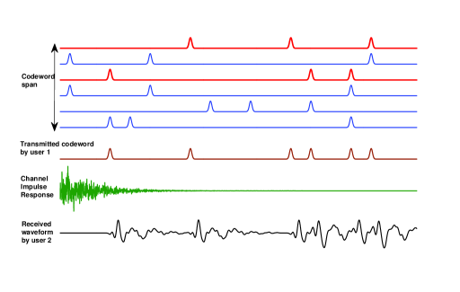
This particular construction of constituent waveforms (codeword span), combinatorial construction of the transmitted signal and the fact that all play a crucial part since they allow very efficient decoding, MAC-less user coordination and full duplex operation for each user. A key feature of the constituent waveforms is sparsity i.e. the waveforms are constructed from very short bursts of digital modulation signals. We emphasize, it is not the digital signal which carries useful information - the information rate is the same no matter what modulation (BPSK, QPSK, 16-QAM etc) we choose to construct the waveforms. It is the choice of the -combination of the codeword span and of the associated weights which carries the information.
The transmitted waveform is propagated in a dispersive channel (depicted as a green line) and received as a convolution of the two (black line). The implicit assumption here is that the channel can be modelled as a linear time invariant channel (FIR filter). Such an assumption is a commonplace in the literature and in practice.
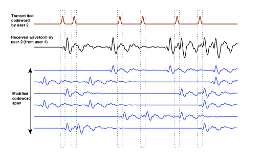
The CCSM method relies on the linearity property of convolution. The receiver reconstructs a modified codeword span – blue waveforms in Figure 2, where each waveform in the original codeword span is convolved with the channel signature. The task for the receiver is to estimate which waveforms were used by the transmitter. The whole detection process can be performed efficiently using sparse recovery solvers. The transmitted waveform is essentially a sequence of on-off duty cycles, where for most of the time there are silent periods (“off cycles”). Each user utilises its “off cycles” to receive signals from the other users. In the “on cycles”, however, the user cannot receive the signal, which represents an erasure in the codebook. This is depicted in Figure 2 as the doted boxes. Only non-erased portions of the codebook are used in the detection process. Technically, with this scheme the Rx/Tx chains do not operate simultaneously. Furthermore, the explicit assumption is that the nodes operate fast switching (at the symbol rate) between Rx/Tx, which is indeed possible with the current RF technology.
II-B Constant Weight Codes
The CCSM requires a non-linear encoding operation. The process of mapping the information vectors at each user to a unique -combination of the codeword span can be viewed as constant (hamming) weight coding (CWC). The problem of efficient encoding and decoding constant-weight vectors received significant interest in the literature. There are practical algorithms of computational complexity linear in the length of constant weight vectors, which are based on lexicographic ordering and enumeration [6]. However, the approach particularly suitable for our system is that of [7], as its complexity is quadratic in the weight of constant weight vectors, which fares favourably in comparison to the enumeration approach in the case where . In [7], authors pursue geometric representation of information vectors in an -dimensional Euclidean space and establish bijective maps by dissecting certain polytopes in this space.
II-C CCSM Encoder
Consider a network of users denoted , each of which has a bit message to transmit to all others through a wireless medium using the same single carrier frequency. Denote by the number of transmissions, and by the message at user . It is assumed that users are equipped with an encoder, which constitutes of bijective maps and . The first map, , maps -bit binary words into an constant weight binary code . The second map assigns complex-numbered values to the non-zero entries in a constant weight binary codeword from . For simplicity, we may assume that consists of all possible constant weight codewords, in which case we can take . Each user is assigned a signaling dictionary , where each is a sparse column vector. (Columns of the matrix can be thought of as sampled waveforms constituting the codeword span in Fig. 1.) Each user has perfect knowledge of all signaling dictionaries. Furthermore, each user has a perfect knowledge of the channel impulse responses of the channel between users and , and of its own channel impulse response , which we refer to as a “self-channel”. (“Self-channel” can be thought of as a “radar return”, and its role is explained in the description of the CCSM decoder.)
We remark that the signalling dictionary at user can be judiciously optimized to suit the preferred choice of system parameters. In the sequel, we will consider the following construction: all columns of have equal number of non-zero entries, set to , and non-zero entries are selected uniformly at random from a predefined constellation, e.g, from the set . Moreover, every two columns in have disjoint support. This way, as the transmitted codeword is formed as a weighted sum of exactly columns in , the transmitted codeword will have exactly non-zero entries, implying that every user will have exactly on-slots and will use its off-slots to listen to the incoming signals of other users. Another way to construct a signalling dictionary would be to apply a regular Gallager construction, which was originally developed for LDPC codes (cf., e.g., Ch. VI of [13] and references therein).
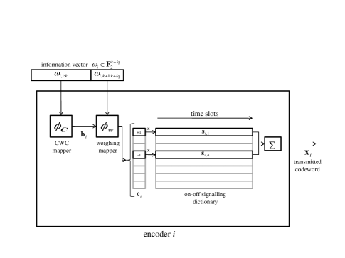
Figure 3 depicts a CCSM encoder at user . The encoding three-step procedure is summarized below222Throughout the paper, for , , denotes the set , and for a vector , and set of indices , .:
-
1.
User encodes using a CWC code.
-
2.
Further bits are encoded on non-zero entries in , i.e., . This is based on a bijective map that assigns a different complex number to each binary sequence of length , which can be thought of as a QAM modulation with constellation points.
-
3.
User transmits , where the matrix-vector multiplication is performed over .
II-D CCSM Decoder
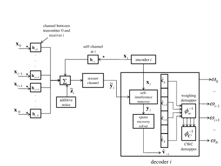
Figure 4 depicts a CCSM decoder at user . The CCSM decoder receives a superposition of all signals from all intended transmitters, i.e., users . As aforementioned, the receiver does not receive the signal in on-cycles (when it transmits), which is represented by the erasure channel. Upon removing the self interference components, the CCSM decoder employs a sparse recovery solver.
Specifically, the recovery at node proceeds as follows:
-
1.
Define an erasure pattern vector as , where if and otherwise. Define an erasure matrix , produced from identity matrix, by removing rows where corresponding has zero entry. Denote the number of rows in by .
-
2.
User using off-duty cycles receives:
(1) where symbol denotes convolution truncated to time slots and represents the additive Gaussian noise over time slots.
-
3.
Since each user switches into reception mode in between transmitting short bursts, there would be echoes of its own transmitted signal in the received signal (self interference). However, all users know their own transmitted signal and can therefore subtract the term in eq. (1) as long as they know the “self channel”.
(2) where , is the -column vector formed by concatenating vertically , ,…, ,,… i.e., and is an matrix, given by:
Note that the matrix can be calculated offline, as it depends only on the channel impulse responses and the signaling dictionaries. Therefore, it needs to be updated only when the channel impulse response changes.
-
4.
User needs to solve the following problem to detect the desired signal:
(4) This is a non-convex optimisation problem. However, we note that exactly out of entries in are non zero, hence its sparsity level is by the initial assumption . This set-up is found in compressive sensing (CS) problems, and thus one can apply a range of efficient sparse recovery solvers available in the literature to find an approximate solution to eq. (4), which we discuss in the next Section.
-
5.
Finally, user decodes the messages for all :
III Sparse Recovery for CCSM
We recall that each user is required to solve the sparse recovery problem (4) in order to correctly detect the transmitted messages. This is a non-convex and intractable optimization problem. However, in the spirit of the compressed sensing framework, one can apply a convex relaxation, by replacing the norm with the norm:
| (5) |
We will refer to the convex relaxation in 5 as Group Basis Pursuit (GBP). Furthermore, one can employ an even simpler form of the convex relaxation, i.e., a standard embodiment of the LASSO/Basis Pursuit (BP):
| (6) |
where the group structure of non-zero entries in is omitted, but can be enforced after solving (6).
Another method to solve our original problem (4), is to employ a greedy iterative sparse recovery algorithm. A number of such algorithms have appeared in the literature including Compressive Sampling Matching Pursuit (CoSaMP) [2] and Subspace Pursuit (SP) [3]. These algorithms can be enhanced to take into account the additional group structure of the unknown vector, which is imposed by our system set-up. Namely, in addition to the unknown vector having non-zero entries, each of its subvectors of length , has exactly non-zero entries. In Algorithm 1, we present the modification of Subspace Pursuit, which we name Group Subspace Pursuit (GSP). For simplicity and without loss of generality, we present the GSP as applied to the sparse recovery problem at user . The GSP is a low complexity method, which has computational complexity of Least Square estimator of size , and is vastly more computationally efficient than convex optimisation based methods, including Group Basis Pursuit (GBP) and Basis Pursuit (BP).
-
•
Input. A waveform at user , received during the off-duty cycles, with the self-interference component removed, CIR/Signaling matrix , CCSM parameters and .
-
•
Output. Vector consisting of subvectors of length , each having exactly non-zero entries.
-
1.
Initialize. Set , , .
-
2.
Identify. For each , set to the indices largest in magnitude in the -th -sub-vector of , i.e.,
-
3.
Merge. Put the old and new columns into one set: .
-
4.
Estimate. Solve the least-squares problem on the chosen column-set:
-
5.
Prune. Retain the coefficients largest in magnitude in each -sub-vector of , i.e.,
to obtain the support estimate
-
6.
Iterate. Find the -th estimate and update the residual:
Set and repeat (2)-(6) until stopping criterion holds.
-
7.
Output. Return .
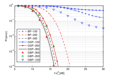
Figure 5 depicts performance of the three sparse solvers for group CS set-up. In this study there are groups, and in each group out of elements are non zero. This investigation was performed for three under sampling ratios for each of those reconstruction methods. For example, BP-100 signifies the Basis Pursuit solver on a Complex Gaussian dense measurement matrix with size (i.e. 31% under sampling ratio). The non-zero elements in the unknown vector are drawn from a QPSK modulation set. The error event is defined as any symbol error in the group. For low under sampling ratios, Group Basis Pursuit performs best. However, for moderate and larger values, our Group Subspace Pursuit is almost the same. Therefore, given its low complexity, we apply GSP to analyse the CCSM performance in the sequel.
IV Numerical results
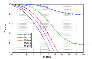
In this section we report numerical results of the proposed method and quantitative comparison with the state-of-the-art. We consider a multi-user wireless network with nodes, where all users are within radio range of each other. All users attempt to broadcast a message to all other nodes. We assume a very dispersive channel, modelled by an FIR filter with 32 taps, with exponentially decaying profile. Moreover, we assume that each pair of nodes has an independent channel. We set , , and use QPSK signalling (), i.e., each message contains bits. Figure 6 depicts the performance of the proposed method for 5 users in terms of message error rate (MER) as a function of signal-to-noise ratio, for various values of the number of available symbol intervals. The MER is an empirical probability estimate of a failure occurring in the message delivery. We remark that the values of MER could be further decreased by the use of outer coding.
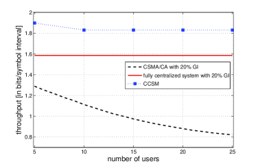
To further assess the performance of the CCSM method, we compare its achieved throughput to the throughput estimates of what would be the best hypothetical solutions, constructed using the state-of-the-art in an idealised scenario. As before, we assume that the transmission occurrs over a time dispersive channel, modelled by an FIR filter with 32 taps, but, in order to make a fair comparison to MAC protocols below, without any additive noise. Achieved throughput of CCSM in bits per symbol interval, given by , where is the minimum number of symbol intervals at which no message errors occurred in at least 100,000 simulation trials, is plotted in Fig. 7. We note that the throughput performance of the CCSM is insensitive to the number of users in the network.
First hypothetical system we consider exploits a central controlling mechanism that closely coordinates transmissions between all users, using a TDMA channel access. To avoid interference the total transmission time would be divided equally into non overlapping slots. Each user would broadcast its message to all other users in its designated slot, and receive messages from all other users in remaining slots. To cope with the dispersive channel nature, such system would need to use FDE/OFDM. A typical FDE/OFDM system requires a guard interval (cyclic prefix) of about 20% slot duration. However, in reality, additional guard intervals would be needed, and close coordination between nodes implies additional overheads. When compared even to this idealised and highly impractical system, our method offers a better throughput, as each message transmission requires symbol intervals, which results in the throughput of bits per symbol interval regardless of the number of users in the network.
However, in most cases, such a central controlling mechanism would be unavailable, and the second, more realistic, benchmarking system we consider is based instead on distributed coordination function (DCF) and CSMA/CA [14], more specifically on DCF as used in IEEE 802.11b MAC in broadcasting mode. Such system relies on the randomised deferment of transmissions in order to avoid collisions on a shared wireless medium. Since we assume that all users are within radio range of each other, there is no inefficiency resulting from hidden/exposed terminals, thus we employ only the basic access mechanism of CSMA/CA protocol. In addition, we assume that each message transmission contains a guard interval of about 20% slot duration to cope with the dispersive channel nature, so that each message transmission requires 41 symbol intervals as above. The minimum and maximum contention windows of CSMA/CA are assumed to consist of 16 and 1024 symbol intervals, respectively. We consider an idealised version of the protocol where no symbol intervals are wasted on distributed or short interframe space (DIFS/SIFS), propagation delay, physical or MAC message headers and ACK responses. Moreover, the transmission queue of each user consists of a single message. Thus, any inefficiency of the scheme is a result either of the idle contention intervals or collisions. The simulated average throughput of such scheme is presented in Fig. 7. We note that CCSM significantly outperforms even such idealised CSMA/CA scheme offering, e.g., twice the throughput of idealised CSMA/CA in the case of 20 users.
V Conclusions
In this paper we have introduced a novel modulation and multiplexing method for ad-hoc wireless networks. The CCSM method offers a range of benefits: same time/frequency duplex, minimal MAC, inherent robustness in time dispersive channels. The CCSM is also applicable to optical communications (both guided and free space), where it could offer better performance/flexibility than combinatorial PPM. We have demonstrated significant data throughput improvements against the state-of-the art. However, the presented performance gains of CCSM are conservative, since we have opted for a low complexity detection method. Further performance gains can be achieved by employing sparse recovery methods which would capitalise on the discrete nature of the unknown signal vector.
References
- [1] Lei Zhang and Dongning Guo “Wireless Peer-to-Peer Mutual Broadcast via Sparse Recovery” preprint available from: http://arxiv.org/abs/1101.0294.
- [2] D. Needell and J. A. Tropp, “CoSaMP: Iterative signal recovery from incomplete and inaccurate samples,” Applied and Computational Harmonic Analysis, vol. 26, pp. 301–321, 2009.
- [3] W. Dai and O. Milenkovic, “Subspace pursuit for compressive sensing signal reconstruction,” IEEE Trans. Inform. Theory, vol. 55, pp. 2230– 2249, 2009.
- [4] D. L. Donoho, “Compressed sensing,” IEEE Trans. Inform. Theory, vol. 52, pp. 1289–1306, 2006.
- [5] E. J. Candes and T. Tao, “Near-optimal signal recovery from random projections: Universal encoding strategies,” IEEE Trans. Inform. Theory, vol. 52, pp. 5406–5425, 2006.
- [6] T.V. Ramabadran, “A coding scheme for m-out-of-n codes,” IEEE Trans. Commun., vol. 48, pp. 1156–1163, 1990.
- [7] C. Tian, V. Vaishampayan and N. J. A. Sloane, “A coding algorithm for constant weight vecotrs: a geometric approach based on dissections,” IEEE Trans. Inform. Theory, vol. 55, pp. 1051–1060, 2009.
- [8] Ewout van den Berg, “Probing the Pareto Frontier for Basis Pursuit Solutions”, SIAM J. Sci. Comput. 31, 890 (2008) ; doi:10.1137/080714488
- [9] H. Sugiyama and K. Nosu, “MPPM: A method of improving the band-utilization efficiency in optical PPM,” J. Lightwave Technol., vol. 7, Mar. 1989.
- [10] J. M. Budinger, M. Vanderaar, P. Wagner and S. Bibyk, “Combinatorial pulse position modulation for power-efficient free-space laser communications,” Proc. SPIE, vol. 1866, 1993.
- [11] C.N. Georghiades, “Modulation and coding for throughput-efficient optical systems,” IEEE Trans. Inform. Theory, vol.40, pp.1313-1326, 1994.
- [12] Li Zhao and A.M. Haimovich, “Multi-user capacity of M-ary PPM ultra-wideband communications,” Proc. IEEE Conf. on Ultra Wideband Systems and Technologies, pp. 175-179, 2002.
- [13] David J.C. MacKay, Information theory, Inference and Learning Algorithms, Cambridge University Press, 2003.
- [14] G. Bianchi, “Performance Analysis of the IEEE 802.11 Distributed Coordination Function”, IEEE Journal on Selected Areas in Communications, vol. 18, pp. 535–547, 2000.