The use of Ansys to calculate sandwich structures

Abstract

In this article, we make a comparative study on a simply supported sandwich beam subjected to a uniform pressure using different modellings offered by the software Ansys 5.3 to compute displacements and stresses.

8 nodes quadrilateral elements Plane 82, multi-layered 8 nodes quadrilateral shell element Shell 91 and multi-layered 20 nodes cubic element Solid 46 are used. Influence of mesh refinement and of ratio of young’s moduli of layers are studied.

Finally, a local Reissner method is presented and assessed, which permits to improve the accuracy of interface stresses for high ratio of young’s moduli of layers using Plane 82 elements.

1 Introduction

Sandwich materials really begin to be highly appreciated in the industry, and especially in the field of transport (automotive, aeronautics, shipbuilding and railroads) or in civil engineering.

It is therefore important to determine which elements should be used to model such structures.

A sandwich structure is composed of three layers:

• two edges made of rigid layers, working in membrane, which represent the skins;

• a thick and soft central layer, the core, with low rigidity and density and essentially submitted to transverse shear loading, is sandwiched in between the edges.

In the design process, interface stresses can be of great importance, since they play a crucial role in failure modes, as explained in [1, 2].

The core being essentially subjected to transverse shear stress, this component, which is generally very much lower than the others, must not be neglected: in some cases, effects arising from shear effects overhang others phenomena (flexural effects for example), as shown for example in [3, 4, 5, 6].

The determination of transverse shear stress at interfaces is therefore of particular importance in the design of new optimized materials.

If we assume that the three layers remain perfectly bonded, then at interfaces:

• the displacement field must be continuous;

• the normal trace of the stress must be continuous.

In this article, we shall study a very simple case using the famous finite element software Ansys 5.3. We shall not talk about special elements based on hybrid [7, 8], mixed [9, 10, 11, 12] or modified [13, 14, 15] formulation nor about pre- and post-processing methods [16, 17].

Solutions obtained with different modellings (complex or simple ones) are compared. Particular emphasis is put on their respect of continuity requirements.

By modifying the stiffness of the core, we shall see which modelling should be preferred by designers.

Finally a method, based on Reissner’s formulation, is developed to improve the accuracy for new sandwiches.

2 Description of the study

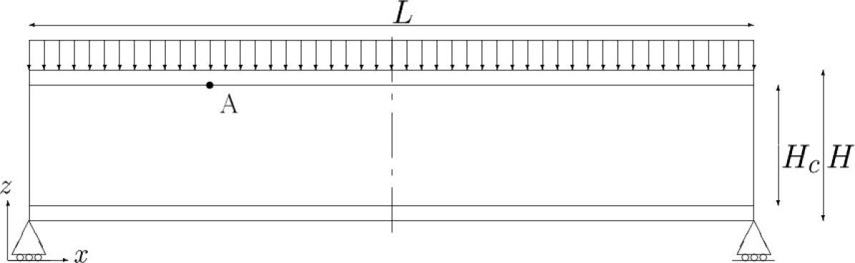
Figure 1: Sandwich beam

One of the most simple example is the case of the simply supported sandwich beam subjected to an uniform pressure on its top face. This beam is shown in figure 1.

2.1 Characteristics

The geometry is defined as follows:

• The total length of the beam is $L=24$ mm;

• its total height $H=2$ mm, the core representing 80% of the total height of this symmetrical sandwich, each skin is $0.2$ mm height;

• the thickness of the beam is equal to unity.

The applied pressure is $q=-1$ N/mm.

2.2 Parameters of the study

In this study, we are interested in determining the structural response at point A (at the interface between the top skin and the core and located at $x_{1}=L/4$) when different parameters vary.

Skins are made of aluminum ($E_{s}=70000$ MPa and $\nu_{p}=0.34$). The core will be:

• Case A: of carbon/epoxy ($E_{c}=3400$ Mpa and $\nu_{c}=0.34$);

• Case B: of foam ($E_{c}=340$ Mpa and $\nu_{c}=0.40$);

• Case C: of soft foam ($E_{c}=70$ Mpa and $\nu_{c}=0.40$);

• Case D: other material: $\nu_{c}=0.4$ is fixed and $E_{s}/E_{c}$ varies.

2.3 The modellings

By symmetry, only one half of the beam is modelled.

Before building the different modellings, we define the following parameters for the meshing:

• $ncuts$: number of longitudinal cuts (in the beam’s axis direction);

• $nskin$: number of elements in the thickness of each skin;

• $ncore$: number of elements in the thickness of the core.

We shall use the following modellings:

• the reference modelling:

  • 2D using the 8 nodes quadrilateral element Plane 82;

  • 4 elements through the thickness of each skin ($nskin=4$), 32 through the thickness of the core ($ncore=32$), and 400 longitudinal cuts ($ncuts=400$) in the beam’s axis directions (16000 elements for the half beam);

  This fine meshing yields to the exact solution given by [18].

• a planar modelling using the plane element Plane 82:

  1 element is used to model each layers (nskin = ncore = 1), i.e. 3 elements through the thickness of the sandwich;

• a modelling using the multi-layered cubic element Solid 46:

  1 element through the total thickness representing all the layers of the sandwich structure;

• one modelling done with the multi-layered shell element Shell 91, with sandwich option (keyopt(9)=1):

  1 element through the total thickness representing all the layers of the sandwich structure.

2.4 Results of interest

In our studies, we shall focus on the following results of particular interest:

• the maximum displacement of the structure in $z$ direction, denoted $U_{z}$ in results;

• the discontinuous components of stresses, $\sigma_{xx}$, at point A in the skin and in the core, and the continuous component $\sigma_{zz}$;

• interlaminar stress: this is the continuous component $\sigma_{xz}$ at point A.

3 Study of the sandwich beam

We now present results obtained with Ansys 5.3 and corresponding to different materials and different meshes.

3.1 Influence of ncuts on the different modellings

In this section, we are interested in the structural responses to the different modellings for $E_{c}=3400$ MPa, $E_{c}=340$ MPa and $E_{c}=70$ MPa.

Results concerning the case $E_{c}=340$ MPa are plotted in figures 2 for displacements, 3 and 4 for the two continuous components $\sigma_{zz}$ and $\sigma_{xz}$ and 5 and 6 for $\sigma_{xx}$ in the core and in the skin respectively.

Tables 1, 2 and 3 present numerical results and error percentages after convergence for these 3 cases.

From these figures and tables, the following conclusions can be drawn:

• Plane 82 is very much better than others modellings. Nevertheless, it is to be noticed that it seems to diverge for displacements (with the coarse mesh used: $nskin=ncore=1$);

• Solid 46 is the worst model. It never converges towards the right values (for any component of stresses nor for displacements);

• Shell 91 is particularly interesting for continuous components of stresses $\sigma_{zz}$ and $\sigma_{xz}$;

• Plane 82 is the only modelling leading to a correct determination of the discontinuous component $\sigma_{xx}$ in the skin and the core;

• It seems that errors increase with the ratio $E_{s}/E_{c}$. This point will be studied in the next section.

3.2 Influence of ratio $E_{s}/E_{c}$ for ncuts=20

Since every material which can be obtained in a thin skin shape is acceptable for the skins and every material with low density is acceptable for the core, sandwich materials cover an extremely wide domain.

A parameter of interest is therefore the ratio of young’s moduli $E_{s}/E_{c}$. This parameter can vary from 4 (old sandwiches, so to speak, very close to laminates) to 1000 (some new high-tech sandwiches developed for very particular applications go up to 1500). But we must remark that sandwiches often exhibit a ratio greater than 200.

In this section we shall study the influence of this ratio on the different modellings when the utilized mesh is fixed to $ncuts=20$.

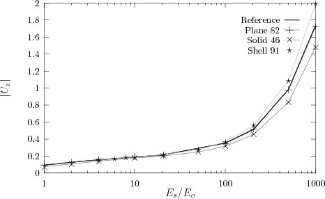
Figure 7: Influence of $E_{s}/E_{c}$: $U_{z}$ ($ncuts=20$)

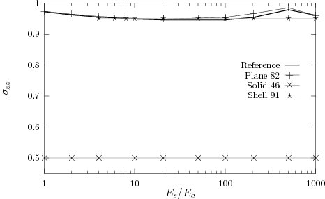
Figure 8: Influence of $E_{s}/E_{c}$: $\sigma_{zz}$ ($ncuts=20$)

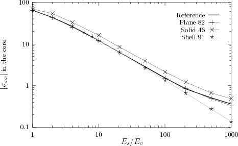
Figure 10: Influence of $E_{s}/E_{c}$: $\sigma_{xx}$ in the core ($ncuts=20$)

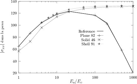
Figure 11: Influence of $E_{s}/E_{c}$: $\sigma_{xx}$ in the top skin ($ncuts=20$)

Results concerning displacements are plotted in figure 7. Continuous components $\sigma_{zz}$ and $\sigma_{xz}$ are shown in figures 8 and 9. The discontinuous component $\sigma_{xx}$ is illustrated in figures 10 and 11 in the core and in the skin respectively.

From these figures, the following conclusions can be drawn:

• Plane 82 is the best modelling for displacements, $\sigma_{zz}$ and $\sigma_{xx}$ in the core and the skin;

• Shell 91 and Solid 46 are acceptable for displacements and $\sigma_{xx}$ in the core. They are acceptable for $\sigma_{xx}$ in the skin for $E_{s}/E_{c}\leq$ 50;

• Shell 91 leads to an acceptable approximation of $\sigma_{zz}$, and is very interesting for $\sigma_{xz}$;

• Plane 82, which was exceptionally good in the last section, shows some difficulty here, especially at high $E_{s}/E_{c}$ ratio for $\sigma_{xz}$. The influence of the meshing of the beam with Plane 82 elements is studied in the next section.

3.3 Element Plane 82: influence of mesh refinement

In previous sections, the mesh corresponding to the 8 nodes quadrilateral element Plane 82 only used 1 element to model 1 layer.

We propose to see what happens when the number of elements through the thickness of the skins ($nskin$) and of the core ($ncore$) vary.

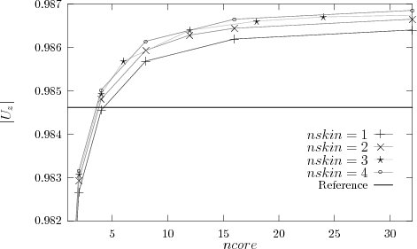
Figure 12: Influence of nskin and ncore: $U_{z}$ ($ncuts=20$ and $E_{s}/E_{c}=500$)

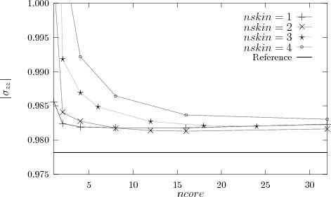
Figure 13: Influence of nskin and ncore: $\sigma_{zz}$ ($ncuts=20$ and $E_{s}/E_{c}=500$)

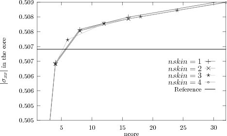
Figure 15: Influence of nskin and ncore: $\sigma_{xx}$ in the core ($ncuts=20$ and $E_{s}/E_{c}=500$)

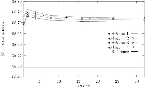
Figure 16: Influence of nskin and ncore: $\sigma_{xx}$ in the top skin ($ncuts=20$ and $E_{s}/E_{c}=500$)

Displacements are plotted in figure 12, $\sigma_{zz}$ and $\sigma_{xz}$ in figures 13 and 14, and $\sigma_{xx}$ in figures 15 and 16 in the core and in the skin respectively. These computations are done for a ratio $E_{s}/E_{c}=500$.

From these figures, the following conclusions can be drawn:

• results are always accurate when $ncore=8\ nskin$, i.e. when the meshing is regular through the thickness;

• $nskin$ and $ncore$ do not have any influence on the convergence of displacements, essentially due to flexion: the number of longitudinal cuts, $ncuts$, is therefore the most preponderant parameter.

• a very refined mesh ($nskin=4$ and $ncore=8\ nskin$) must be used in order to converge towards the right value of $\sigma_{zz}$;

• a coarse mesh ($nskin=1$) does not permit to obtain an acceptable value of $\sigma_{xz}$;

• convergence towards $\sigma_{xx}$ reference value in the core is controlled by ncuts. Results are not improved by increasing $nskin$ nor $ncore$;

• the last point is also true for the convergence towards $\sigma_{xx}$ value in the skin.

4 Local Reissner: improving results for Plane 82

As it can be see from figure 9 and from table 4 (which summaries results and gives the good “working zone” of the different modellings), Plane 82 is not able to give accurately the interlaminar stress $\sigma_{xz}$ with a coarse mesh. Since this component is very important in the design process, results must be improved.

A way of improving results is to refine the meshing. In figure 9, the curve ‘Plane 82/2’ gives results obtained with $nskin=1$ and $ncore=2$ (instead of 1). This slightest modification of the mesh (4 elements through the thickness of the sandwich instead of 3) is sufficient to lead to very good results for $E_{s}/E_{c}\leq 200$.

But, as mentioned before, sandwiches nowadays exhibit ratios generally higher than 200. In this range, the convergence is only reached with a very refined meshing: $nskin\geq 3$ and $ncore=8\ nskin$. Such a mesh yields an unacceptable computation time.

In order to improve the accuracy of stresses, we must answer to the following question: how are nodal stresses computed?

Nodal stresses $\mathbf{\boldsymbol{\tau}}$ are generally computed using a minimization process. They are obtained from nodal displacements $\mathbf{\boldsymbol{q}}$ using a least squares method and by minimizing:

$$\int_{\Omega}\left(\mathbf{\boldsymbol{\sigma_{m}}}-\mathbf{\boldsymbol{\sigma_{u}}}\right)^{2}\ \d\Omega$$ (1)

where $\mathbf{\boldsymbol{\sigma_{m}}}$ denotes the mixed way to calculate stresses:

$$\mathbf{\boldsymbol{\sigma_{m}}}=\mathbf{\boldsymbol{N_{\sigma}}}\mathbf{\boldsymbol{\tau}}$$ (2)

and $\mathbf{\boldsymbol{\sigma_{u}}}$ the displacements way:

$$\mathbf{\boldsymbol{\sigma_{u}}}=\mathbf{\boldsymbol{D}}\mathbf{\boldsymbol{\mathcal{L}}}\mathbf{\boldsymbol{N_{u}}}\mathbf{\boldsymbol{q}}$$ (3)

or using the stress projection method presented in [19] by minimizing:

$$\int_{\Omega}\left(\mathbf{\boldsymbol{\sigma_{m}}}-\mathbf{\boldsymbol{\sigma_{u}}}\right)\ \d\Omega$$ (4)

In these equations, $\mathbf{\boldsymbol{D}}$ is the generalized Hooke’s matrix relating stresses to strains, $\mathbf{\boldsymbol{\mathcal{L}}}$ the differential operator relating strains to displacements, $\mathbf{\boldsymbol{N_{\sigma}}}$ and $\mathbf{\boldsymbol{N_{u}}}$ the matrices of shapes functions for stresses and displacements, and $\Omega$ the volume or surface of interest.

It is to be noticed that these methods lead to convergence towards Reissner’s (reference) solution.

As expressed in [20], the minimization process can be global (done over the whole structure: $\Omega$ being the entire structure) or local (done over one element: $\Omega$ being the considered element). Since the local process converges towards the same limit as the global process, the minimization process chosen is generally the local one.

Nevertheless, instead of minimizing the difference between two solutions, it may be more convenient (simpler and faster) to directly find the stress field using Reissner’s formulation.

In Reissner’s solution, nodal stresses are related to nodal displacements by [21, 22, 23, 24]:

$$\mathbf{\boldsymbol{\tau}}=\mathbf{\boldsymbol{A}}^{-1}\mathbf{\boldsymbol{B}}\mathbf{\boldsymbol{q}}$$ (5)

with:

$$\mathbf{\boldsymbol{A}}=+\displaystyle\int_{\Omega}{}^{t}\!\mathbf{\boldsymbol{N_{\sigma}}}\mathbf{\boldsymbol{S}}\mathbf{\boldsymbol{N_{\sigma}}}\ d\Omega$$ (6)

and

$$\mathbf{\boldsymbol{B}}=+\displaystyle\int_{\Omega}{}^{t}\!\mathbf{\boldsymbol{N_{\sigma}}}\mathbf{\boldsymbol{\mathcal{L}}}\mathbf{\boldsymbol{N_{u}}}\ d\Omega$$ (7)

$\mathbf{\boldsymbol{S}}=\mathbf{\boldsymbol{D}}^{-1}$ being the compliance matrix.

In order to improve the stress computation at interfaces, we propose to use the last formulation on two adjacent elements, located on each side of an interface. Doing so, we ensure the equilibrium state at interface on a better way. We shall refer to this method as “local Reissner” method.

This kind of method is not more time consuming than least squares methods generally used (in Ansys for example) to derive nodal stresses from nodal displacements.

Now looking at figure 17, which is a close-up view of figure 9 for sandwiches with $E_{s}/E_{c}\geq 200$, we can see that:

• the use of local Reissner’s method (denoted Local Reissner/2 because we used $ncore=2$) permits to really improve the accuracy of $\sigma_{xz}$, which is of great importance.

• It is to be noticed that the same mesh with Plane 82 (Plane 82/2) does not permit to improve results with this high $E_{s}/E_{c}$ ratio.

• The solution given by Shell 91 is not so good as for lower $E_{s}/E_{c}$ ratio.

5 Conclusions

The reference solution has been obtained using a very fine meshing and the 8 node quadrilateral element Plane 82 in order to reach the analytical solution of Pagano [18].

The first study, influence of ncuts on the different modelling in section 3.1, seems to lead to the conclusion that Plane 82 is the best model, specially when looking at figures 2-6 (obtained with a coarse mesh and in the case $E_{s}/E_{c}\approx 200$). Nevertheless, the study of the influence of the $E_{s}/E_{c}$ ratio in section 3.2 permits to see some weakness of this model.

In terms for design quantities:

• all models leads to a correct value of displacements, but Plane 82 is the most accurate;

• $\sigma_{zz}$ can be correctly given by Shell 91 and Plane 82, the latest being the most accurate;

• $\sigma_{xz}$ is only very accurately computed with Shell 91, but for $E_{s}/E_{c}\leq 200$;

• $\sigma_{xx}$ in the core can be calculated using any model, Plane 82 being the most accurate;

• $\sigma_{xx}$ in the skin is very accurately computed with Plane 82 and with Shell 91 (but only for $E_{s}/E_{c}\leq 20$), and acceptable with Solid 46 (and only for $E_{s}/E_{c}\leq 20$).

A summary of results, and the “working zone” in which the different elements can be used is given in table 4.

Hence, from the previous results, we can say that:

• for planar problems, Plane 82 is very well adapted. Nevertheless, it is to be noticed that this method is not very stable for very coarse meshes (small values of $nskin$, $ncore$ and $ncuts$), and that interlaminar stress $\sigma_{xz}$ can only be reached with a fine meshing;

• Shell 91 (with sandwich option) is a good way of computing sandwich structures. Nevertheless if the designer must know $\sigma_{xx}$ at interfaces, then this element can only be used for $E_{s}/E_{c}\leq 50$.

• Solid 46 is not very accurate in the determination of the design quantities. A model using this kind of element should be avoided. Nevertheless, it is to be noticed that this element has not been developed to perform such computations (high differentce of stiffness between layers).

The presented local Reissner’s method permits to reach excellent results, especially for the interlaminar stress $\sigma_{xz}$ and for $E_{s}/E_{c}\geq 200$ with a coarse mesh through the thickness of the sandwih. We can notice that such a meshing, with 4 elements through the thickness of the sandwich yields results very closed to the exact solution obtained with 40 elements through the thickness!

This method is particularly interesting for the design of new sandwich materials.

Finally, we want to put emphasis on the fact that this method is particularly easy to implement, as a stand-alone program, but also in existing finite element softwares.

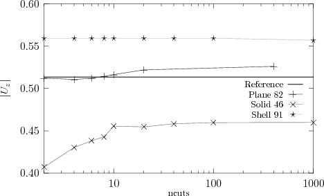
Figure 2: Influence of ncuts: $U_{z}$ (case B)

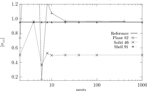
Figure 3: Influence of ncuts: $\sigma_{zz}$ (case B)

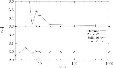
Figure 4: Influence of ncuts: $\sigma_{xz}$ (case B)

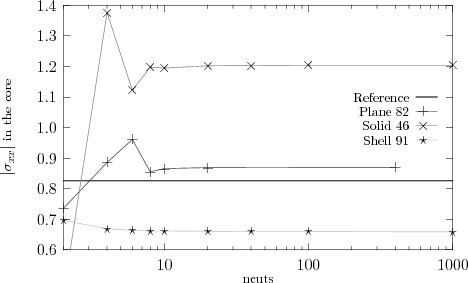
Figure 5: Influence of ncuts: $\sigma_{xx}$ in the core (case B)

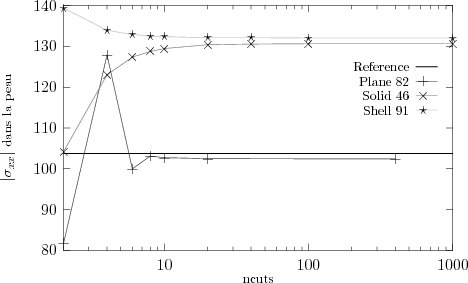
Figure 6: Influence of ncuts: $\sigma_{xx}$ in the top skin (case B)

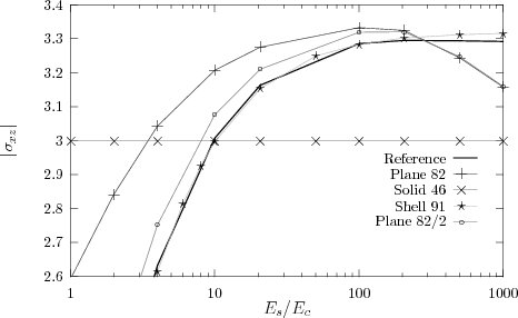
Figure 9: Influence of $E_{s}/E_{c}$: $\sigma_{xz}$ ($ncuts=20$)

Figure 14: Influence of nskin and ncore: $\sigma_{xz}$ ($ncuts=20$ and $E_{s}/E_{c}=500$)

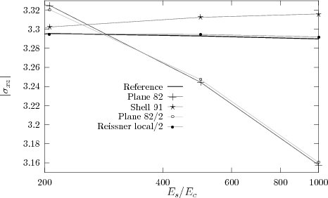
Figure 17: Influence of high $E_{s}/E_{c}$ ratio: $\sigma_{xz}$ ($ncuts=20$)

Table 1: Case A: $E_{c}=3400$ Mpa

	$|U_{z}|$	$|\sigma_{zz}|$	$|\sigma_{xz}|$	$|\sigma_{xx}|$	$|\sigma_{xx}|$	ncuts
				skin	core
Ref	0.21596	0.94624	3.1635	123.13	6.2844
P82	0.21527	0.95033	3.2616	123.08	6.2843	400
	0.319%	0.432%	3.10%	0.04%	0.001%
S91	0.21388	0.90000	3.1587	126.35	6.1369	1000
	0.963%	4.887%	0.15%	2.61%	2.35%
S46	0.20355	0.50000	3.0000	123.28	8.4202	1000
	5.746%	47.16%	5.17%	0.12%	34.0%

Table 2: Case B: $E_{c}=340$ Mpa

	$|U_{z}|$	$|\sigma_{zz}|$	$|\sigma_{xz}|$	$|\sigma_{xx}|$	$|\sigma_{xx}|$	ncuts
				skin	core
Ref	0.51353	0.95461	3.2956	103.71	0.8262
P82	0.52618	0.96321	3.3091	102.38	0.8701	400
	2.463%	0.901%	0.41%	1.28%	5.31%
S91	0.55712	0.90000	3.3024	132.09	0.6599	1000
	8.488%	5.721%	0.22%	27.4%	20.1%
S46	0.45994	0.50000	3.0000	130.68	1.2042	1000
	10.44%	47.62%	8.97%	26.0%	45.7%

Table 3: Case C: $E_{c}=70$ Mpa

	$|U_{z}|$	$|\sigma_{zz}|$	$|\sigma_{xz}|$	$|\sigma_{xx}|$	$|\sigma_{xx}|$	ncuts
				skin	core
Ref	1.740	0.96121	3.2926	20.43	0.3614
P82	1.741	0.96847	3.1561	20.77	0.3301	400
	0.06%	0.755%	4.15%	1.66%	8.66%
S91	1.987	0.90000	3.3161	132.64	0.1364	1000
	14.2%	6.368%	0.71%	549 %	62.2%
S46	1.506	0.50000	3.0000	131.43	0.4802	1000
	13.4%	47.98%	8.89%	543 %	32.9%

Table 4: Accuracy of results (ncuts $\geq 20$ understood)

	$U_{z}$	$\sigma_{zz}$	$\sigma_{xz}$	$\sigma_{xx}$	$\sigma_{xx}$
				core	skin
P82	always good	always good	acceptable for $E_{s}/E_{c}\in[100,400]$	always good	always good
	improvement of results
	– use a fine meshing: $nskin\geq 3$ and $ncore=8\ nskin$
	– use local Reissner’s method
S91	always acceptable	always acceptable	always good	good for $E_{s}/E_{c}\leq 100$	good for $E_{s}/E_{c}\leq 20$
S46	always acceptable	never acceptable	acceptable for $E_{s}/E_{c}\in[8,15]$	always weak	acceptable for $E_{s}/E_{c}\leq 20$

References

- [1] Teti, R. and Caprino, G., Mechanical behavior of structural sandwiches. Sandwich Construction 1, K.-A. Olsonn and R.P. Reichard editors, Chameleon Press LTD., London, 1989, 53-67.
- [2] Couvrat, P., Le collage structural moderne. Théorie & pratique. TEC & DOC – Lavoisier, Paris, 1992.
- [3] Zenkert, D., An introduction to Sandwich Construction. Chameleon Press LTD., London, 1995.
- [4] Allen, H.G., Analysis and Design of Structural Sandwich Panels. Pergamon Press, Oxford, 1969.
- [5] Allen, H.G., Sandwich Construction Today and Tomorrow. Sandwich Constructions 1, K.-A. Olsonn and R.P. Reichard editors. Chameleon Press LTD., London, 1989, 3-23.
- [6] N.J. Hoff. Sandwich Construction, John Wiley & Sons, New-York, 1966.
- [7] Manet, V. and Han, W.-S., La modélisation des plaques sandwich par éléments finis hybrides et ses applications. Actes du troisième colloque national en calcul des structures 2, B. Peseux, D. Aubry, J.-P. Pelle, and M. Touratier editors, Presses académiques de l’Ouest, Nantes, 1997, 657-663.
- [8] Manet, V., Han, W.-S. and Vautrin, A., Static analysis of sandwich plates by finite elements. Proc. EUROMECH 360, Mechanics of Sandwich Structures, Kluwer academic press, Dordrecht, to appear, 1997.
- [9] Aivazzadeh, S.M., Ramahefarison, E. and Verchery, G., Composite structure analysis with micro-computer using classical and interface finite elements. Computers & Mathematics with Applications 11 (10), 1985, 1023-1043.
- [10] Aivazzadeh, S.M. and Verchery, G., Stress analysis at the interface in the adhesive joint by special finite elements. Int. J. Adhesion and Adhesive 6 (4), 1986, 185-188.
- [11] Bichara, M., Sarhan-Bajbouj, A. and Verchery, G., Mixed plane finite elements with application to adhesive joint analysis. Proc. of the European Mechanics Colloqium 227, Mechanical bejaviour of the adhesive joints, 1987, 571-578.
- [12] Lardeur, P. and Batoz, J.L., Composite plate analysis using a new discrete shear triangular finite element. Int. J. Num. Meth. in Eng. 27 (2), 1989, 343-360.
- [13] Verchery, G., Extermal theorems in mixed variables. Application to beam and plates subjected to transverse shears. 15th Polish solid mechanics conference, Zakopane, Sept. 1973.
- [14] Pham Dang, T. and Verchery, G., Analysis of Anisotropic Sandwich Plates Assuring the Continuities of Displacements and Transverse Stresses at the Interfaces, A.S.M.E., 1978.
- [15] El Shaikh, M.S., Nor, S. and Verchery, G., Equivalent material for the analysis of laminated and sandwich structures. ICCM 3, Advances in Composite Materials 2, Pergamon Press, Oxford, 1980, 1783-1795
- [16] Pai, P.F., A new look at shear correction factors and warping functions of anisotropic laminates. Int. J. Solids Structures 32 (16), 1995, 2295-2313.
- [17] Lerooy, J.-F. Calcul des contraintes de cisaillement transversales dans les structures modérement épaisses, Institut National Polytechnique de Lorraine, Nancy, France, 1983.
- [18] Pagano, N.J., Exact solutions for rectangular bidirectional composites and sandwich plates, J. Composite Materials 4, 1970, 20-34.
- [19] Zienkiewicz, O.C. and Taylor, R.L., The Finite Element Method, Vol. 1. MacGraw-Hill, London, 1994.
- [20] Hinton, E. and Campbell, J.S., Local and global smoothing of discontinuous finite element functions using a least squares method. Int. J. for Num. Meth. in Eng. 8, 1974, 461-480.
- [21] Reissner, E., On a variational theorem in elasticity. J. Maths and Physics 29, 1950, 90-95.
- [22] Reissner, E.A., A consistent treatment of transverse shear deformation in laminated anisotropic plates. AIAA J. 10 (5), 1961, 716-718.
- [23] Reissner, E., On the theory of transverse bending of elastic plates. Int. J. Solids Struc. 12, 1976, 545-554.
- [24] Washizu, K., Variational methods in elasticity and plasticity, Pergamon Press, Oxford, 1982.