Quasi-stars, giants and the Schönberg–Chandrasekhar limit

Abstract

The Schönberg–Chandrasekhar (SC) limit is a well-established result in the understanding of stellar evolution. It provides an estimate of the point at which an evolved isothermal core embedded in an extended envelope begins to contract. We investigate contours of constant fractional mass in terms of homology invariant variables $U$ and $V$ and find that the SC limit exists because the isothermal core solution does not intersect all the contours for an envelope with polytropic index $3$. We find that this analysis also applies to similar limits in the literature including the inner mass limit for polytropic models of quasi-stars. Consequently, any core solution that does not intersect all the fractional mass contours exhibits an associated limit and we identify several relevant cases where this is so. We show that a composite polytrope is at a fractional core mass limit when its core solution touches but does not cross the contour of the corresponding fractional core mass. We apply this test to realistic models of helium stars and find that stars typically expand when their cores are near a mass limit. Furthermore, it appears that stars that evolve into giants have always first exceeded an SC-like limit.

1 Introduction

Once the core of a main-sequence star has exhausted its supply of hydrogen, it ceases to produce nuclear energy and, in the limit of thermal equilibrium, becomes isothermal. Schönberg & Chandrasekhar (1942) showed that, if the envelope is polytropic with index $n=3$, then there is a maximum fractional mass that the core can achieve. If the core is less massive, it can remain isothermal while nuclear reactions continue in a surrounding shell. If this mass is exceeded then the core contracts until it is supported by electron degeneracy pressure or helium begins to burn at the centre. The idealised result is sufficiently accurate that it has become a well-established element of the theory of the post-main sequence evolution of stars. It is referred to simply as the Schönberg–Chandrasekhar (SC) limit.

Similar limits have been computed for other polytropic solutions. Beech (1988) calculated the corresponding limit for an isothermal core surrounded by an envelope with $n=1$. Eggleton, Faulkner & Cannon (1998) found that, when $n=1$ in the envelope and $n=5$ in the core, a fractional mass limit exists if the density decreases discontinuously at the core-envelope boundary by a factor exceeding 3. They went further to propose conditions on the polytropic indices of the core and envelope that lead to fractional mass limits. We refer to all these limits, including the original result of Schönberg & Chandrasekhar (1942) as SC-like limits.

Previously, we found that the black hole mass of a polytropic quasi-star exhibits a robust fractional limit (Ball et al., 2011). We have determined why this limit exists in terms of contours of fractional core mass of solutions when plotted in the space of homology invariant variables $U$ and $V$. We have further found that all SC-like limits are explained by a similar approach. In this work, we present our analysis, which unifies SC-like limits and indicates that they exist in a wider range of circumstances than the handful of cases discussed in the literature. In Section 2, we provide a thorough exposition of the relevant features of the $U$–$V$ plane. Readers who are familiar with these details can proceed to Section 3, where we present our new interpretation of SC-like limits. In Section 4, we provide a description that captures all the SC-like limits of Section 3. We also consider how to determine whether a star has reached an SC-like limit and how the fractional mass contours constrain its evolution and we conclude in Section 5.

2 The $U$–$V$ plane

This work rests on the behaviour of solutions in the $U$–$V$ plane so we begin with a review of its features. We derive the Lane–Emden equation (LEE) from hydrostatic equilibrium and mass conservation, introduce homology invariant variables $U$ and $V$ and explain their physical meaning, present the homology invariant transformation of the equation and study the behaviour of its solutions in the $U$–$V$ plane. We hope that, by presenting concisely the details of the $U$–$V$ plane in a context where it is usefully applied, we might remove its stigma as ‘that gruesome tool’.

2.1 The Lane-Emden Equation

Consider the equations of mass conservation,

$$\frac{dm}{dr}=4\pi r^{2}\rho\text{,}$$ (1)

and hydrostatic equilibrium,

$$\frac{dp}{dr}=-\frac{Gm\rho}{r^{2}}\text{,}$$ (2)

where $r$ is the distance from the centre of the star, $m$ is the mass within a concentric sphere of radius $r$, and $p$ and $\rho$ are the pressure and density, respectively. We make the usual polytropic assumption that the pressure and density are related by $p=K\rho^{1+\frac{1}{n}}$, where $n$ is the polytropic index and $K$ is a constant of proportionality. We define the dimensionless temperature $\theta$ by $\rho=\rho_{c}\theta^{n}$, where $\rho_{c}$ is the density at the centre of the star, the dimensionless radius $\xi$ by $r=\eta\xi$, where

$$\eta^{2}=\frac{(n+1)K}{4\pi G}\rho_{c}^{\frac{1}{n}-1}\text{,}$$ (3)

and the dimensionless mass $\phi$ by $m=4\pi\eta^{3}\rho_{c}\phi$.

We use a polytropic equation of state to approximate a fluid that is between the adiabatic and isothermal limits. Shallower temperature gradients correspond to larger effective polytropic indices and the isothermal case (zero temperature gradient) corresponds to $n=\infty$. In this case, the equation of state must be approximated differently but the limit is well-defined when working in the $U$–$V$ plane.

Certain conditions inside a star correspond to certain values of $n$. In convective zones, the temperature gradient is approximately adiabatic, so an ideal gas without radiation has $n=3/2$ and pure radiation has $n=3$. Real stars are more radiation-dominated towards the centre and $n$ varies between these limiting values in convection zones. In radiative zones, $n$ depends on the opacity. It can be shown, for example, that for a polytropic model with uniform energy generation and a Kramer’s opacity law, $n$ ranges from $13/4$ for a pure ideal gas to $7$ for pure radiation (Horedt, 2004). Nuclear burning shells and ionisation regions have shallow temperature gradients and therefore large values of $n$. Thus, the effective polytropic index can vary widely within a star.

Introducing the dimensionless mass, temperature and radius into equations (1) and (2) allows us to write

$$\frac{d\phi}{d\xi}=\xi^{2}\theta^{n}$$ (4)

and

$$\frac{d\theta}{d\xi}=-\frac{1}{\xi^{2}}\phi\text{.}$$ (5)

By differentiating equation (5) and substituting for $d\phi/d\xi$ from equation (4), we arrive at the LEE,

$$\frac{1}{\xi^{2}}\frac{d}{d\xi}\left(\xi^{2}\frac{d\theta}{d\xi}\right)=-\theta^{n}\text{,}$$ (6)

in its usual form as a single second-order ordinary differential equation. Here, we prefer to express it as two first-order equations (4 and 5) because this preserves the physical meaning of the equations and easily permits arbitrary boundary conditions for the inner mass and radius.

Solutions of the LEE which are regular at the centre have $\xi_{c}=\phi_{c}=0$. The subset of solutions that extend from the centre to infinite radius or the first zero of $\theta$ are polytropes of index $n$. We refer to solutions that are regular at the centre but truncated at some finite radius as polytropic cores. Conversely, solutions that extend from a finite radius to infinity or the first zero of $\theta$ are polytropic envelopes. In addition, we refer to models that match polytropic cores to polytropic envelopes as composite polytropes. For $n<5$ polytropes are finite in both mass and radius while for $n>5$ they are infinite in mass and radius. The case $n=5$ represents the threshold between the two: it has a finite mass but infinite radius.

2.2 Homology Invariant Variables

It is known (see Chandrasekhar, 1939) that, if $\theta(\xi)$ is a solution of the LEE, then $\theta^{\prime}(\xi^{\prime})=C^{\frac{2}{n-1}}\theta(C\xi)$, where $C$ is an arbitrary constant, is also a solution. The two solutions are homologous; the similarity between them is called homology. By choosing variables that are invariant under this transformation, we can formulate the LEE as a single first-order equation that captures all essential behaviour. We use the variables

$$U=\frac{d\log m}{d\log r}=\frac{3\rho}{\bar{\rho}}$$ (7)

and

$$V=-\frac{d\log p}{d\log r}=\frac{Gm}{r}\frac{\rho}{p}\text{,}$$ (8)

where $\bar{\rho}=3m/4\pi r^{3}$ is the mean density of the material inside $r$. Although we have defined $U$ and $V$ to reduce the order of the LEE, the corresponding physical definitions make them meaningful for discussions of any stellar model. We make a brief excursion to explain these definitions.

The physical variables are all positive so only the first quadrant ($U,V>0$) of the $U$–$V$ plane is of interest. The variable $U$ is three times the ratio of the local density to the mean density inside that radius. As $r\to 0$, we also have $\rho\to\bar{\rho}$ and thus $U\to 3$. We expect that the density of a stellar model decreases with radius, so $\rho/\bar{\rho}<1$ and hence $U<3$. The variable $V$ is related to the ratio of specific gravitational binding energy to specific internal energy. At the centre, $p$ and $\rho$ are finite and $m\sim\frac{4\pi}{3}\rho r^{3}$, so $V\to 0$. Thus, in all physical solutions that extend to $r=0$, the centre corresponds to $(U,V)=(3,0)$. If an interior solution has $V$ everywhere smaller than the appropriate polytrope then it behaves as if it has a finite point mass at its centre. Huntley & Saslaw (1975) referred to similar models, integrated outwards from a finite radius, as loaded polytropes. If a solution has $V$ everywhere greater than the polytrope then it reaches zero mass before zero radius. Such solutions would have a massless core with finite radius, which is unphysical. At the surface, $\rho\to 0$ so $U\to 0$ too. On the other hand, $Gm/r$ takes a finite value but $p/\rho\propto T\to 0$ so $V\to\infty$. All realistic models, be they polytropes, composites of a polytropic core and envelope, or output from a detailed calculation, must adhere to these central and surface conditions in the $U$–$V$ plane. They therefore extend from $(3,0)$ towards $(0,\infty)$. Fig. 1 shows this behaviour for polytropes of indices $1$, $3$, $5$ and $\infty$. The $n=1$ and $n=3$ models extend properly to the surface. The $n=5$ and $\infty$ polytropes do not and therefore cannot represent a real star. In addition, we have plotted a $1\hbox{$\,\text{M}_{\sun}$}$ model produced by the Cambridge stars code to show that it also satisfies the boundary conditions described above. Note that we have not calibrated this model to fit the Sun precisely.

For a composite polytrope, the pressure, mass and radius are continuous at the join. If the density is decreased by a factor $\alpha$ (c.f. Eggleton et al., 1998), then $U$ and $V$ decrease by the same factor. In other words, if $\rho\to\alpha^{-1}\rho$ then $(U,V)\to\alpha^{-1}(U,V)$. The corresponding point on the $U$–$V$ plane is contracted towards the origin by the factor $\alpha$. Such a jump occurs, for example, if there is a discontinuity in the mean molecular weight $\mu$ between the core and the envelope. In this case, $\alpha=\mu_{c}/\mu_{e}$.

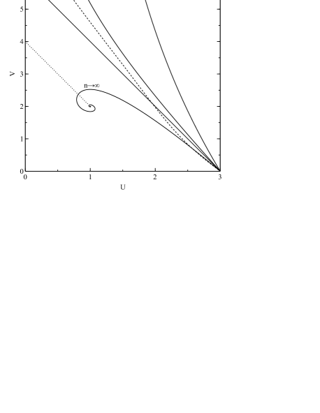
Figure 1: Some general features of the $U$–$V$ plane. The solid lines are, from top to bottom, polytropes of index $1$, $3$, $5$ and $\infty$. The dashed line is a stars model of a $1\hbox{$\,\text{M}_{\sun}$}$ star of solar metallicity when its radius is $1.012\hbox{$\,\text{R}_{\sun}$}$ and its luminosity $0.974\hbox{$\,L_{\sun}$}$. The dotted line shows the locus of the critical points $G_{s}$. The locus begins in the plane at $(0,4)$ when $n=3$ and tends to $(1,2)$ as $n$ increases to $\infty$.

Let us now return to the polytropic solutions for which we defined $U$ and $V$ in the first place. From the definitions above,

$$U=\frac{d\log\phi}{d\log\xi}=\frac{\xi^{3}\theta^{n}}{\phi}$$ (9)

and

$$V=-(n+1)\frac{d\log\theta}{d\log\xi}=(n+1)\frac{\phi}{\theta\xi}\text{.}$$ (10)

Let us differentiate $\log U$ and $\log V$ as they are defined for polytropes. This gives

$$\frac{1}{U}{\frac{\mathrm{d}U}{\mathrm{d}\xi}}=\frac{1}{\xi}[3-n(n+1)^{-1}V-U]$$ (11)

and

$$\frac{1}{V}{\frac{\mathrm{d}V}{\mathrm{d}\xi}}=\frac{1}{\xi}[-1+U+(n+1)^{-1}V]\text{.}$$ (12)

The ratio of these two equations yields the first-order equation

$${\frac{\mathrm{d}V}{\mathrm{d}U}}=-\frac{V}{U}\left(\frac{U+(n+1)^{-1}V-1}{U+n(n+1)^{-1}V-3}\right)$$ (13)

in which the dependence on $\xi$ has been eliminated. We refer to equation (13) as the homologous Lane–Emden equation (HLEE). The SC-like limits we wish to reproduce are shared by polytropic models so we now explore the behaviour of these solutions in the plane defined by $U$ and $V$.

2.3 Topology of the Homologous Lane–Emden Equation

The behaviour of solutions of the HLEE is described in terms of its critical points, where $dU/d\log\xi$ and $dV/d\log\xi$ both tend to zero. Horedt (1987) conducted a thorough survey of the behaviour of the HLEE, including the full range of $n$ from $-\infty$ to $\infty$ in linear, cylindrical and spherical geometries. Below, we use his convention for naming the critical points but consider only spherical cases with $n\geq 1$. Though realistic polytropes take $n$ in the range $3/2$ to infinity, we extend it to accommodate SC-like limits discussed in the literature for polytropic envelopes with $n=1$.

From the numerator of equation (13), we see that $dV/dU=0$ when $V=0$ or $U+V/(n+1)=1$. The former indicates that solutions that approach the $U$-axis proceed along it until they reach infinity or a critical point. The latter defines a straight line in the $U$–$V$ plane along which solutions are locally horizontal. Following Faulkner (2005) we refer to this line as the line of horizontals. Similarly, from the denominator, we find $dU/dV=0$ when $U=0$ or $U+nV/(n+1)=3$. Again, the first locus implies that solutions near the $V$-axis have trajectories that are nearly parallel to it, while the second gives another straight line, this time along which solutions are vertical, hereinafter referred to as the line of verticals. The critical points of the HLEE are located at the intersections of these curves. Below, we consider the stability of the critical points as $n$ varies. The analysis on which the discussion is based is provided in the Appendix.

The origin is the first critical point. It is a saddle with the solutions on the $V$-axis approaching and those on the $U$-axis escaping. Solutions near the origin move down and to the right on the $U$–$V$ plane. There is a further critical point on each of the axes. On the $U$-axis, $U_{s}=(3,0)$ is a saddle for all values of $n$. It is stable along the $U$-axis and unstable across it. This point coincides with the regular centre of realistic stellar models that we discussed previously. Along the $V$-axis, $V_{s}=(0,n+1)$ is also a critical point. For $n<3$ it is a source and for $n>3$ a saddle. The intersection of the lines of horizontals and verticals is the final critical point $G_{s}$. For each n, $G_{s}=(\frac{n-3}{n-1},2\frac{n+1}{n-1})$. The character of these points varies with $n$. Their locus is shown in Fig. 1.

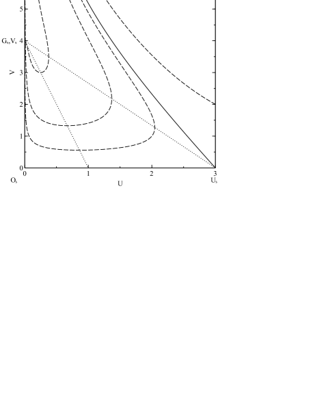
Figure 2: Topology of the HLEE for $n=3$. The solid line is the polytrope. The upper and lower dotted lines are the lines of verticals and horizontals, respectively. The dashed lines are a selection of solutions. Below the polytrope, the solutions have a non-zero mass at the centre, which is represented by the critical point $V_{s}=(0,4)$. Conversely, solutions above the polytrope have zero mass at non-zero inner radius.

The behaviour of $G_{s}$ and $V_{s}$ distinguishes the topology of solutions into three regimes. For $n<3$, $V_{s}$ is a pure source: it is unstable across and along the $V$-axis. The point $G_{s}$ has $U<0$ and therefore does not feature in the first quadrant of the $U$–$V$ plane but approaches the $V$-axis from the left as $n\to 3$. When $n=3$, $V_{s}$ and $G_{s}$ co-incide. The point is marginally stable across the axis. For $n>3$, $V_{s}$ and $G_{s}$ separate. $V_{s}$ is now a saddle and $G_{s}$ a source, gradually moving towards its position at $(1/2,3)$ when $n=5$. Fig. 2 illustrates some features of the HLEE when $n=3$. The lines of verticals and horizontals meet at $G_{s}$, which has just appeared on the $U$–$V$ plane at $(0,4)$.

Figure 3: Topology of the HLEE for $n=5$. The solid line is the polytrope. The dotted line from $V_{s}=(6,0)$ to $(1,0)$ is the line of horizontals. The other dotted line, from $(0,18/5)$ to $(3,0)$, is the line of verticals. The point $G_{s}=(1/2,3)$ is now distinct from $V_{s}$ and is a centre, as can be seen from the solutions, represented by the dashed lines. Below the polytrope, the solutions orbit $G_{s}$. Above, they extend from a finite inner radius, where $\phi=0$, to a finite outer mass and radius.

When $n=5$, which separates the cases of finite and infinite polytropes, the $U$–$V$ plane takes on a particular structure, illustrated in Fig. 3. The $n=5$ polytrope is a straight line from $U_{s}=(3,0)$ to $V_{s}=(0,6)$. The point $G_{s}$ is a centre, with solutions forming closed loops around it. The polytrope separates solutions that circulate around $G_{s}$ from those that go from $(\infty,0)$ to $(0,\infty)$ entirely above the polytrope. These solutions have zero mass at non-zero inner radius but, unlike the polytrope, have a finite outer radius.

As $n$ increases further $G_{s}$ becomes a spiral sink. Polytropes start at $U_{s}$ and now spiral into $G_{s}$ (see Fig. 1). There is an unstable solution that proceeds from $(\infty,0)$ to $V_{s}$ above which solutions extend to $(0,\infty)$. As $n\to\infty$ we also find $V_{s}\to(0,\infty)$ and, in the limiting case of the isothermal sphere, all solutions ultimately spiral into $G_{s}$ because they cannot lie above the unstable solution.

3 Fractional core mass contours

Let us consider the problem of fitting a polytropic envelope to a core of arbitrary mass and radius. For a given $n<5$, we can regard a given point $(U_{0},V_{0})$ in the $U$–$V$ plane as the interior boundary of a corresponding polytropic envelope by integrating the LEE from that point to the surface. More precisely, we can take interior conditions

$$\theta_{0}=1\text{,}$$ (14)

$$\xi_{0}=\sqrt{(n+1)^{-1}U_{0}V_{0}}\text{,}$$ (15)

and

$$\phi_{0}=\sqrt{(n+1)^{-3}U_{0}V_{0}^{3}}$$ (16)

and integrate the LEE up to the first zero of $\theta$ where we set $\xi=\xi_{1}$. This point marks the surface of a polytropic envelope, at which the dimensionless mass co-ordinate $\phi_{1}$ is the total mass of the solution, including the initial value $\phi_{0}$. The ratio $q=\phi_{0}/\phi_{1}$ is then the fractional mass of a core that occupies a dimensionless radius $\xi_{0}$. By associating each point in the $U$–$V$ plane with the value of $q$ for a polytropic envelope that starts there, we define a surface $q(U,V)$. We use the contours of this surface to characterise the SC limit.

Figs 4 and 5 show contours of $q(U,V)$ for polytropic envelopes with $n=3$ and $n=1$ respectively, along with a selection of interior solutions that lead to SC-like limits. For $n<3$ the contours are dominated by the critical point $V_{s}$ and for $n>3$ by $G_{s}$. Away from $V_{s}$ or $G_{s}$ all the contours at first curve away from the $U$-axis and then tend towards straight lines.

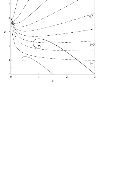
Figure 4: The dashed lines are contours of a core’s fractional mass $q=\phi_{0}/\phi_{1}$ beneath an envelope with $n=3$. They increase in steps of $0.1$ from $0.1$, at the bottom, to $0.9$, at the top. The larger solid spiral is the isothermal core with $\alpha=1$. The smaller spiral represents an isothermal core when $\alpha=2$. The upper and lower straight lines represent the inner boundaries for quasi-stars with $b=3$ and $b=1$ respectively (see Section 3.3).

3.1 The Schönberg–Chandrasekhar Limit

Kippenhahn & Weigert (1990) discuss the SC limit in terms of fractional mass contours. Cannon (1992) also explicitly described the SC limit in terms of fractional mass contours, although he employed a different set of homology-invariant variables. Fig. 4 shows the isothermal solution along with the fractional mass contours for $n=3$ envelopes. The SC limit exists because the isothermal solution only intersects fractional mass contours up to a maximum $q_{\text{max}}=0.359$ when $\alpha=1$. In other words, along the isothermal solution, the function $q(U,V)$ achieves a maximum of $0.359$.

A maximum $V$ for the isothermal curve exists because, for a given mass, there is a finite maximum pressure that a core can exert. This limit is usually derived by defining the core pressure using virial arguments and maximizing it with respect to the core radius (e.g. Kippenhahn & Weigert, 1990). Such an explanation partly describes the SC limit but our interpretation makes clear that the existence of the SC limit has as much to do with the behaviour of the envelope solutions as the isothermal core. For example, changing the polytropic index of the envelope changes the mass limit.

Figure 5: The dashed lines are contours of fractional mass $q=\phi_{0}/\phi_{1}$ for $n=1$. The solid spiral is again the isothermal core solution. The top-most diagonal line is the polytrope of index $5$ with $\alpha=1$. The other diagonal lines are, from top to bottom, core-envelope boundary conditions for the envelope when $\alpha=2,3,4$ for $n=5$ as shown by Eggleton et al. (1998, Fig. 3).

If there is a density jump by a factor $\alpha$ at the core-envelope boundary (see Section 2.2), then $U$ and $V$ at the edge of the core must be transformed to find the base of the envelope in the $U$–$V$ plane. That is, if $\rho\to\alpha^{-1}\rho$, then $(U,V)\to\alpha^{-1}(U,V)$. The contraction of the isothermal core for $\alpha=2$ is included in Fig. 4. The inner boundary of the envelope shifts to a smaller fractional mass of about $0.09$ so the SC limit falls too.

The argument presented here implies that SC-like limits exist whenever an envelope is matched to a core that only intersects fractional mass contours of that envelope up to some maximum. We now use this to explain the existence of other mass limits in the literature.

3.2 Related Polytropic Limits

Fig. 5 shows the fractional mass contours for $n=1$, the isothermal solution, and $n=5$ polytropes with $\alpha=1,2,3,4$ as used by Eggleton et al. (1998). Beech (1988) calculated an SC-like limit for an isothermal core embedded in a polytropic envelope with $n=1$. Because the behaviour of fractional mass contours is similar for $n=1$ and $n=3$, the existence of the limit is now no surprise. Note that the numerical value found by Beech (1988) differs because he included the radiation pressure of the isothermal core, which displaces $U$ and $V$ at the core-envelope boundary.

The conclusions of Eggleton et al. (1998) are also catered for. The critical point $V_{s}=(0,n+1)$ separates solutions, and thus contours, with $q\approx 0$ from those with $q\approx 1$. Eggleton et al. (1998) concluded that, for $n=1$ envelopes, cores with $n<5$ are never subject to an SC limit; those with $n>5$ always are; and those with $n=5$ constitute the marginal case for which the limit exists when $\alpha>3$. Eggleton et al. (1998) extended their arguments to changing the polytropic index of the envelope. Because these conclusions are based on the critical behaviour of the solutions, which is reflected in the behaviour of the contours, the same results follow here. We have shown how they are characterised by the contours in the same way as other limits and are a particular example of our broader result. That is, we have shown that SC-like limits exist whenever the core solution fails to intersect all fractional mass contours. The cases identified by Eggleton et al. (1998) fall within this description.

3.3 Loaded Polytropes and Quasi-stars

Quasi-stars are objects consisting of a stellar-mass black hole embedded in a massive, hydrostatic, giant-like envelope, potentially formed when primordial gas in large dark matter haloes collapsed in the early Universe (Begelman et al., 2006). The black hole is able to grow rapidly as long as the hydrostatic structure persists. Following the simple models described by Begelman, Rossi & Armitage (2008), Ball et al. (2011) computed models with the Cambridge stars code and found a maximum mass for the black hole that was accurately reproduced by polytropic models. We now show how this result is related to our analysis of the SC limit.

The interior boundary condition for the quasi-star models can be written as

$$r_{0}=\frac{1}{b}\frac{2Gm_{0}}{c_{s}^{2}}\text{,}$$ (17)

where $b$ is a scale factor, $m_{0}$ is the mass interior to $r_{0}$ and $c_{s}^{2}=\gamma p/\rho$ is the adiabatic sound speed. The boundary condition is then a fraction $1/b$ of the Bondi radius, where $mc_{s}^{2}/2=Gm/r$. Begelman et al. (2008) used $b=3$; Ball et al. (2011) used $b=1$. Accretion on to the central black hole supports the envelope by radiating near the Eddington limit of the entire object so the envelope is strongly convective and the pressure is dominated by radiation. The envelope is approximately polytropic with index $n=3$. Now, at the interior boundary, $c_{s}^{2}=(1+1/n)K\rho_{c}^{1/n}$, $m_{0}=4\pi\eta^{3}\rho_{c}\phi_{0}$, and $r_{0}=\eta\xi_{0}$ so

$$\phi_{0}=\frac{b}{2n}\xi_{0}\text{.}$$ (18)

Transforming to $U$ and $V$ gives $U_{0}=2n\xi_{0}^{2}/b$ and $V_{0}=b(n+1)/2n$. Varying $\xi_{0}$ traces a straight line, parallel to the $U$-axis. In Fig. 4, we have plotted $V_{0}=2/3$ and $2$, which correspond to $b=1$ and $3$, respectively, for $n=3$. The line of $V_{0}$ does not intersect all the contours of fractional core mass because many of them are positively curved. Thus, a mass limit exists, as in previous cases. For larger values of $b$, $V_{0}$ is also larger and intersects more of the contours. The mass limit is therefore larger.

We have limited ourselves to the case where $n=3$. The fractional mass contours in Figs 4 and 5 show similar behaviour. Convective envelopes are approximately adiabatic and have effective polytropic indices between $3/2$ and $3$, depending on the relative importance of gas and radiation pressures. All such envelopes possess fractional mass contours that are similar to the two cases here and we conclude that a fractional mass limit for the black hole exists in all realistic cases. Envelopes with $3<n<5$ have more complicated fractional mass contours so we cannot immediately draw similar conclusions.

This mass limit is not exactly the same as found by Ball et al. (2011). They computed the Bondi radius using the mass of the black hole only, even once the mass of gas inside the Bondi radius is comparable to (and even exceeds) the mass of the black hole. Begelman (2010, private communication) pointed out that the Bondi radius should be defined for the total mass inside $r_{0}$, not just the black hole mass. Presuming that the gas has a density distribution $\rho(r)\propto r^{-3/2}$ inside the cavity around the black hole, this gives the equation

$$r_{0}=\frac{2G}{c_{s}^{2}}\left(M_{\text{BH}}+\frac{8\pi}{3}\rho_{0}r_{0}^{3}\right)\text{,}$$ (19)

where $M_{\text{BH}}$ is the mass of the black hole only, for $b=1$. Making the same substitutions as in equation (18) for polytropic index $n=3$, the equation becomes

$$\phi_{\text{BH}}+\frac{2}{3}\xi_{0}^{3}-\frac{1}{6}\xi_{0}=0\text{,}$$ (20)

which only has a real positive root if $\phi_{\text{BH}}<1/(18\sqrt{3})$. The corresponding fractional core mass limit is $q=0.0166$.

In trying to move $r_{0}$ inwards, we found (Ball et al., 2011) we could not construct models with $b\geq 3.8$ in equation (17). We can see how this comes about from the behaviour of the polytropic limit. As $b$ increases, $V_{0}$ increases and eventually passes the critical point $G_{s}$ when the nature of the limit is reversed. When $b>2n$, small inner masses correspond to envelopes with negligible envelope mass so it becomes impossible to embed a small black hole inside a massive envelope. In other words, the mass limit becomes a minimum inner mass limit. For the models of Ball et al. (2011), the finite mass of the black hole corresponds to a finite value of $U_{0}$ that displaces the envelope slightly from the $V$-axis. The fractional mass contours are closely packed near $G_{s}$, so a small value of $U_{0}$ introduces a minimum inner mass limit for $b<2n$.

4 General Limits

The SC-like limits discussed above all exist because each locus of core-envelope boundaries only intersects fractional mass contours with $q$ smaller than some $q_{\text{max}}$. We can use this condition to identify large classes of core solutions that lead to SC-like limits. For example, an SC-like limit must exist whenever the core solution has everywhere $V<n_{\text{e}}+1$, where $n_{\text{e}}<5$ is the polytropic index of the envelope. Cores described by $n=5$ polytropes with $\alpha>6/(n_{\text{e}}+1)$, as discussed by Eggleton et al. (1998), satisfy this condition. SC-like limits also exist whenever the curve defining the inner edge of the envelope touches but does not cross some fractional mass contour. This explains the original SC limit and also implies that any composite polytrope with $n>5$ in the core and $n<5$ in the envelope is subject to an SC-like limit. In fact, the limits are determined by behaviour of solutions at the core-envelope boundary, so SC-like limits also exist when there is a layer with $n\gg 5$ at the base of the envelope. The constraint becomes even stronger as the density gradient at the core-envelope boundary becomes steeper or the mean molecular weight jump becomes more pronounced. Both of these conditions become relevant immediately after a star leaves its core-burning sequence, which implies that SC-like limits apply earlier in a star’s life than previously thought.

For a given core solution and polytropic index of the envelope, there are potentially two solutions either side of an SC-like limit that correspond to the same fractional core mass. The evolutionary sequence of static models determines which solutions occur in reality. For example, quasi-stars are initially constructed by loading a star with a small mass $q\ll 10^{-3}$. These lie close to the $V$-axis so solutions must start with $U_{0}\approx 0$ on the locus of inner boundary conditions and move towards greater $U_{0}$ as the black hole grows and the quasi-star evolves. The evolution halts when the maximum mass is achieved because the black hole cannot lose mass. Further solutions, with smaller inner masses than the maximum, exist as $U_{0}$ increases further. We have calculated polytropic models with $U_{0}$ greater than the SC-limited value but we were not able to compute STARS models along the same sequence.

It is also possible to test whether a given composite polytrope is at an SC-like limit. If the core solution touches but does not cross the contour corresponding to the given fractional core mass, then the model is at an SC-like limit. If this condition is satisfied, then extending or contracting the core can only admit a smaller fractional core mass. The test can be applied to realistic stellar models but identifying stars that have reached an SC-like limit is difficult. The inner edge of the envelope is not clearly defined and the effective polytropic index varies throughout the envelope.

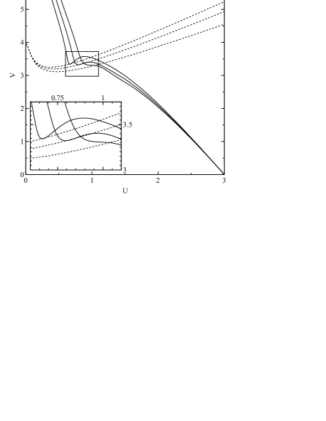
Figure 6: The solid lines are Cambridge stars models of a $1\hbox{$\,\text{M}_{\sun}$}$ pure helium star. Evolution proceeds from the right-most line at large $V$ to the left. The short-dashed lines are, from bottom to top, contours of fractional masses $0.516$, $0.543$ and $0.562$ for $n=3$. The inset is a magnification of the boxed region. The first model is at the end of the core He-burning sequence. The second model appears to have reached an SC-like limit of $q\approx 0.543$ according to our criterion. At this point, the star begins to expand rapidly and $T_{\text{eff}}$ decreases. As it evolves across the Hertzsprung gap, the gradient $\partial V/\partial U$ becomes steeper than the contours for the relevant fractional core mass.

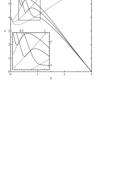
Figure 7: The solid lines are Cambridge stars models of a $0.5\hbox{$\,\text{M}_{\sun}$}$ pure helium star. Evolution proceeds from the right-most line at large $V$ to the left. The short-dashed lines are, from bottom to top, contours of fractional masses $0.640$, $0.740$ and $0.825$ for $n=3$. The inset is a magnification of the boxed region. The first model has already left the core He-burning sequence. The second model appears to be at an SC-like limit of $q_{\text{max}}\approx 0.74$ but, although the star is expanding, it does not evolve into a giant. The third model is at the maximum luminosity achieved by the model and is still at or near an SC-like limit. As the star continues to evolve, its profile in the $U$–$V$ plane tends to a polytrope with $n\approx 1.5$. The star does not become a giant and evolves directly on to the white-dwarf cooling sequence.

Despite the approximate nature of the test, we have applied it to models produced by the Cambridge stars code. Figs 6 and 7 show models of pure helium stars of $1\hbox{$\,\text{M}_{\sun}$}$ and $0.5\hbox{$\,\text{M}_{\sun}$}$. The envelopes are still mostly radiative and their effective polytropic indices vary between $n=2.5$ and $3.5$, so we have used fractional mass contours for envelopes with $n=3$ everywhere. The mass co-ordinate at the core-envelope boundary was determined approximately by eye at the point where $V$ was at a local minimum. Where a minimum did not exist a similar nearby point in the models was taken around where $\partial V/\partial U$ was a maximum. Based on these, both stars appear to reach SC-like limits shortly after moving off their core-burning sequences although their subsequent evolution is different (see Section 4.2). The regions which lie parallel to the contours have $n\gg 5$. Although the $n=3$ contours are an approximation, it appears that both stars reach SC-like limits shortly after leaving their core-burning sequence.

4.1 Beyond the limit

What happens when an isothermal core exceeds an SC-like limit? In short, its effective polytropic index must change. This can happen in two ways. Under suitable conditions, the inner part of the core becomes degenerate. Degenerate matter is described by a polytropic equation of state with $n=3$ or $n=3/2$ in relativistic and non-relativistic cases, respectively. The inner core can tend to such an equation with an isothermal layer further from the centre. An SC-like limit still exists but the isothermal layer is displaced upwards in $V$, so a larger core mass is possible. Alternatively, the core departs from thermal equilibrium and contracts. For an ideal gas, $dp/d\rho=1+1/n=1+dT/d\rho$, so the temperature gradient decreases the effective polytropic $n$. As long as $n\gg 5$, an SC-like limit persists but, as in the previous case, it corresponds to a larger fractional core mass.

The structure of the envelope offers some respite from the constraints imposed by the core. For radiative envelopes, where $n$ is not much greater than $3$, the fractional mass contours are much like those shown in Fig. 4. If the envelope becomes convective, then the effective polytropic index varies between $3/2$ and $3$. An SC-like limit still exists but the behaviour of the fractional mass contours is less extreme near $V_{s}$ for smaller values of $n$ (compare Figs 4 and 5). Away from $G_{s}$, contours run along smaller values of $V$ for smaller $n$. Equivalently, $q(U,V)$ is larger at a given point $(U,V)$ for small values of $n$. For example, for $n=3$, $q(2,4)=0.528$, whereas for $n=3/2$, $q(2,4)=0.562$ and for $n=1$, $q(2,4)=0.576$. Thus, a smaller polytropic index in the envelope permits a larger fractional core mass.

4.2 Evolution into giants

Although the evolution of main-sequence stars into giants is reproduced by detailed calculations of stellar structure, the cause of a star’s substantial expansion after leaving the main sequence remains unknown. Eggleton & Cannon (1991) showed that if the effective polytropic index of a star is everywhere less than some $n_{\text{max}}<5$, then it is less centrally condensed (i.e. $\rho_{c}/\bar{\rho}$ is smaller) than the polytrope of index $n_{\text{max}}$. Eggleton (2000) further conjectured that the evolution of dwarfs into giants during shell burning therefore requires that a significant part deep in the envelope has an effective polytropic index $n\gg 5$. This condition is similar to the condition under which a star is subject to an SC-like limit and the phenomena may be related.

Fig. 6 shows the evolution of a $1\hbox{$\,\text{M}_{\sun}$}$ helium star. After core He-burning is complete, the star briefly contracts and nuclear fusion continues in the portion of the core that was not convective during its burning phase. The star expands slightly before appearing to reach an SC-like limit. At this point, the expansion of the envelope accelerates and the effective temperature decreases, indicating that it has begun to evolve into a giant. The star continues to move across the Hertzsprung gap and the calculation is terminated when C-burning begins at the centre of the core. We also evaluated the evolution of solar metallicity stars with masses $1$, $3$, $5$, $7$ and $9\hbox{$\,\text{M}_{\sun}$}$ and found qualitatively similar behaviour. All appear to reach an SC-like limit at the end of the main sequence, before starting to cross the Hertzprung gap and evolving into giants.

Fig. 7 shows the evolution of a $0.5\hbox{$\,\text{M}_{\sun}$}$ helium star. The star appears to reach an SC-like limit in its shell-burning phase when the fractional core mass is about $0.74$. The star expands briefly but the $U$–$V$ profile tends back towards a polytrope thereafter. If the mean molecular weight gradient were steeper then an SC-like limit would apply earlier because the gradients of the contours are shallower at smaller $V$. However, the density jump between helium and metals is modest and allows a large core to develop before a limit applies. The star’s surface temperature does not decrease until it reaches the white dwarf cooling sequence. Thus, although this star appears to reach an SC-like limit, it does not become a giant.

Both these stars appear to reach SC-like limits but only one becomes a giant. What is the crucial difference between them? In the $0.5\hbox{$\,\text{M}_{\sun}$}$ star, the expansion around the limiting point reduces the effective polytropic index in the burning shells and the limit relaxes slightly. In the $1\hbox{$\,\text{M}_{\sun}$}$ star, the burning shell is thinner, hotter and deeper within the envelope. The shell responds less to the expansion. It appears that reaching the limit leads to expansion of the envelope but the response of the structure may then release the star from its SC-like limit as for the $0.5\hbox{$\,\text{M}_{\sun}$}$ star and not the $1\hbox{$\,\text{M}_{\sun}$}$.

Another difference between the two stars is that, following the limiting point, the core of $1\hbox{$\,\text{M}_{\sun}$}$ star extends beyond the SC-like limit. The gradient of the core profile becomes steeper than the fractional core-mass contour, unlike the $0.5\hbox{$\,\text{M}_{\sun}$}$ star where it is approximately equal and then becomes shallower. Such a structure is not limited because, by reducing the radial size of the limiting region in the $U$–$V$ plane, a larger fractional core mass can be accommodated but in order to reach this point it must have been limited before.

5 Conclusion

We have shown that SC-like limits exist whenever the solution describing a stellar core only intersects a fraction of contours of constant fractional mass for envelopes with a given polytropic index. Our description explains the original SC limit, SC-like limits found by Beech (1988) and Eggleton et al. (1998), and the limit for polytropic quasi-stars found by Ball et al. (2011). It also shows that SC-like limits exist under a wide range of circumstances. This includes models where the core solution touches but does not cross a particular fractional mass contour, as is the case if there is a layer with $n\gg 5$ at the base of the envelope.

We also derived a test of whether a polytropic model is at an SC-like limit. If the core solution touches but does not cross the contour of the appropriate fractional mass, then the model is SC-limited. Although the condition is only approximate for realistic models, we have applied it to helium stars and found that achieving a limit corresponds with expansion of their envelopes. Stars that clearly exceed an SC-like limit consistently evolve into giants but it is not known if this connection is causal. We have thus demonstrated that the original SC limit is a particular case of a broader phenomenon, that SC-like limits apply earlier in a star’s evolution than previously thought, and that there is a connection between exceeding these limits and evolving into a giant.

Appendix A:

From equations (11) and (12), we find

$${\frac{\mathrm{d}U}{\mathrm{d}\log\xi}}=-U[U+n(n+1)^{-1}V-3]$$ (21)

and

$${\frac{\mathrm{d}V}{\mathrm{d}\log\xi}}=V[U+(n+1)^{-1}V-1]\text{.}$$ (22)

This is an autonomous system of equations: the derivatives depend only on the dependent variables $U$ and $V$. The linear behaviour of such systems around the critical points can be characterised by the eigenvectors and eigenvalues of the Jacobian matrix (e.g. Strogatz, 1994),

$$J =\left(\begin{array}[]{cc}{\frac{\partial}{\partial U}}{\frac{\mathrm{d}U}{\mathrm{d}\log\xi}}&{\frac{\partial}{\partial V}}{\frac{\mathrm{d}U}{\mathrm{d}\log\xi}}\\ {\frac{\partial}{\partial U}}{\frac{\mathrm{d}V}{\mathrm{d}\log\xi}}&{\frac{\partial}{\partial V}}{\frac{\mathrm{d}V}{\mathrm{d}\log\xi}}\end{array}\right)$$ (25)

$$=\left(\begin{array}[]{c@{}c}3-2U-\frac{n}{n+1}V&-\frac{n}{n+1}U\\ \\ V&-1+U+\frac{2}{n+1}V\end{array}\right)\text{,}$$ (29)

at the critical point in question. In particular, if the real component of an eigenvalue is positive or negative, solutions tend away from or towards that point along the corresponding eigenvector. Such points are sources or sinks. When the point has one positive and one negative eigenvalue it is a saddle. If the eigenvalues have imaginary components then solutions orbit the point as they approach or recede. We describe these as spiral sources or sinks. If the eigenvalues are purely imaginary, then solutions form closed loops around that point, which we call a centre. The choice of independent variable, in this case $\log\xi$, is not relevant in such analysis.

Table 1 shows the eigenvalues and eigenvectors for the critical points in Section 2.3 as functions of $n$. The origin $O_{s}$ is always a saddle, with paths approaching along the $V$-axis and escaping along the $U$-axis. Because $n\geq 1$ for realistic or interesting models, $U_{s}$ also keeps the same saddle behaviour in our discussion, with points approaching along the axis and escaping along the other eigenvector, which always points towards the top left of the $U$–$V$ plane. For $n<3$, $V_{s}$ is a source. One eigenvector is always along the $V$-axis and the other across it but the latter varies from pointing up in the $U$–$V$ plane to pointing down. When $n=3$ one eigenvalue is zero so that it is a point of marginal stability. Points along the corresponding eigenvector are also stationary in the linear regime. As $n$ increases past $3$, $V_{s}$ becomes a saddle, with points now approaching from positive $U$.

Lastly, $G_{s}$ displays the most complicated behaviour. It first appears in the $U$–$V$ plane when $n=3$. In this case, it co-incides with $V_{s}$. As $n$ increases, $G_{s}$ is at first a source. When $\Delta_{n}=\sqrt{1+n(22-7n)}=0$, the eigenvalues take on an imaginary component, so $G_{s}$ becomes a spiral source. Increasing in $n$, the special case $n=5$ is reached. The eigenvalues become purely imaginary at $G_{s}$, so the point is a pure centre (see Fig. 3). For $n>5$, the real part of $G_{s}$ is negative and it becomes a spiral sink. As $n\to\infty$, $V_{s}$ effectively vanishes and all solutions ultimately reach $G_{s}$.

Table 1: Critical points of the HLEE. $\Delta_{n}=\sqrt{1+n(22-7n)}$.

Critical point		Eigenvalues		Eigenvectors
$O_{s}$	$(0,0)$	$3$	$-1$	$(1,0)$	$(0,1)$
$U_{s}$	$(3,0)$	$-3$	$2$	$(1,0)$	$(-3n,5+5n)$
$V_{s}$	$(0,n+1)$	$1$	$3-n$	$(0,1)$	$(2-n,1+n)$
$G_{s}$	$\left(\frac{n-3}{n-1},2\frac{n+1}{n-1}\right)$	$\frac{n-5\pm\Delta_{n}}{2-2n}$		$(1-n\mp\Delta_{n},4+4n)$

References

- Ball et al. (2011) Ball W. H., Tout C. A., Żytkow A. N., Eldridge J. J., 2011, MNRAS, 414, 2751
- Beech (1988) Beech M., 1988, Ap&SS, 147, 219
- Begelman et al. (2008) Begelman M. C., Rossi E. M., Armitage P. J., 2008, MNRAS, 387, 1649
- Begelman et al. (2006) Begelman M. C., Volonteri M., Rees M. J., 2006, MNRAS, 370, 289
- Cannon (1992) Cannon R. C., 1992, PhD thesis, University of Cambridge
- Chandrasekhar (1939) Chandrasekhar S., 1939, An Introduction to the Study of Stellar Structure. Univ. Chicago Press, Chicago
- Eggleton (2000) Eggleton P. P., 2000 Unsolved Problems in Stellar Evolution. Cambridge Univ. Press, Cambridge, p. 172
- Eggleton & Cannon (1991) Eggleton P. P., Cannon R. C., 1991, ApJ, 383, 757
- Eggleton et al. (1998) Eggleton P. P., Faulkner J., Cannon R. C., 1998, MNRAS, 298, 831
- Faulkner (2005) Faulkner J., 2005 The Scientific Legacy of Fred Hoyle. Cambridge Univ. Press, Cambridge, p. 149
- Horedt (1987) Horedt G. P., 1987, A&A, 177, 117
- Horedt (2004) Horedt G. P., ed. 2004, Astrophysics and Space Science Library Vol. 306 of Astrophysics and Space Science Library. Kluwer, Dordrecht
- Huntley & Saslaw (1975) Huntley J. M., Saslaw W. C., 1975, ApJ, 199, 328