Ghost Chaplygin scalar field model of dark energy

Abstract

We investigate the correspondence between the ghost and Chaplygin scalar field dark energy models in the framework of Einstein gravity. We consider a spatially non-flat FRW universe containing the interacting dark energy with dark matter. We reconstruct the potential and the dynamics for the Chaplygin scalar field model according to the evolutionary behavior of the ghost dark energy which can describe the phantomic accelerated expansion of the universe.

PACS numbers: 98.80.-k, 95.36.+x
Keywords: Cosmology, Dark energy

1 Introduction

Observational data of type Ia supernovae (SNeIa) collected by Riess et al. [1] in the High-redshift Supernova Search Team and by Perlmutter et al. [2] in the Supernova Cosmology Project Team independently reported that the present observable universe is undergoing an accelerated expansion phase. The exotic source for this cosmic acceleration is generally dubbed “dark energy” (DE). Despite many years of research (see e.g., the reviews [3, 4]) its origin has not been identified till yet. DE is distinguished from ordinary matter (such as baryons and radiation), in the sense that it has negative pressure. This negative pressure leads to the accelerated expansion of the universe by counteracting the gravitational force. The astrophysical observations show that about 73% of the present energy of the universe is contained in DE. There are several DE models to explain cosmic acceleration.

One of interesting DE candidates is the Chaplygin gas which was proposed to explain the accelerated expansion of the universe [5]. The Chaplygin gas behaves as a pressureless dark matter (DM) at early times and like a cosmological constant at late stage [5]. This interesting feature leads to the Chaplygin gas model being proposed as a candidate for the unified DM-DE (UDME) scenario [6].

More recently, a new DE model called ghost DE (GDE) has been motivated from the Veneziano ghost of choromodynamics (QCD). The advantages of the GDE with respect to other DE models include the absence of the fine tuning and cosmic coincidence problems and the fact that it can be completely explained within the standard model and general relativity, without recourse to any new field, new degree(s) of freedom, new symmetries or modifications of general relativity [7]. Several aspects of this new paradigm, in particular observational constraints on this model, have been investigated in the literature [8].

The other interesting issue in modern cosmology is reconstructing the scalar field models of DE which has been investigated in the literature [9]. The scalar field models (such as quintessence, phantom, quintom, tachyon, K-essence, dilaton and Chaplygin) are often regarded as an effective description of an underlying theory of DE [10]. The scalar field models can alleviate the fine tuning and coincidence problems [11]. Scalar fields naturally arise in particle physics including supersymmetric field theories and string/M theory. Therefore, scalar field is expected to reveal the dynamical mechanism and the nature of DE. However, although fundamental theories such as string/M theory do provide a number of possible candidates for scalar fields, they do not uniquely predict its potential $V(\phi)$ [10]. Therefore it becomes meaningful to reconstruct $V(\phi)$ from some DE models (such as holographic, agegraphic and ghost).

All mentioned in above motivate us to investigate the correspondence between the GDE and the Chaplygin scalar field model of DE. To do so in Section 2, we study the interacting GDE with DM in a spatially non-flat Friedmann-Robertson-Walker (FRW) universe. In Section 3, we investigate the Chaplygin scalar filed model of DE. In Section 4, we suggest a correspondence between the interacting GDE and the Chaplygin scalar field model of DE. We reconstruct the potential and the dynamics for the ghost Chaplygin scalar field model. Section 5 is devoted to conclusions.

2 Interacting GDE with DM

The GDE density is given by [7]

$$\rho_{\Lambda}=\alpha H,$$ (1)

where $\alpha$ is a constant with dimension $[{\rm energy}]^{3}$, and roughly of order of $\Lambda_{\rm QCD}^{3}$ where $\Lambda_{\rm QCD}\sim 100$ MeV is QCD mass scale. With $H\sim 10^{-33}$ eV, $\Lambda^{3}_{\rm QCD}H$ gives the right order of observed DE density. This numerical coincidence is impressive and also means that this model gets rid of fine tuning problem [7].

Here, we investigate the GDE model in the framework of Einstein gravity. To do so, we consider a spatially non-flat FRW universe containing the GDE and DM. The first Friedmann equation in the standard FRW cosmology is

$$H^{2}+\frac{k}{a^{2}}=\frac{1}{3M_{\rm p}^{2}}(\rho_{\rm m}+\rho_{\Lambda}),$$ (2)

where $M_{\rm p}=(8\pi G)^{-1/2}$ is the reduced Planck mass and $H=\dot{a}/a$ is the Hubble parameter. Here, $k=0,1,-1$ represent a flat, closed and open FRW universe, respectively. Also $\rho_{\rm m}$ and $\rho_{\Lambda}$ are the energy densities of DM and GDE, respectively.

Using the usual definitions for the dimensionless energy densities as

$$\Omega_{\rm m}=\frac{\rho_{\rm m}}{\rho_{\rm cr}}=\frac{\rho_{\rm m}}{3M_{\rm p}^{2}H^{2}},~{}~{}~{}\Omega_{\Lambda}=\frac{\rho_{\Lambda}}{\rho_{\rm cr}}=\frac{\rho_{\Lambda}}{3M_{\rm p}^{2}H^{2}},~{}~{}~{}\Omega_{k}=\frac{k}{a^{2}H^{2}},$$ (3)

the Friedmann equation (2) can be rewritten as

$$1+\Omega_{k}=\Omega_{\rm m}+\Omega_{\Lambda}.$$ (4)

Substituting Eq. (1) into $\rho_{\Lambda}=3M_{\rm p}^{2}H^{2}\Omega_{\Lambda}$ yields

$$\Omega_{\Lambda}=\frac{\alpha}{3M_{\rm p}^{2}H}.$$ (5)

Using the above relation, the curvature energy density parameter can be obtained as

$$\Omega_{k}=\left(\frac{9M_{\rm p}^{4}k}{\alpha^{2}}\right)\frac{\Omega_{\Lambda}^{2}}{a^{2}}=\left(\frac{\Omega_{k_{0}}}{\Omega_{\Lambda_{0}}^{2}}\right)\frac{\Omega_{\Lambda}^{2}}{a^{2}},$$ (6)

where we take $a_{0}=1$ for the present value of the scale factor.

We further assume there is an interaction between GDE and DM. The recent observational evidence provided by the galaxy cluster Abell A586 supports the interaction between DE and DM [12]. In the presence of interaction, $\rho_{\Lambda}$ and $\rho_{\rm m}$ do not conserve separately and the energy conservation equations for GDE and pressureless DM are

$$\dot{\rho}_{\Lambda}+3H(1+\omega_{\Lambda})\rho_{\Lambda}=-Q,$$ (7)

$$\dot{\rho}_{\rm m}+3H\rho_{\rm m}=Q,$$ (8)

where $\omega_{\Lambda}=p_{\Lambda}/\rho_{\Lambda}$ is the equation of state (EoS) parameter of the interacting GDE and $Q$ stands for the interaction term. Following [13], we shall assume $Q=3b^{2}H\rho_{\Lambda}$ with the coupling constant $b^{2}$. This expression for the interaction term was first introduced in the study of the suitable coupling between a quintessence scalar field and a pressureless DM field [14, 15].

Taking time derivative of Eq. (1) and using (2), (4), (5) and (8) gives

$$\frac{\dot{\rho_{\Lambda}}}{\rho_{\Lambda}}=-\frac{3H}{2-\Omega_{\Lambda}}\left[1+\frac{\Omega_{k}}{3}-(1+b^{2})\Omega_{\Lambda}\right].$$ (9)

Taking time derivative of Eq. (5) and using (1) and (9) one can obtain the evolution of the GDE density parameter as

$$\frac{\Omega_{\Lambda}^{\prime}}{\Omega_{\Lambda}}=\frac{3}{2-\Omega_{\Lambda}}\left[1+\frac{\Omega_{k}}{3}-(1+b^{2})\Omega_{\Lambda}\right],$$ (10)

where $\Omega_{\Lambda}^{\prime}=\frac{{\rm d}\Omega_{\Lambda}}{{\rm d}\ln a}=\dot{\Omega}_{\Lambda}/H$. Using Eq. (6) and taking $\Omega_{k_{0}}=0.0125$ [16] for the present time, one can obtain $\Omega_{\Lambda}(a)$ by solving the differential equation (10) numerically with the initial condition $\Omega_{\Lambda_{0}}=0.725$ [16]. The numerical results obtained for $\Omega_{\Lambda}(a)$ are displayed in Fig. 1 for different coupling constants $b^{2}$. Figure 1 shows that: i) for a given $b^{2}$, $\Omega_{\Lambda}$ increases when the scale factor increases. ii) At early and late times, $\Omega_{\Lambda}$ increases and decreases with increasing $b^{2}$, respectively.

With the help of Eqs. (7) and (9), the EoS parameter of the interacting GDE can be obtained as

$$\omega_{\Lambda}=-\frac{1}{2-\Omega_{\Lambda}}\left(1-\frac{\Omega_{k}}{3}+2b^{2}\right).$$ (11)

Equation (11) shows that in the absence of interaction, i.e. $b^{2}=0$, at late times where $\Omega_{\Lambda}\rightarrow 1$ and $\Omega_{k}\rightarrow 0$, we have $\omega_{\Lambda}=-1$ which behaves like $\Lambda$CDM. Besides, taking $\Omega_{\Lambda_{0}}=0.725$ and $\Omega_{k_{0}}=0.0125$ for the present time then we obtain $\omega_{\Lambda_{0}}=-0.78$ which acts like the quintessence DE ($\omega_{\Lambda}>-1$). But in the presence of interaction, taking again $\Omega_{\Lambda_{0}}=0.725$ and $\Omega_{k_{0}}=0.0125$ for the present time then from Eq. (11) the EoS parameter can behave like phantom DE ($\omega_{\Lambda}<-1$) provided $b^{2}>0.14$. This value for the coupling constant $b^{2}$ is consistent with the observations [17]. Also the phantom divide crossing is compatible with the recent observations [16].

The evolution of the EoS parameter, Eq. (11), for different $b^{2}$ is plotted in Fig. 2. It shows that: i) for $b^{2}=0$, $\omega_{\Lambda}$ varies from $\omega_{\Lambda}>-1$ to $\omega_{\Lambda}=-1$, which is similar to the freezing quintessence model [18]. ii) For $b^{2}\neq 0$, $\omega_{\Lambda}$ varies from the quintessence phase ($\omega_{\Lambda}>-1$) to the phantom regime ($\omega_{\Lambda}<-1$). iii) For a given scale factor, $\omega_{\Lambda}$ decreases with increasing $b^{2}$.

For completeness, we give the deceleration parameter

$$q=-1-\frac{\dot{H}}{H^{2}},$$ (12)

which combined with the dimensionless density parameter $\Omega_{\Lambda}$ and the EoS parameter $\omega_{\Lambda}$ form a set of useful parameters for the description of the astrophysical observations. Using Eqs. (1), (9) and (12) one can get

$$q=\frac{1+\Omega_{k}-(2+3b^{2})\Omega_{\Lambda}}{2-\Omega_{\Lambda}}.$$ (13)

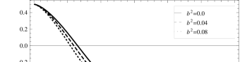
Figure 3: The deceleration parameter, Eq. (13), versus scale factor. Legend and auxiliary parameters as in Fig. 1.

In Fig. 3 we plot the evolutionary behavior of the deceleration parameter, Eq. (13), for different $b^{2}$. Figure 3 presents that: i) the universe transitions from a matter dominated epoch at early times to the de Sitter phase, i.e. $q=-1$, in the future, as expected. For $b^{2}=0.0$, $0.04$ and $0.08$ at $a=0.65$, $0.60$ and $0.54$, respectively, we have a cosmic deceleration $q>0$ to acceleration $q<0$ transition which is compatible with the observations [19]. ii) For a given scale factor, $q$ decreases with increasing $b^{2}$.

3 Interacting Chaplygin scalar field with DM

The EoS of the Chaplygin gas model of DE is as follows [5]

$$p_{\rm Ch}=-\frac{A}{\rho_{\rm Ch}},$$ (14)

where $A$ is a positive constant. Inserting the above EoS into the energy equation (7) leads to a density evolving as

$$\rho_{\rm Ch}=\frac{1}{\sqrt{1+b^{2}}}\left(A+\frac{B}{a^{6(1+b^{2})}}\right)^{1/2},$$ (15)

where $B$ is a positive integration constant. Note that the Chaplygin gas model in the absence of interaction term, i.e. $b^{2}=0$, offers a unified picture of DM and DE [6]. Because it smoothly interpolates between a non-relativistic matter phase ($\rho_{\rm Ch}\propto a^{-3}$) in the past and a negative-pressure DE regime ($\rho_{\rm Ch}=-p_{\rm Ch}$) at late times.

Using Eqs. (14) and (15) the EoS parameter of the interacting Chaplygin gas DE is obtained as

$$\omega_{\rm Ch}=\frac{p_{\rm Ch}}{\rho_{\rm Ch}}=-1-\frac{Ab^{2}-Ba^{-6(1+b^{2})}}{A+Ba^{-6(1+b^{2})}},$$ (16)

which shows that for $Ab^{2}>Ba^{-6(1+b^{2})}$ we have $\omega_{\rm Ch}<-1$ which corresponds to a universe dominated by phantom DE. In other words, crossing the phantom divide line occurs when

$$a>a_{\rm min}=\left(\frac{B}{Ab^{2}}\right)^{\frac{1}{6(1+b^{2})}}.$$ (17)

Note that in the absence of interaction ($b^{2}=0$), Eq. (16) gives $\omega_{\rm Ch}>-1$ which corresponds to a universe dominated by quintessence DE.

Here, one can obtain a corresponding potential for the Chaplygin gas DE by treating it as an ordinary scalar field $\phi$. Using Eqs. (14) and (15) together with $\rho_{\rm Ch}=\frac{1}{2}\dot{\phi}^{2}+V(\phi)$ and $p_{\rm Ch}=\frac{1}{2}\dot{\phi}^{2}-V(\phi)$, we find

$$\dot{\phi}^{2}=-\frac{Ab^{2}-Ba^{-6(1+b^{2})}}{(1+b^{2})^{\frac{1}{2}}\Big{[}A+Ba^{-6(1+b^{2})}\Big{]}^{\frac{1}{2}}},$$ (18)

$$V(\phi)=\frac{A(2+b^{2})+Ba^{-6(1+b^{2})}}{2(1+b^{2})^{\frac{1}{2}}\Big{[}A+Ba^{-6(1+b^{2})}\Big{]}^{\frac{1}{2}}}.$$ (19)

Equation (18) clears that for $Ab^{2}>Ba^{-6(1+b^{2})}$, the Chaplygin gas DE behaves like a phantom scalar filed, i.e. $\dot{\phi}^{2}<0$, whereas in the absence of interaction it acts like a quintessence scalar field ($\dot{\phi^{2}}>0$).

4 Correspondence between GDE and Chaplygin gas

Here, our aim is to investigate whether a minimally coupled Chaplygin scalar field can mimic the dynamics of the GDE model so that this model can be related to some fundamental theory (such as string/M theory), as it is for a scalar field. For this task, it is then meaningful to reconstruct the $V(\phi)$ of Chaplygin scalar field model possessing some significant features of the underlying theory of DE, such as the GDE model. In order to do that, we establish a correspondence between the GDE and Chaplygin gas scalar field by identifying their respective energy densities and equations of state and then reconstruct the potential and the dynamics of the field.

Equating Eqs. (1) and (15), i.e. $\rho_{\Lambda}=\rho_{\rm Ch}$, gives

$$A=\alpha^{2}H^{2}(1+b^{2})-Ba^{-6(1+b^{2})}.$$ (20)

Also equating Eqs. (11) and (16), i.e. $\omega_{\Lambda}=\omega_{\rm Ch}$, and using (20) we obtain

$$A=\frac{\alpha^{2}H^{2}}{2-\Omega_{\Lambda}}\left(1-\frac{\Omega_{k}}{3}+2b^{2}\right).$$ (21)

Substituting Eq. (21) into (20) yields

$$B=\alpha^{2}H^{2}a^{6(1+b^{2})}\left[1+b^{2}-\frac{1}{2-\Omega_{\Lambda}}\left(1-\frac{\Omega_{k}}{3}+2b^{2}\right)\right].$$ (22)

With the help of Eqs. (21) and (22) and using (5) one can rewrite (18) and (19) as

$$\dot{\phi^{2}}=\frac{\alpha^{2}}{3M_{\rm p}^{2}\Omega_{\Lambda}}\left[1-\frac{1}{2-\Omega_{\Lambda}}\left(1-\frac{\Omega_{k}}{3}+2b^{2}\right)\right],$$ (23)

$$V(\phi)=\frac{\alpha^{2}}{6M_{\rm p}^{2}\Omega_{\Lambda}}\left[1+\frac{1}{2-\Omega_{\Lambda}}\left(1-\frac{\Omega_{k}}{3}+2b^{2}\right)\right].$$ (24)

At the present time, if one takes $\Omega_{\Lambda}=0.73$ and $\Omega_{k}=0.01$ then from Eq. (23) one can obtain a phantom scalar field ($\dot{\phi}^{2}<0$) provided $b^{2}>0.14$.

From definition $\dot{\phi}=\phi^{\prime}H$ one can rewrite Eq. (23) as

$$\phi^{\prime}=\sqrt{3}M_{\rm p}\left\{\Omega_{\Lambda}\left[1-\frac{1}{2-\Omega_{\Lambda}}\left(1-\frac{\Omega_{k}}{3}+2b^{2}\right)\right]\right\}^{\frac{1}{2}},$$ (25)

where $\phi^{\prime}=\frac{{\rm d}\phi}{{\rm d}\ln a}$.

Using Eqs. (1) and (3), the evolutionary form of the Chaplygin gas scalar field can be obtained as

$$\phi(a)-\phi(a_{0})=\sqrt{3}M_{\rm p}\int^{a}_{a_{0}}\left[\frac{\Omega_{\Lambda}}{2-\Omega_{\Lambda}}\left(1-\Omega_{\Lambda}+\frac{\Omega_{k}}{3}-2b^{2}\right)\right]^{1/2}~{}\frac{{\rm d}a}{a}.$$ (26)

4.1 Numerical results

The integral (26) cannot be taken analytically. But with the help of Eq. (6) and numerical solution of the differential equation (10) one can take the integral (26), numerically. As we already mentioned, to solve Eq. (10) we need an initial condition for $\Omega_{\Lambda}$ where we take its present value at $a_{0}=1$. Besides, according to Eq. (6) we need the present value of $\Omega_{k_{0}}$. More recently, according to the 7-year WMAP data [16] the latest observational values of the aforementioned parameters have been reported as $\Omega_{\Lambda_{0}}=0.725\pm 0.016$ and $\Omega_{k_{0}}=-0.0125_{-0.0067}^{+0.0064}$ at 68% confidence level. Note that in [16] the curvature energy density parameter is defined as $\Omega_{k}=-\frac{k}{a^{2}H^{2}}$ which differs from our definition (3) by a minus sign. Here, we set the initial conditions to be the best fit values of $\Omega_{\Lambda_{0}}=0.725$ and $\Omega_{k_{0}}=0.0125$. Also we take $\phi(a_{0})=0$ at present time ($a_{0}=1$). The evolution of the Chaplygin gas scalar field (26) is plotted in Fig. 4. It shows that the Chaplygin scalar field increases when the scale factor increases. Figure 4 also clears that for a given scale factor, the Chaplygin scalar field decreases with increasing the coupling constant $b^{2}$. Note that in Fig. 4 for $b^{2}=0.04$ and $0.08$ at $a>2.13$ and $1.50$, respectively, $\phi$ becomes pure imaginary, i.e. $\dot{\phi}^{2}<0$, and does not show itself in Fig. 4. For $\dot{\phi}^{2}<0$ the Chaplygin scalar field behaves like phantom DE [20]. Note that when the phantom scalar fields give rise to constant EoS parameter $\omega_{\Lambda}$ smaller than $-1$, then the universe reaches a Big Rip singularity in the future [21]. In our model according to Fig. 2, for $b^{2}=0.0$, $0.04$ and $0.08$ when $a\rightarrow\infty$ we obtain $\omega_{\Lambda}=-1$, $-1.04$ and $-1.08$, respectively. This shows that in the presence of interaction for $a\rightarrow\infty$ we have the constant EoS parameter $\omega_{\Lambda}=p_{\Lambda}/\rho_{\Lambda}\simeq-1-b^{2}<-1$ and fate of the universe goes toward a Big Rip.

The variation of the Chaplygin scalar potential (24) versus the scalar field $\phi$ is plotted in Fig. 5. It shows that the Chaplygin scalar potential decreases when the scalar field increases. Figure 5 also presents that for a given scalar field, the Chaplygin scalar potential increases with increasing the coupling constant $b^{2}$.

5 Conclusions

Here we investigated the ghost Chaplygin scalar field model of DE in the framework of FRW cosmology. We considered a spatially non-flat FRW universe filled with the interacting GDE and pressureless DM. We derived a differential equation governing the evolution of the GDE density parameter. We also obtained the EoS parameter of the interacting GDE and the deceleration parameter. Furthermore, we established a correspondence between the GDE and the Chaplygin gas scalar field model. We reconstructed the dynamics and the potential of the Chaplygin gas scalar field according the evolutionary behavior of the GDE model which can describe the phantomic accelerated expansion of the universe at the present time. Our numerical results show the following.

(i) The interacting GDE density parameter $\Omega_{\Lambda}$ for a given coupling constant $b^{2}$, increases during history of the universe. Also at early and late times, $\Omega_{\Lambda}$ increases and decreases, respectively, with increasing $b^{2}$.

(ii) The EoS parameter $\omega_{\Lambda}$ of the GDE model can cross the phantom divide line ($\omega_{\Lambda}<-1$) at the present provided $b^{2}>0.14$ which is compatible with the observations. For $b^{2}=0$, $\omega_{\Lambda}$ behaves like the freezing quintessence DE. Also for $b^{2}\neq 0$, $\omega_{\Lambda}$ varies from the quintessence epoch ($\omega_{\Lambda}>-1$) to the phantom era.

(iii) The evolution of the deceleration parameter $q$ shows that the universe transitions from an early matter dominant phase to the de Sitter phase in the future which is in accordance with the observations.

(iv) The ghost Chaplygin scalar filed $\phi$ for a given $b^{2}$, increases with increasing the scale factor. Also for a given scale factor, it decreases with increasing $b^{2}$. The ghost Chaplygin potential $V(\phi)$ for a given $b^{2}$, decreases with increasing the scalar filed. For a given scalar field, $V(\phi)$ increases with increasing $b^{2}$.

Figure 1: The GDE density parameter, Eq. (10), versus scale factor for different coupling constants $b^{2}=$ 0 (solid line), 0.04 (dashed line) and 0.08 (dotted line). Auxiliary parameters are $\Omega_{\Lambda_{0}}=0.725$ and $\Omega_{k_{0}}=0.0125$ [16].

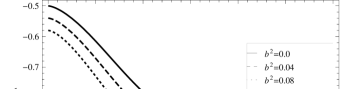
Figure 2: The EoS parameter of GDE, Eq. (11), versus scale factor. Legend and auxiliary parameters as in Fig. 1.

Figure 4: The Chaplygin gas scalar field, Eq. (26), versus scale factor. Legend and auxiliary parameters as in Fig. 1. Here $\phi(1)=0.0$.

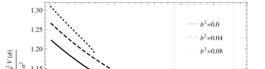
Figure 5: The Chaplygin gas scalar potential, Eq. (24), versus scalar field. Legend and auxiliary parameters as in Fig. 1.

References

- [1] A.G. Riess, et al., Astron. J. 116, 1009 (1998).
- [2] S. Perlmutter, et al., Astrophys. J. 517, 565 (1999).
-
[3]
T. Padmanabhan, Phys. Rep. 380, 235 (2003);
P.J.E. Peebles, B. Ratra, Rev. Mod. Phys. 75, 559 (2003). - [4] E.J. Copeland, M. Sami, S. Tsujikawa, Int. J. Mod. Phys. D 15, 1753 (2006).
-
[5]
A. Kamenshchik, U. Moschella, V. Pasquier, Phys. Lett. B 487,
7 (2000);
A. Kamenshchik, U. Moschella, V. Pasquier, Phys. Lett. B 511, 265 (2001);
N. Bilic, G.B. Tupper, R.D. Viollier, Phys. Lett. B 535, 17 (2002). -
[6]
P. Wu, H. Yu, Astrophys. J. 658, 663 (2007);
J. Lu, Y. Gui, L.X. Xu, Eur. Phys. J. C 63, 349 (2009). -
[7]
F.R. Urban, A.R. Zhitnitsky, Phys. Rev. D 80, 063001 (2009);
F.R. Urban, A.R. Zhitnitsky, JCAP 09, 018 (2009);
F.R. Urban, A.R. Zhitnitsky, Phys. Lett. B 688, 9 (2010);
F.R. Urban, A.R. Zhitnitsky, Nucl. Phys. B 835, 135 (2010);
N. Ohta, Phys. Lett. B 695, 41 (2011);
R.G. Cai, et al., Phys. Rev. D 84, 123501 (2011);
R.G. Cai, et al., Phys. Rev. D 86, 023511 (2012). -
[8]
E. Ebrahimi, A. Sheykhi, Phys. Lett. B 705, 19
(2011);
E. Ebrahimi, A. Sheykhi, Int. J. Mod. Phys. D 20, 2369 (2011);
A. Sheykhi, A. Bagheri, Europhys. Lett. 95, 39001 (2011);
A. Sheykhi, M. Sadegh Movahed, Gen. Relativ. Gravit. 44, 449 (2012);
A. Rozas-Fernandez, Phys. Lett. B 709, 313 (2012);
K. Saaidi, A. Aghamohammadi, B. Sabet, arXiv:1203.4518. -
[9]
X. Zhang, Phys. Rev. D 74, 103505
(2006);
J. Zhang, X. Zhang, H. Liu, Phys. Lett. B 651, 84 (2007);
K. Karami, J. Fehri, Phys. Lett. B 684, 61 (2010);
K. Karami, et al., Phys. Lett. B 686, 216 (2010). - [10] J.P. Wu, D.Z. Ma, Y. Ling, Phys. Lett. B 663, 152 (2008).
- [11] A. Ali, M. Sami, A.A. Sen, Phys. Rev. D 79, 123501, (2009).
- [12] O. Bertolami, F. Gil Pedro, M. Le Delliou, Phys. Lett. B 654, 165 (2007).
- [13] D. Pavón, W. Zimdahl, Phys. Lett. B 628, 206 (2005).
-
[14]
W. Zimdahl, D. Pavón, Phys. Lett. B 521, 133 (2001);
W. Zimdahl, D. Pavón, Gen. Relativ. Gravit. 35, 413 (2003);
L.P. Chimento, et al., Phys. Rev. D 67, 083513 (2003). -
[15]
L. Amendola, Phys. Rev. D 60, 043501 (1999);
L. Amendola, Phys. Rev. D 62, 043511 (2000);
L. Amendola, D. Tocchini-Valentini, Phys. Rev. D 64, 043509 (2001);
L. Amendola, C. Quercellini, Phys. Rev. D 68, 023514 (2003). - [16] E. Komatsu, et al., Astrophys. J. Suppl. 192, 18 (2011).
-
[17]
B. Wang, Y. Gong, E. Abdalla, Phys. Lett. B 624, 141
(2005);
B. Wang, C.Y. Lin, E. Abdalla, Phys. Lett. B 637, 357 (2005). - [18] R.R. Caldwell, E.V. Linder, Phys. Rev. Lett. 95, 141301 (2005).
- [19] E.E.O. Ishida, et al., Astropart. Phys. 28, 547 (2008).
- [20] R.R. Caldwell, Phys. Lett. B 545, 23 (2002).
-
[21]
J.V. Narlikar, T. Padmanabhan, Phys. Rev. D 32, 1928
(1985);
S.M. Carroll, M. Hoffman, M. Trodden, Phys. Rev. D 68, 023509 (2003);
P. Singh, M. Sami, N. Dadhich, Phys. Rev. D 68, 023522 (2003).