UNIVERSITY OF SOUTHAMPTON
FACULTY OF PHYSICAL AND APPLIED SCIENCES
School of Physics and Astronomy
Southampton High Energy Physics Group
Phenomenological Aspects
of the $E_{6}$SSM
by
Jonathan Peter Hall
Presented for the degree of
Doctor of Philosophy
November 2011

The work in this thesis explores various phenomenological aspects of the $E_{6}$SSM with a particular focus on the inert neutralino sector of the model and on the dark matter implications. The $E_{6}$SSM is a string theory inspired supersymmetric extension to the Standard Model with an $E_{6}$ grand unification group. The model provides a solution to the hierarchy problem of the Standard Model, provides an explanation for neutrino mass, and has automatic gauge anomaly cancellation.

The inert neutralino sector of the $E_{6}$SSM and the dark matter that naturally arises from this sector is studied for the first time. Limits on the parameter space from experimental and cosmological observations relating to the inert neutralino dark matter are explored and the consequences for Higgs boson phenomenology are investigated. In plausible scenarios it is found that the couplings of the lightest inert neutralinos to the SM-like Higgs boson are always rather large. This has major implications for Higgs boson collider phenomenology and leads to large spin-independent LSP-nucleon cross-sections. Because of the latter, scenarios in which $E_{6}$SSM inert neutralinos account for all of the observed dark matter are now severely challenged by recent dark matter direct detection experiment analyses. In plausible scenarios consistent with observations from both cosmology and LEP the lightest inert neutralino is required to have a mass around half of the $Z$ boson mass if it contributes to cold dark matter and this means that $\tan(\beta)$ cannot be too large.

A new variant of the $E_{6}$SSM called the $E_{6}\mathds{Z}^{S}_{2}$SSM is also presented in which the dark matter scenario is very different to the inert neutralino cold dark matter scenario and in which the presence of supersymmetric massless states in the early universe modifies the expansion rate of the universe prior to Big Bang Nucleosynthesis. The new dark matter scenario is consistent with current observations and the modified expansion rate provides a better explanation of various data than the SM prediction. The prospects for a warm dark matter scenario in the $E_{6}$SSM are also briefly discussed.

 

Dedicated to my friends and family
and to those whom we have lost.

Author’s Declaration

I declare that this thesis has been composed by myself and constitutes work completed by myself wholly while I was in candidature for a research degree at the University of Southampton. Where the published work of others has been consulted or quoted from this is always clearly attributed and all main sources of help have been acknowledged.
I make no claim of originality for the work in chapters 1–4 and appendices A and B. These chapters present background information compiled from a variety of sources that have been referenced in the text. Chapter 5 contains work that was previously published in paper I. This work was carried by myself out under the supervision of my Ph.D. supervisor Steve King. Chapter 6 contains work that was previously published in paper II. This work was a collaborative effort between the authors. I was directly responsible for the calculation of the dark matter relic density using micrOMEGAs and for the generation of the benchmark points in tables 6.1 and 6.2 and of the plots in figure 6.1 and directly worked on the RG and direct detection analyses. Chapter 7 contains work that was previously published in paper III with the exception of section 7.5 which contains work that is original to this thesis. This work was carried out by myself under the supervision of Steve King.

Signed:

Date:

Paper I	J. P. Hall and S. F. King, Neutralino dark matter with inert
	higgsinos and singlinos, Journal of High Energy Physics 2009
	(Aug., 2009) 088–088 [arXiv/0905.2696]. [1]
Paper II	J. P. Hall, S. F. King, R. Nevzorov, S. Pakvasa and M. Sher,
	Novel Higgs decays and dark matter in the exceptional
	supersymmetric standard model, Physical Review D 83 (Apr.,
	2011) 39 [arXiv/1012.5114]. [2]
Paper III	J. P. Hall and S. F. King, Bino dark matter and big bang
	nucleosynthesis in the constrained E6SSM with massless inert
	singlinos, Journal of High Energy Physics 2011 (June, 2011)
	24 [arXiv/1104.2259]. [3]

Abbreviations and Conventions

ADM	Asymmetric Dark Matter
BBN	Big Bang Nucleosynthesis
CDM	Cold Dark Matter
CKM	Cabibbo-Kobayashi-Maskawa
CMB	Cosmic Microwave Background
DMP	Dark Matter Particle
EM	ElectroMagnetism
EWSB	ElectroWeak Symmetry Breaking
FCCCs	Flavour Changing Charged Currents
FCNCs	Flavour Changing Neutral Currents
GUT	Grand Unified Theory
GWS	Glashow-Weinberg-Salam
LEP	Large Electron-Positron (collider)
LH	Left-Handed
LHC	Large Hadron Collider
LSP	Lightest Supersymmetric Particle
NLSP	Next-to-Lightest Supersymmetric Particle
PQ	Peccei-Quinn
PMNS	Pontecorvo-Maki-Nakagawa-Sakata
QCD	Quantum ChromoDynamics
QED	Quantum ElectroDynamics
QFT	Quantum Field Theory
RG	Renormalisation Group

RGEs	Renormalisation Group Equations
RH	Right-Handed
SSB	Soft Supersymmetry Breaking
VEV	Vacuum Expectation Value
WDM	Warm Dark Matter
WMAP	Wilkinson Microwave Anisotropy Probe
SM	Standard Model (of particle physics)
SSM	Supersymmetric (extension to the) SM
MSSM	Minimal SSM
NMSSM	Next-to-Minimal (SM-singlet extended) SSM
USSM	$U(1)^{\prime}$ extended SSM (NMSSM with a gauged PQ symmetry)
$E_{6}$SSM	Exceptional SSM ($E_{6}$ grand unified SSM)
$E_{6}\mathds{Z}^{S}_{2}$SSM	$E_{6}$SSM with massless inert singlinos
cMSSM	GUT scale constrained MSSM
c$E_{6}$SSM	GUT scale constrained $E_{6}$SSM
c$E_{6}\mathds{Z}^{S}_{2}$SSM	GUT scale constrained $E_{6}\mathds{Z}^{S}_{2}$SSM

We work in the natural system of units throughout where what is written is what is meant multiplied by factors of $c$ and $\bar{\vphantom{a}\smash{h}}$ until it has the dimensions displayed. We consistently refer to the Lagrangian density as the Lagrangian. The conventions for spinor notation are found in appendix A.

Overview

In chapter 1 we present an introduction to the SM with a focus on EWSB and other aspects relevant for subsequent chapters such as gauge anomaly cancellation and the invisible decay width of the $Z$ boson. Motivations for extensions of the SM such as the hierarchy problem and neutrino mass are explored and various notation is fixed.

In chapter 2 we motivate TeV scale softly broken supersymmetry as a possible extension to the SM. A summary of supersymmetric Lagrangians is presented and various notation is fixed. Further concepts such as grand unification and universality of soft mass parameters are introduced.

In chapter 3 the $E_{6}$SSM is motivated and introduced. This chapter contains previous work that has been carried out on the subject of the $E_{6}$SSM and provides background information relevant for chapters 5, 6, and 7.

In chapter 4 the subject of dark matter is introduced. Information about the thermal dark matter relic density calculation relevant for chapters 5, 6, and 7 is provided. We also provide an introduction to thermal relic dark matter in supersymmetric models.

Chapter 5 contains work that was first published in paper I. This work represents a first study of the inert neutralino sector of the $E_{6}$SSM and the dark matter that naturally arises from this sector.

Chapter 6 contains work that was first published in paper II. This work represents a more in-depth study of the inert neutralino and chargino sectors with a particular focus on physics relating to the Higgs boson. In plausible scenarios it is found that the couplings of the lightest inert neutralinos to the SM-like Higgs boson are always rather large. This has major implications for Higgs boson collider phenomenology and leads to large spin-independent LSP-nucleon cross-sections. Because of the latter, scenarios in which $E_{6}$SSM inert neutralinos account for all of the observed dark matter are now severely challenged by recent dark matter direct detection experiment analyses. In plausible scenarios consistent with observations from both cosmology and LEP the lightest inert neutralino is required to have a mass around half of the $Z$ boson mass if it contributes to cold dark matter and this means that $\tan(\beta)$ cannot be too large.

Chapter 7 contains work that was first published in paper III with the exception of section 7.5 which contains work that is original to this thesis. In this chapter a new variant of the $E_{6}$SSM called the $E_{6}\mathds{Z}^{S}_{2}$SSM is presented in which the dark matter scenario is very different to the inert neutralino CDM scenario and in which the presence of supersymmetric massless states in the early universe modifies the expansion rate of the universe prior to BBN. The dark matter scenario is consistent with current observations and the modified expansion rate provides a better explanation of various data than the SM prediction. In section 7.5 the prospects for a warm dark matter scenario in the $E_{6}$SSM are briefly discussed.

Summary and conclusions are found in sections 5.5, 6.4, and 7.6 and in chapter 8.

Notation relating to Weyl, Majorana, and Dirac Spinors and to the doublet representation of $SU(2)$ is fixed in appendices A and B.

Chapter 1 The Standard Model

The SM is an effective QFT describing the known particles and their interactions with the known forces of Nature excluding gravity. It is not currently known how to construct a consistent theory that unifies quantum field theory with our current best understanding of gravity which is the classical theory of general relativity. One candidate for the fully quantum description of gravity describing Nature is string theory, but whatever the correct description corrections due to the effects of quantum gravity are not expected to become relevant unless the energies involved in a process approach the Planck scale $M^{\vphantom{1}}_{\mathrm{P}}\sim 10^{18}$ GeV, or alternatively unless one wishes to consider length or time intervals as small as $M^{-1}_{\mathrm{P}}$. We therefore expect to be able to use QFT, neglecting the effects of quantum gravity, at energies far below the Planck scale. Whilst the general framework of QFT is not expected to be valid above the Planck scale, the SM is itself only an effective QFT and is expected only to be valid below roughly the TeV scale — the energy scale currently being probed at the LHC. The reasons for this are outlined in section 1.6.

The SM contains our current best understanding of the observed particles and forces excluding gravity. The observed mesons and baryons that we observe are bound states of SM quarks, which are charged under the strong nuclear force described by QCD and there are also SM leptons which are free fundamental particles such as the electron. In terms of forces, the SM comprises the strong force of QCD as well the GWS theory of EWSB describing both QED and the weak force responsible for nuclear decay. The description of the SM given in this chapter is largely based on the one given in ref. [6].

1.1 Gauge Symmetry and Matter Content

The SM is a Yang-Mills QFT with a gauge symmetry group

$$G_{\mathrm{SM}} = SU(3)_{c}\otimes SU(2)_{L}\otimes U(1)_{Y}.$$ (1.1)

Is it is a direct product of the $SU(3)$ gauge symmetry describing QCD and the $SU(2)\times U(1)$ gauge symmetry of the electroweak theory — the unified theory describing both electromagnetism (QED) and the weak nuclear force. The observed fermionic matter of the SM can be described by LH Weyl spinors in $3+1$ dimensions forming chiral representations of $G_{\mathrm{SM}}$ as shown in table 1.1. A RH Weyl spinor may be expressed as a LH one using the $CP$ conjugation (charge conjugation and parity) operation. The notation for spinors used throughout is explained in appendix A.

The SM also includes a fundamental complex scalar doublet field known as the Higgs doublet whose VEV is responsible for the spontaneous breaking of $SU(2)_{L}\times U(1)_{Y}$ down to the $U(1)_{\mathrm{EM}}$ of QED, as per the GWS theory of EWSB [7, 8, 9], and for the generation of fermion masses. Although the evidence for ESWB is overwhelming (for a review see ref. [10]), the mechanism for this symmetry breaking is currently unknown, although it must have the correct custodial symmetry leading to the observed mass relation between the heavy electroweak $W$ and $Z$ gauge bosons. The SM assumes the GWS theory in which electroweak symmetry is spontaneously broken by the VEV of a fundamental complex scalar field — the Higgs doublet $H$ [11, 12, 13, 14]. The VEV of this field is also able to generate masses for all of the SM fermions.

		$SU(3)_{c}$	$SU(2)_{L}$	$U(1)_{Y}$
LH quark doublet	$Q^{\vphantom{c}}_{L}$	$3$	$2$	$+\nicefrac{{1}}{{6}}$
RH down-type quark	$d^{c}_{R}$	$\bar{3}$	$1$	$+\nicefrac{{1}}{{3}}$
RH up-type quark	$u^{c}_{R}$	$\bar{3}$	$1$	$-\nicefrac{{2}}{{3}}$
LH lepton doublet	$L^{\vphantom{c}}_{L}$	$1$	$2$	$-\nicefrac{{1}}{{2}}$
RH charged lepton	$e^{c}_{R}$	$1$	$1$	$+1$
Higgs doublet	$H$	$1$	$2$	$+\nicefrac{{1}}{{2}}$

Table 1.1: The $SU(3)_{c}$ and $SU(2)_{L}$ representations and the $U(1)_{Y}$ charges (hypercharges) of the SM matter fields, as LH Weyl spinors, and of the SM Higgs doublet $H$.

The three components of the fundamental ($3$) and antifundamental ($\overline{3}$) antitriplets of $SU(3)_{c}$ are known as colours (red, green, and blue) and anticolours (antired, antigreen, and antiblue) respectively. Since the EWSB vacuum respects $SU(3)_{c}$, redefinitions of the three colours and three anticolours by $SU(3)_{c}$ transformations does not change the description of the physics. The $SU(2)_{L}$ gauge symmetry, however, is spontaneously broken by the vacuum and it makes sense to label the components separately. We define the third direction of weak isospin $T^{3}$ such that the Higgs VEV is an eigenstate of $\tau^{3}$ with eigenvalue $-\nicefrac{{1}}{{2}}$. Here we use $T^{a}$ for generators of a general $SU(2)_{L}$ representation and $\tau^{a}$ for the generators of the 2 representation specifically. Since the direction in $SU(2)_{L}$ space of the Higgs VEV defines which direction will be uncharged under the unbroken $U(1)_{\mathrm{EM}}$, electric charge will then commute with $T^{3}$. This choice of direction for the Higgs VEV is arbitrary and has no effect on the physics, since any other equivalent choice would be related by a $SU(2)_{L}$ gauge transformation that leaves the Lagrangian invariant. Choosing the Higgs VEV to be an eigenstate of $\tau^{3}$, the upper and lower components of the doublet in the standard basis $\tau^{a}=\sigma^{a}/2$ are then eigenstates of electric charge. We write the quark doublet $Q_{L}$ and lepton doublet $L_{L}$ as

$$Q_{L}=\left(\begin{array}[]{c}u_{L}\\ d_{L}\end{array}\right) L_{L}=\left(\begin{array}[]{c}\nu\\ e_{L}\end{array}\right).$$  and (1.6)

The upper component is an eigenstate of $\tau^{3}$ with eigenvalue $+\nicefrac{{1}}{{2}}$ and the lower component an eigenstate of $\tau^{3}$ with eigenvalue $-\nicefrac{{1}}{{2}}$. The charge under the unbroken $U(1)_{\mathrm{EM}}$ of a field can be written

$$Q = T^{3}+Y,$$ (1.7)

where $T^{3}$ is understood to stand for the relevant eigenvalue. This is because it is the gauge transformation with this combination of generators $H\rightarrow(1+i\mathrm{d}\alpha(T^{3}+Y))H$ that leaves the Higgs VEV $\langle H\rangle$ invariant, i.e. $\langle H\rangle$ is uncharged under this combination of generators which must then represent the unbroken $U(1)$.

With one copy of each of the fields listed in table 1.1 we can describe what is known as the first generation of SM matter. This comprises the strongly interacting up and down quarks — two colour triplet Dirac fermions that are formed from the four Weyl spinor colour triplets of one copy of $Q_{L}$, $u_{R}$, and $d_{R}$ — and also the electron — a Dirac fermion formed from $e_{L}$ and $e_{R}$ — and a LH neutrino $\nu$, or equivalently the RH antineutrino $\nu^{c}$.

The Lagrangian of the SM for this first generation, including all possible renormalisable, gauge invariant, and Lorentz invariant terms is

$$\mathcal{L} = -\dfrac{1}{4}\mathcal{A}^{a\mu\nu}\mathcal{A}^{a}_{\phantom{a}\mu\nu}+\psi^{\dagger}_{i}i\bar{\sigma}^{\mu}\mathcal{D}_{\mu}\psi^{\vphantom{\dagger}}_{i}+\mathcal{L}_{\mathrm{Yukawa}}+\mathcal{L}_{\mathrm{Higgs}},$$ (1.8)

where

$$\mathcal{L}_{\mathrm{Yukawa}} = -h^{D}d^{\dagger}_{R}H^{\dagger}Q^{\vphantom{\dagger}}_{L}-h^{U}u^{\dagger}_{R}H.Q^{\vphantom{\dagger}}_{L}-h^{L}e^{\dagger}_{R}H^{\dagger}L^{\vphantom{\dagger}}_{L}+\mbox{c.c.}$$ (1.9)

and $\mathcal{L}_{\mathrm{Higgs}}$ contains the gauge invariant kinetic term and scalar potential of the Higgs scalar field shown in section 3.3. $\psi^{\dagger}_{i}i\bar{\sigma}^{\mu}\mathcal{D}_{\mu}\psi^{\vphantom{\dagger}}_{i}$ is the gauge invariant kinetic term for all LH Weyl spinors $\psi_{i}$, with $\mathcal{D}_{\mu}$ the relevant gauge covariant derivative for each field $\psi_{i}$. For the gauge kinetic term

$$\mathcal{A}^{a}_{\mu\nu} = \partial^{\vphantom{a}}_{\mu}A^{a}_{\nu}-\partial^{\vphantom{a}}_{\nu}A^{a}_{\mu}+g^{(a)}f^{abc}A^{b}_{\mu}A^{c}_{\nu}$$ (1.10)

and the adjoint index $a$ runs over all of the generators of $G_{\mathrm{SM}}$. The gauge coupling $g^{(a)}$ can have a different value for each of the three simple subgroups of $G_{\mathrm{SM}}$ and the gauge group structure function $f^{abc}$ vanishes when $a$, $b$, and $c$ do not belong to the same simple subgroup. The dot stands for the $SU(2)$ invariant contraction of two $SU(2)$ doublets given in (B.12)

$$\left(\begin{array}[]{c}\uparrow_{1}\\ \downarrow_{1}\end{array}\right).\left(\begin{array}[]{c}\uparrow_{2}\\ \downarrow_{2}\end{array}\right) = \downarrow_{1}\uparrow_{2}-\uparrow_{1}\downarrow_{2}.$$ (1.15)

The vacuum state of the Higgs potential is supposed to spontaneously break $SU(2)_{L}\times U(1)_{Y}$ so that classically expanding around the true electroweak vacuum, rather than $H=0$, we can write

$$H = \langle H\rangle+\phi,$$ (1.16)

where the Higgs VEV

$$\langle H\rangle = \dfrac{1}{\sqrt{2}}\left(\begin{array}[]{c}0\\ v\end{array}\right)$$ (1.19)

and is an eigenstate of $\tau^{3}$ with eigenvalue $-\nicefrac{{1}}{{2}}$ ($Q=0$).

It is important to note that the unbroken gauge symmetry of the SM does not allow for any fermion mass terms — either Dirac or Majorana. However, in the EWSB vacuum the VEV of the Higgs doublet will generate Dirac fermion mass terms proportional to the Yukawa couplings $h$ in (1.9) for all fermions other than the LH neutrino

$$\mathcal{L}_{\mathrm{Yukawa}} = \left(-\dfrac{h^{D}v}{\sqrt{2}}d^{\dagger}_{R}d^{\vphantom{\dagger}}_{L}-\dfrac{h^{U}v}{\sqrt{2}}u^{\dagger}_{R}u^{\vphantom{\dagger}}_{L}-\dfrac{h^{L}v}{\sqrt{2}}e^{\dagger}_{R}e^{\vphantom{\dagger}}_{L}+\mbox{c.c.}\right)+\cdots.$$ (1.20)

In the SM the Higgs VEV generates Dirac masses for all of the observed Dirac fermions, but does not induce any neutrino masses.

Below the EWSB scale, one can integrate out the $W^{\pm}$ and $Z$ electroweak gauge bosons that acquire masses from EWSB and write an effective theory with the gauge symmetry $SU(3)_{c}\times U(1)_{\mathrm{EM}}$. The Lagrangian for one generation contains the EWSB-induced mass terms of (1.20). Each mass term couples a LH and RH spinor together into a massive Dirac state. With both the LH and RH component of each Dirac spinor taken together, each Dirac spinor forms a real representation of $SU(3)_{c}\times U(1)_{\mathrm{EM}}$. The LH neutrino forms a real representation on its own since it is a singlet — completely uncharged under the effective gauge group. Since this effective theory is non-chiral, containing pairs of LH and RH spinors that are equally charged under the gauge group, it is invariant under parity $P$ and charge conjugation $C$ separately. At low energy left- and right-handedness are only distinguished fundamentally in weak nuclear decay processes which violate separately both $C$ and $P$ maximally since the massive $W^{\pm}$ bosons only couple to LH states.

1.2 Gauge Anomaly Cancellation, Generations, and the Invisible $Z$ Boson Decay Width as Measured at LEP

In Nature we observe that there are in fact at least three complete copies, known as generations, of the Weyl fields listed in table 1.1. The particle content of three complete generations has now been directly observed and there exists evidence, outlined in this section, that indicates that there are no more generations of any of the SM representations beyond these three. We shall label these three generations with the Roman indices $i$, $j$, etc., with the notation for the particles in these generations as complied in table 1.2.

Basis	Flavour	Mass
LH down quark	$d^{\prime}_{L1}=d^{\prime}_{L}$	$d^{\vphantom{\prime}}_{L1}=d^{\vphantom{\prime}}_{L}$
LH strange quark	$d^{\prime}_{L2}=s^{\prime}_{L}$	$d^{\vphantom{\prime}}_{L2}=s^{\vphantom{\prime}}_{L}$
LH bottom quark	$d^{\prime}_{L3}=b^{\prime}_{L}$	$d^{\vphantom{\prime}}_{L3}=b^{\vphantom{\prime}}_{L}$
RH down quark	$d^{\vphantom{\prime}}_{R1}=d^{\vphantom{\prime}}_{R}$
RH strange quark	$d^{\vphantom{\prime}}_{R2}=s^{\vphantom{\prime}}_{R}$
RH bottom quark	$d^{\vphantom{\prime}}_{R3}=b^{\vphantom{\prime}}_{R}$
LH up quark	$u^{\vphantom{\prime}}_{L1}=u^{\vphantom{\prime}}_{L}$
LH charm quark	$u^{\vphantom{\prime}}_{L2}=c^{\vphantom{\prime}}_{L}$
LH top quark	$u^{\vphantom{\prime}}_{L3}=t^{\vphantom{\prime}}_{L}$
RH up quark	$u^{\vphantom{\prime}}_{R1}=u^{\vphantom{\prime}}_{R}$
RH charm quark	$u^{\vphantom{\prime}}_{R2}=c^{\vphantom{\prime}}_{R}$
RH top quark	$u^{\vphantom{\prime}}_{R3}=t^{\vphantom{\prime}}_{R}$
LH electron	$e^{\vphantom{\prime}}_{L1}=e^{\vphantom{\prime}}_{L}$
LH muon	$e^{\vphantom{\prime}}_{L2}=\mu^{\vphantom{\prime}}_{L}$
LH tau lepton	$e^{\vphantom{\prime}}_{L3}=\tau^{\vphantom{\prime}}_{L}$
RH electron	$e^{\vphantom{\prime}}_{R1}=e^{\vphantom{\prime}}_{R}$
RH muon	$e^{\vphantom{\prime}}_{R2}=\mu^{\vphantom{\prime}}_{R}$
RH tau lepton	$e^{\vphantom{\prime}}_{R3}=\tau^{\vphantom{\prime}}_{R}$
LH electron neutrino	$\nu^{\prime}_{1}=\nu^{\vphantom{\prime}}_{e}$
LH muon neutrino	$\nu^{\prime}_{2}=\nu^{\vphantom{\prime}}_{\mu}$
LH tau neutrino	$\nu^{\prime}_{3}=\nu^{\vphantom{\prime}}_{\tau}$
Light neutrino 1		$\nu^{\vphantom{\prime}}_{1}$
Light neutrino 2		$\nu^{\vphantom{\prime}}_{2}$
Light neutrino 3		$\nu^{\vphantom{\prime}}_{3}$

Table 1.2: The notation for the three generations of fermionic matter of the SM. Where the flavour and mass eigenstate columns are combined the flavour and mass eigenstates are equal by definition. In the down quark sector the mass eigenstates are then rotated with respect to the flavour eigenstates by the CKM matrix. In the neutrino sector the mass eigenstates are rotated with respect to the flavour eigenstates by the PMNS matrix, which is analogous to the CKM matrix of the quark sector. The CKM matrix is relatively close to the identity, whereas the PMNS is close to tribimaximal form, meaning that the mass and flavour eigenstate bases are very different from each other.

1.2.1 Gauge anomalies

Anomalies are quantum mechanical effects that violate one or more symmetries of the classical Lagrangian. A gauge anomaly is a quantum mechanical effect that violates some gauge symmetry. QFTs with gauge anomalies are inconsistent since gauge symmetry is required to cancel the unphysical degrees of freedom of the massless gauge bosons — the longitudinal space-like and time-like polarisations. In 4-dimensional QFTs such as the SM, gauge anomalies arise at one-loop level via triangle diagrams of the form

$$\left[\begin{picture}(140.0,70.0)(-10.0,0.0) \put(0.0,0.0){} \put(0.0,0.0){} \put(0.0,0.0){} \put(0.0,0.0){} \put(0.0,0.0){} \put(0.0,0.0){} \put(0.0,0.0){} \put(0.0,0.0){} \put(0.0,0.0){} \put(0.0,0.0){} \put(0.0,0.0){} \put(0.0,0.0){} \raise 5.0pt\hbox to0.0pt{\kern 20.0pt\makebox(0.0,0.0)[b]{$a$}\hss} \ignorespaces \raise 35.0pt\hbox to0.0pt{\kern 100.0pt\makebox(0.0,0.0)[b]{$b$}\hss} \ignorespaces \raise-25.0pt\hbox to0.0pt{\kern 100.0pt\makebox(0.0,0.0)[b]{$c$}\hss} \ignorespaces \end{picture}\right] \propto \mathcal{A}^{abc}=\mathrm{tr}[T^{a}\{T^{b},T^{c}\}],$$ (1.21)

where $T^{a}$ is the group generator corresponding to the adjoint index $a$ of the gauge boson labelled $a$. The trace is a sum over all LH Weyl spinors running around the loop, each in some representation, and also a trace over the generator indices of the relevant representation. The anticommutator comes from considering each Weyl fermion running around the loop in both directions. Such diagrams must sum to zero for all combinations of different gauge boson external legs in order for the QFT to be consistent.

Instead of any given RH spinor in the representation $r$, one may consider the $CP$ conjugate state which is a LH spinor in the representation $\bar{r}$ (see appendix A). This gives a contribution to $\mathcal{A}^{abc}$ equal to $\mathrm{tr}[T^{a}_{\bar{r}}\{T^{b}_{\bar{r}},T^{c}_{\bar{r}}\}]$. Since $T^{a}_{r}=-T^{a\mathrm{T}}_{\bar{r}}$ this contribution is in fact equal to $-\mathrm{tr}[T^{a}_{r}\{T^{b}_{r},T^{c}_{r}\}]$, which is minus the contribution from a LH spinor in the representation $r$. So, if one has an equal number of LH spinors in each of the representations $r$ and $\bar{r}$ of the entire gauge group, or equivalently an equal number of LH and RH spinors in the representation $r$, then these states, which taken together from the real representation $r\oplus\bar{r}$, do not contribute to the gauge anomaly. If the representation $r$ is explicitly real then this condition is automatically satisfied. This is the case in the $SU(3)_{c}\times U(1)_{\mathrm{EM}}$ effective theory.

However, since the SM is a chiral theory, meaning that the fermionic matter cannot be written as above in terms of their representations under $G_{\mathrm{SM}}$, it takes some more work to compute the gauge anomalies in (1.21) associated with the various combinations of SM gauge bosons. Eventually one computes that if one has a complete generation of the chiral fermions listed in table 1.1 then all of the gauge anomalies do indeed cancel, but this is not the case for just the leptons or for just the quarks separately [6]. We therefore conclude that the SM is gauge-anomaly-free as long as it contains only complete generations of matter, i.e. it contains the same number of generations of quarks and leptons.

1.2.2 The effective number of neutrinos contributing to the invisible $Z$ boson decay width

The best evidence for the number of generations comes from the number of neutrinos as inferred from the invisible decay width of the $Z$ boson measured at LEP, i.e. the partial decay width of the $Z$ boson into particles that do not show up in the detector. The effective number of neutrinos at LEP $N^{\mathrm{LEP}}_{{\mathrm{eff}}}$ is defined by

$$\Gamma(Z\rightarrow\mbox{invisible}) = N^{\mathrm{LEP}}_{{\mathrm{eff}}}\Gamma(Z\rightarrow\bar{\nu}\nu)$$ (1.22)

where the decay width on the left is measured and the decay width on the right is calculated assuming that $\nu$ is a massless LH neutrino. $\bar{\nu}$ is the corresponding RH antineutrino $\nu^{c}$. The result from LEP [15] is

$$N^{\mathrm{LEP}}_{{\mathrm{eff}}} = 2.984\pm 0.008\mbox{\quad(1-sigma)},$$ (1.23)

leading to the conclusion that the number of neutrinos is 3, this being the closest integer to the central measured value and 2-sigma away. This means that there is no fourth generation neutrino with a mass lower than about half of the $Z$ boson mass. This is taken as evidence for there being only three generations of leptons and, since the numbers of generations of quarks and leptons should be equal in order to have gauge anomaly cancellation, only three generations of quarks also.

1.3 The Higgs Potential and GWS EWSB

In the SM EWSB is caused by the non-zero VEV of a single Higgs scalar doublet $H$. The most general gauge invariant and renormalisable form of $\mathcal{L}_{\mathrm{Higgs}}$ appearing in (1.8) is

$$\mathcal{L}_{\mathrm{Higgs}} = (\mathcal{D}^{\mu}H)^{\dagger}(\mathcal{D}_{\mu}H)-V(H),$$ (1.24)

with

$$V(H) = m^{2}H^{\dagger}H+\lambda(H^{\dagger}H)^{2}.$$ (1.25)

The parameter $\lambda$ must be positive in order for the Higgs potential to be bounded from below. If the mass-squared parameter $m^{2}$ is also positive, or zero, then classically $V(H)$ has a minimum at $H=0$. In this case $H=0$ is the true vacuum and $G_{\mathrm{SM}}$ remains unbroken. If, however, $m^{2}$ is negative, then the degenerate minima of $V(H)$ occur on the surface given by

$$H^{\dagger}H = \dfrac{-m^{2}}{2\lambda},$$ (1.26)

points on which are related by arbitrary $SU(2)_{L}$ gauge transformations. Using our earlier definition of the Higgs VEV (1.19) we can then identify

$$v = \sqrt{\dfrac{-m^{2}}{\lambda}}.$$ (1.27)

In this case in the EWSB vacuum $G_{\mathrm{SM}}$ is spontaneously broken to $SU(3)_{c}\times U(1)_{\mathrm{EM}}$. $SU(3)_{c}$ remains unbroken since $H$ is a singlet under this group. Since it is a scalar particle, it is also a singlet under the Lorentz group and its VEV therefore does not spontaneously break Lorentz symmetry.

The covariant derivative acting on $H$ is given by

$$\mathcal{D}_{\mu}H = (\partial_{\mu}-ig_{2}W^{a}_{\mu}\tau^{a}_{\vphantom{\mu}}-\nicefrac{{1}}{{2}}g^{\prime}B_{\mu})H$$ (1.28)

where $W^{a}$ are the three $SU(2)_{L}$ gauge bosons, $\tau^{a}$ are the generators of $SU(2)_{L}$ ($T^{a}$) for the fundamental doublet representation ($\tau^{a}=\sigma^{a}/2$), and $B_{\mu}$ is the gauge boson for $U(1)_{Y}$ under which $H$ has charge $+\nicefrac{{1}}{{2}}$. $g_{2}$ and $g^{\prime}$ are the $SU(2)_{L}$ and $U(1)_{Y}$ gauge coupling constants respectively. Expanding the kinetic term around the Higgs VEV as in (1.16) we find that in the EWSB breaking vacuum we generate the gauge boson mass terms

$$\mathcal{L}_{\mathrm{Higgs}} = \dfrac{1}{2}\dfrac{v^{2}}{4}\left[g^{2}_{2}(W^{1}_{\mu})^{2}+g^{2}_{2}(W^{1}_{\mu})^{2}+\left(g_{2}W^{3}_{\mu}-g^{\prime}B^{\vphantom{3}}_{\mu}\right)^{2}\right]+\cdots.$$ (1.29)

It is useful to define the positively and negatively charged $SU(2)_{L}$ gauge bosons

$$W^{\pm}_{\mu} = \dfrac{1}{\sqrt{2}}(W^{1}_{\mu}\mp iW^{2}_{\mu})$$ (1.30)

as well as the usual $T^{\pm}=T^{1}\pm iT^{2}$. In the EWSB vacuum we read off that these particles have a mass

$$m_{W} = g_{2}\dfrac{v}{2}.$$ (1.31)

The (correctly normalised) mass eigenstate

$$Z_{\mu} = \dfrac{1}{\bar{g}}(g_{2}W^{3}_{\mu}-g^{\prime}B^{\vphantom{3}}_{\mu}),$$ (1.32)

where

$$\bar{g} = \sqrt{g^{2}_{2}+g^{\prime 2}_{\vphantom{2}}},$$ (1.33)

has a mass

$$m_{Z} = \bar{g}\dfrac{v}{2},$$ (1.34)

leaving the orthogonal combination

$$A_{\mu} = \dfrac{1}{\bar{g}}(g^{\prime}W^{3}_{\mu}+g_{2}B^{\vphantom{3}}_{\mu})$$ (1.35)

massless. This is the photon — the gauge boson of the unbroken $U(1)_{\mathrm{EM}}$ which corresponds to the the unbroken combination of generators $Q=T^{3}+Y$.

The general covariant derivative, neglecting the $SU(3)_{c}$ gluon terms,

$$\mathcal{D}_{\mu} = \partial_{\mu}-ig_{2}W^{a}_{\mu}T^{a}-Yg^{\prime}B_{\mu}$$ (1.36)

can then be written in terms of the gauge boson mass eigenstates as

$$\mathcal{D}_{\mu} = \partial_{\mu}-i\dfrac{g_{2}}{\sqrt{2}}W^{+}_{\mu}T^{+}-i\dfrac{g_{2}}{\sqrt{2}}W^{-}_{\mu}T^{-}$$ (1.37)

$$\vphantom{A}-i\dfrac{g^{2}_{2}T^{3}-g^{\prime 2}Y}{\bar{g}}Z_{\mu}-i\dfrac{g^{\vphantom{2}}_{2}g^{\prime}}{\bar{g}}\Big{(}T^{3}+Y\Big{)}B_{\mu}$$

$$= \partial_{\mu}-i\dfrac{g_{2}}{\sqrt{2}}W^{+}_{\mu}T^{+}-i\dfrac{g_{2}}{\sqrt{2}}W^{-}_{\mu}T^{-}$$

$$\vphantom{A}-i\dfrac{g_{2}}{\mathrm{c}_{W}}\Big{(}T^{3}-\mathrm{s}^{2}_{W}Q\Big{)}Z_{\mu}-ieQB_{\mu},$$

where

$$e = \dfrac{g_{2}g^{\prime}}{\bar{g}},$$

$$\mathrm{c}_{W}\equiv\cos(\vartheta_{W}) = \dfrac{g_{2}}{\bar{g}}\mbox{,\quad and}$$ (1.38)

$$\mathrm{s}_{W}\equiv\sin(\vartheta_{W}) = \dfrac{g^{\prime}}{\bar{g}},$$

implying that $m_{Z}=m_{W}/\mathrm{c}_{W}$.

In the unbroken theory the Higgs complex scalar doublet has four real degrees of freedom. After EWSB the three massive gauge bosons each acquire one extra degree of freedom from the complex scalar doublet, corresponding to the longitudinal polarisation that exists for a massive vector boson, but not for a massless one. The remaining one degree of freedom belongs to a real scalar, known as the SM Higgs boson.

We can work in the unitarity gauge in which the three Goldstone modes of the Higgs doublet are set to zero and we expand around the EWSB vacuum

$$H = \dfrac{1}{\sqrt{2}}\left(\begin{array}[]{c}0\\ v+h\end{array}\right),$$ (1.41)

where $h$ is the (canonically normalised) real scalar known as the Higgs boson. Since in the basis that we have chosen $v$ appears in the real part of the lower component of $H$, this is also the direction corresponding to the massive boson state $h$. The other directions are flat and correspond to the massless Goldstone modes whose degrees of freedom contribute to those of the massive gauge bosons.

We can expand $V(H)$ in the unitarity gauge in order to find the mass of the Higgs boson $h$. We find

$$V(H) = \dfrac{m^{2}}{2}h^{2}+\dfrac{3\lambda v^{2}}{2}h^{2}+\cdots$$ (1.42)

$$= \dfrac{1}{2}(-2m^{2})h^{2}+\cdots,$$

from which we read off a mass-squared for the real scalar $h$

$$m_{h}^{2} = -2m^{2}=2\lambda v^{2}.$$ (1.43)

Like the induced fermion masses, the mass of the Higgs boson itself is proportional to the Higgs VEV $v$, but also to an unknown coupling constant $\lambda$. The value of $v=246$ GeV is determined from the masses of the $W^{\pm}$ and $Z$ bosons, but although in the GWS theory this combination of $m^{2}<0$ and $\lambda>0$ are determined, the individual values of these parameters are not determined unless the Higgs boson mass is known. At the time of writing the Higgs boson is currently the only particle of the SM yet to be discovered. By looking for the process $e^{+}e^{-}\rightarrow Zh$ at LEP, a lower limit on the SM Higgs boson mass of 114.4 GeV is obtained [10]. Recent LHC analyses from CMS [16] and ATLAS [17, 18, 19, 20, 21] between them exclude the existence of a SM Higgs boson with a mass between 145 and 288 GeV or between 296 and 466 GeV at a 95% confidence level.

1.4 Induced Dirac Fermion Masses, the CKM Matrix, and Neutrino Mass

Including all three generations of SM matter, (1.20) becomes

$$\mathcal{L}_{\mathrm{Yukawa}} = -\dfrac{v}{\sqrt{2}}\left(h^{D}_{ij}d^{\dagger}_{Ri}d^{\vphantom{\dagger}}_{Lj}+h^{U}_{ij}u^{\dagger}_{Ri}u^{\vphantom{\dagger}}_{Lj}+h^{E}_{ij}e^{\dagger}_{Ri}e^{\vphantom{\dagger}}_{Lj}+\mbox{c.c.}\right)+\cdots.$$ (1.44)

The Yukawa coupling matrices $h^{D}$, $h^{U}$, and $h^{E}$ may be made diagonal if one performs unitary transformations on the fermion fields in flavour space, i.e.

$$\psi_{i} \rightarrow U_{ij}\psi_{j}$$ (1.45)

for each of the fields $d_{Ri}$, $d_{Li}$, $u_{Ri}$, $u_{Li}$, $e_{Ri}$, and $e_{Li}$. Specifically for the LH quarks we write

$$d^{\vphantom{D}}_{Li}\rightarrow U^{D}_{ij}d^{\vphantom{D}}_{Lj} u^{\vphantom{U}}_{Li}\rightarrow U^{U}_{ij}u^{\vphantom{U}}_{Lj}.$$  and (1.46)

This is biunitary diagonalisation of each of the three Yukawa coupling matrices and the basis where these matrices are diagonal is the mass eigenstate basis. In the gauge invariant fermion kinetic term in the Lagrangian these transformations leave everything invariant apart from the couplings of the fermions to the heavy $W^{\pm}$ bosons coming from the covariant derivative (1.37). If one begins with non-diagonal Yukawa coupling matrices and then transforms to the mass eigenstate basis that diagonalises them, the Lagrangian term coupling quarks to $W^{\pm}$ bosons transforms

$$u^{\dagger}_{Li}i\bar{\sigma}^{\mu}\dfrac{g_{2}}{\sqrt{2}}W^{+}d^{\vphantom{\dagger}}_{Li}+\mbox{c.c.} \rightarrow u^{\dagger}_{Li}i\bar{\sigma}^{\mu}\dfrac{g_{2}}{\sqrt{2}}W^{+}V^{\vphantom{\dagger}}_{ij}d^{\vphantom{\dagger}}_{Lj}+\mbox{c.c.},$$ (1.47)

producing a non-diagonal, unitary flavour mixing matrix

$$V = U^{U\dagger}U^{D\vphantom{\dagger}}$$ (1.48)

known as the CKM [22, 23] matrix.

As well as the mass eigenstate basis we also define a flavour eigenstate basis in which the couplings to the heavy $W^{\pm}$ are diagonal. By convention we choose the up-quark flavour basis to be equal to the mass eigenstate basis. The down-type quark flavour basis is then

$$d^{\prime}_{Li} = V^{\vphantom{\prime}}_{ij}d^{\vphantom{\prime}}_{j}.$$ (1.49)

This convention is summarised in table 1.2. The most general form of $V$ can contain three angles and six complex phases. However, complex phases in (1.45) cancel out of (1.44) and therefore complex phases in (1.46) can be defined to remove five of these six phases. (One of the six phases in (1.46) can be parametrised as an overall phase for all six transformations which cancels out of the right hand side of (1.47).) The SM CKM matrix can therefore be parametrised by three angles and one complex phase. This complex phase, which is responsible for $CP$-violating effects, is quite small. Although the CKM matrix is close to being the identity, the flavour eigenstates of the quark sector are not quite equal to the mass eigenstates. This means that there is a non-zero probability amplitude for a $W^{\pm}$ boson to couple together quark mass eigenstates of different generations. The $W^{\pm}$ bosons therefore contribute to FCCCs. The $Z$ boson and the photon (and also the gluons) do not contribute to FCNCs since the transformations (1.45) leave terms coupling neutral bosons to fermions, from (1.37), invariant.

1.4.1 Neutrino mass and the type-I see-saw mechanism

In the SM, which does not include RH neutrinos, LH neutrinos are exactly massless since both explicit mass terms and renormalisable terms coupling them to the Higgs VEV are forbidden by the gauge symmetry. However, in Nature we now know that neutrinos oscillate [10, 24] — a mechanism that requires them to have different masses, with the mass eigenstates being rotated with respect to the flavour eigenstates. There should be a mixing matrix for the lepton sector, analogous to the CKM matrix of the quark sector, known as the PMNS [25, 26, 27] matrix.

If we define the charged lepton mass eigenstates to be the eigenstates of flavour then the neutrino mass eigenstates will be rotated with respect to the flavour eigenstates by the PMNS matrix. Neutrinos that are produced in some flavour eigenstate will then be in a superposition of mass eigenstates. If the mass differences involved are small enough, as they must be since the masses themselves are small, then the neutrino will propagate coherently as this superposition, but with each mass eigenstate component evolving at a different rate, causing interference. Therefore a neutrino that is produced as one flavour and propagates for some distance may, when it eventually participates in another charged weak current interaction, be measured as a different flavour with some probability.

Whereas the CKM matrix is relatively close to the identity, neutrino oscillation data indicates that the PMNS matrix is close to tribimaximal form [28, 24], meaning that the mass and flavour eigenstate bases are very different from each other.

One may in principle add to the SM model matter content some number of RH neutrinos $\mathfrak{N}$ that couple to the Higgs field and lepton doublet, inducing Dirac mass terms after EWSB. Such RH neutrinos would have to be uncharged under $G_{\mathrm{SM}}$ in order for the term $\mathfrak{N}^{\dagger}H.L_{L}$ to be gauge invariant. This in turn means that Majorana mass terms for the RH neutrino could also be added to the SM Lagrangian. These RH neutrino masses would be unrelated to EWSB — their scale associated with some new physics. Let us assume that these Majorana masses are much larger than the Dirac neutrino masses induced by EWSB. For one generation we may write a neutrino mass term

$$\mathcal{L}_{\mathfrak{N}\nu} = \left(\begin{array}[]{cc}\mathfrak{N}^{\dagger}&\nu^{c\dagger}\end{array}\right)\left(\begin{array}[]{cc}\mathfrak{M}&\mathfrak{m}\\ \mathfrak{m}&0\end{array}\right)\left(\begin{array}[]{c}\mathfrak{N}^{c}\\ \nu\end{array}\right),$$ (1.55)

where $\mathfrak{M}$ is the RH neutrino Majorana mass, and $\mathfrak{m}$ is the Dirac mass equal to some Yukawa coupling times $v$. For $\mathfrak{M}\gg\mathfrak{m}$ there is one eigenvalue approximately equal to $\mathfrak{M}$ and another approximately equal to $\mathfrak{m}^{2}/\mathfrak{M}$. In this case there is then a light mass eigenstate that is almost, but not quite, $\nu$ and that has a Majorana mass that is suppressed relative to the EWSB scale. This is the type-I see-saw mechanism [29, 30]. The principle still holds for three generations of RH and LH neutrinos, with three of the states arising from the $6\times 6$ mass matrix having non-zero, but suppressed, masses.

1.5 Baryon and Lepton Number Conservation

The renormalisable SM Lagrangian, without RH neutrinos, is invariant under two extra $U(1)$ global symmetries known as $U(1)_{B}$ and $U(1)_{L}$, corresponding to baryon and lepton number conservation respectively. Quark fields $Q_{L}$, $d_{R}$, and $u_{R}$ have baryon number $B=+\nicefrac{{1}}{{3}}$ and lepton number $L=0$, with the $CP$ conjugate antiquark fields having $B=-\nicefrac{{1}}{{3}}$ and $L=0$. The lepton fields $L_{L}$ and $e_{R}$ have $B=0$ and $L=+1$, with antileptons having $L=-1$. Both $B$ and $L$ are conserved by the classical renormalisable Lagrangian, but are anomalous if gauged and are violated non-perturbatively. However, the global symmetry $U(1)_{B-L}$, corresponding to the conservation of the combination $B-L$, happens to be anomaly free in the SM if gauged and globally is conserved even non-perturbatively.

$U(1)_{B-L}$ is, however, broken explicitly by Majorana neutrino mass terms. Majorana mass terms for the light neutrino mass eigenstates imply (and are implied by) the existence of neutrinoless double beta decay [31, 32] (see figure 1.1) — a process in which baryon number remains unchanged but lepton number is changed by 2. Experiments searching for neutrinoless double beta decay (see for example CUORE [33], EXO [34], GERDA [35], MAJORANA [36], NEXT [37], and SNO+ [38]) will eventually determine the nature of neutrino mass — Dirac or Majorana. Because of the smallness of physical neutrinos masses, this $U(1)_{B-L}$-breaking effect if the neutrino is Majorana in nature would be corresponding rather small, with the physical Majorana mass appearing in the matrix element of any such process.

Figure 1.1: A diagram for a neutrinoless double beta decay process induced by the existence of a Majorana neutrino mass.

To date no processes violating either baryon or lepton number have ever been directly observed. In addition to neutrinoless double beta decay, another example of such a process would be proton decay — the decay of a proton with $B=+1$ into a final state with $B=0$. This is a process which, unlike neutrinoless double beta decay, needs not necessarily violate $U(1)_{B-L}$.

1.6 The Hierarchy Problem of the SM

As previously stated, the Higgs boson mass in the SM is not determined by the other known parameters of the model. There do, however, exist various theoretical bounds [39]. From (1.43) we see that the Higgs boson mass-squared is proportional to the self-coupling $\lambda$. The running coupling $\lambda$ in the loop-corrected potential is required to remain positive in order for the EWSB vacuum to be stable. For low values of the running coupling $\lambda$ the coupling decreases with increasing energy scale. Depending on the cut-off energy scale $\Lambda$ that one requires the model to be valid up to the vacuum stability requirement puts a lower bound on the SM Higgs boson mass — a bound that increases with $\Lambda$ [40]. At the same time, for larger values of $\lambda$ the coupling increases with energy. Too large values of $\lambda$ below some cut-off energy scale $\Lambda$ therefore render the perturbation theory invalid. Here there exist uncertainties associated with the using of perturbation theory to try to assess where perturbation remains valid, but nonetheless the requirement that there is no Landau pole in $\lambda$ below $\Lambda$ puts an upper bound on the Higgs mass — a bound that decreases with $\Lambda$. This large Higgs mass effect can also be seen non-perturbatively in Lattice calculations [41, 42]. Furthermore, too large Higgs boson masses lead to a non-unitarity of the S-matrix for certain processes where unitarity is preserved via cancellations between divergent diagrams involving virtual Higgs bosons and divergent diagrams involving virtual longitudinal polarisations of massive weak gauge bosons such as $WW$ scattering. Unitarity bounds should not be violated in renormalisable theories [43].

Because of these various upper bounds the SM Higgs boson should have a mass below around the TeV scale in order for the theory to be valid. This however introduces a naturalness problem into the theory — the unnatural hierarchy between the EWSB scale and the Planck scale which is about 16 orders of magnitude greater. The reason why this is considered unnatural is because in the SM the Higgs doublet is a doublet of fundamental complex scalars. (They are fundamental scalars as opposed to composite scalars which would be expected only to appear in some effective theory of the constituent particles that one would only expect to be valid up to some energy scale associated with the confinement.) Fundamental scalars are a problem in non-supersymmetric theories, because their masses receive radiative corrections proportional to the masses of any particles that they couple to [44, 45]. Their self-energy Feynman diagrams are quadratically sensitive to the highest mass scales in the theory.

For example, let us consider the one-loop contribution to the self-energy diagram of a fundamental scalar that couples to a fermion of mass $m_{\mathrm{F}}$ with a Yukawa coupling $\lambda_{\mathrm{F}}$ using dimensional regularisation with a mass scale parameter $\mu$

$$-iA^{2}_{\mathrm{F}} = \left[\begin{picture}(140.0,60.0)(-10.0,0.0) \put(0.0,0.0){} \put(0.0,0.0){} \put(0.0,0.0){} \put(0.0,0.0){} \put(0.0,0.0){} \put(0.0,0.0){} \put(0.0,0.0){} \raise 2.0pt\hbox to0.0pt{\kern 39.0pt\makebox(0.0,0.0)[rb]{$-i\lambda_{\mathrm{F}}$}\hss} \ignorespaces \raise-5.0pt\hbox to0.0pt{\kern 20.0pt\makebox(0.0,0.0)[t]{$q$}\hss} \ignorespaces \end{picture}\right]$$ (1.56)

$$= -i\lambda^{2}_{\mathrm{F}}\int\!\mathrm{d}\alpha\dfrac{1}{(4\pi)^{2}}\Delta^{2}_{\mathrm{F}}\left[-\dfrac{2}{\varepsilon}-\gamma+1-\ln\!\left(\dfrac{4\pi\mu^{2}}{\Delta^{2}_{\mathrm{F}}}\right)+\mathcal{O}\varepsilon\right],$$ (1.57)

where $\Delta^{2}_{\mathrm{F}}=m^{2}_{\mathrm{F}}-\alpha(1-\alpha)q^{2}$ and the number of dimensions $d=4-\varepsilon$. This contribution contains a part that has a pole at the 4-dimensional limit $\varepsilon\rightarrow 0$ and additional finite parts including a part proportional to $m^{2}_{\mathrm{F}}$. The coefficient of $\Delta^{2}_{\mathrm{F}}$ in $A^{2}_{\mathrm{F}}$ is proportional to the logarithm which is order one.

If we define the renormalised scalar propagator to have a pole where the energy equals the renormalised mass $q^{2}=M^{2}_{\mathrm{R}}$ then we have

$$0=\Sigma^{2}\bigg{|}_{q^{2}=M^{2}_{\mathrm{R}}} = \bigg{[}A^{2}+(Z_{M}-1)+(Z-1)q^{2}\bigg{]}_{q^{2}=M^{2}_{\mathrm{R}}},$$ (1.58)

where $\Sigma^{2}$ is the total correction to the scalar mass-squared in the propagator from loop corrections to and counter term insertions in the scalar propagator at one-loop order. $Z_{M}$ and $Z$ are the scalar mass term and wavefunction renormalisations respectively and $-iA^{2}$ is the total one-loop correction to the scalar self-energy diagram.

If the SM were valid up to arbitrarily large energy scales, with no new physics existing at higher energy scales, then there would be no problem. The renormalisation constants may be defined to cancel the poles in $\varepsilon$ of the constant and $q^{2}$ coefficients and, since the theory is renormalisable, such poles would then be cancelled by counter terms at all orders in perturbation theory. The additional finite corrections would be at most of order the top quark mass.

However, this is not the case. Even if no physics comes in earlier the SM cannot be valid above the Planck scale where contributions from quantum gravity should become important. This being the case, it is not clear that using dimensional regularisation and integrating momenta up to infinity is a valid prescription, but if one alternatively uses a cut-off regulator, with a momentum cut-off at some energy scale where the theory ceases to be valid, then one still obtains the generic result

$$-iA^{2}_{F} = -i\lambda^{2}_{F}\left[\mbox{pole}+C^{\vphantom{2}}_{F}m^{2}_{F}+\cdots\right],$$ (1.59)

where $C_{F}$ is some order one coefficient and the ‘pole’ is now of order the cut-off scale squared. If the scalar also couples to another scalar of mass $m_{\mathrm{S}}$ with a coupling constant $\lambda_{\mathrm{S}}$ then this also gives a contribution of the generic form

$$-iA^{2}_{S} = i\lambda^{\vphantom{2}}_{S}\left[\mbox{pole}+C^{\vphantom{2}}_{S}m^{2}_{S}+\cdots\right].$$ (1.60)

Regardless of the physical interpretation, it is still the case that if these pole parts are cancelled by the renomalisation constants at this level then, since the theory is renormalisable, the poles will still be cancelled by counter terms at all orders. This, however, cannot be said of any large finite corrections proportional to boson or fermion masses associated with some new high energy physics [45].

If one requires the renormalised mass to be much smaller than such large additional finite contributions to $A^{2}$ then one one may also define the renomalisation constants to almost completely cancel these additional finite terms, leaving the small desired mass, at fixed order. The unnaturalness arises when one then goes to higher order in perturbation theory. While the new poles that arise at this order will be exactly cancelled if one also includes all diagrams containing counter terms up the relevant order, new large finite corrections will also arise that will not in general be cancelled by the finite parts of the counter terms. The renormalised mass is therefore expected to be of order the largest mass scale in the theory unless the finite parts of the counter terms are carefully retuned at every order in perturbation theory.

The SM Higgs mass is thus sensitive to any new physics that might exist at or below the Planck scale. Since we know that QFT itself is not expected valid at the Planck scale, it is unreasonable to assume that there is not some new physics at some scale far higher than the EWSB scale. If the Higgs boson couples to this new physics at all then the Higgs boson mass should be at least of order this scale unless one is willing to accept large tunings at every order in perturbation theory to make it such that the large contributions cancel, leaving a Higgs mass of order the EWSB scale. This is the hierarchy problem of the SM.

If, for example, we include radiative contributions from RH neutrinos with masses of order $10^{14}$ GeV, then the additional finite corrections to the Higgs boson self-energy of order $10^{28}$ GeV² should be tuned to almost cancel leaving a physical Higgs boson mass-squared 24 orders of magnitude smaller.

This hierarchy problem leads us to conclude that some new physics must exist at or around the TeV scale to stabilise the Higgs mass. The most common theories motivated to solve the hierarchy problem have solved it by assuming that the Higgs boson is a composite, as in the case of technicolour theories; by assuming that the Planck scale is in fact around the TeV scale, as in the case of large extra dimensions; or by assuming that the Higgs mass is stabilised by supersymmetry, as in the theories that we shall introduce in chapters 2 and 3. All of these theories involve the existence of new physics at the TeV scale.

1.7 Unsolved Problems in Particle Physics

Although the main motivation for new physics, particularly at the TeV scale currently being probed by the LHC, is the hierarchy problem, there are many other questions left unanswered by the SM. We shall briefly mention some of them in this section. Neutrino mass has already been discussed, but many other questions about fundamental fermion mass also remain unanswered. Although the induced fermion masses are allowed in the SM, the Yukawa couplings are measured and not predicted. Theories that attempt to explain the sizes and values of these Yukawa couplings as well as the striking difference between the CKM and PMNS matrices are known as theories of flavour. These typically invoke some new symmetry known as flavour symmetry with the spontaneous breaking of flavour symmetry producing the observed patterns of Yukawa couplings (see for example refs. [46, 47, 48]).

In the SM there are also three independent and unexplained gauge couplings. Grand unification (introduced in section 2.4) proposes that the SM gauge group is in fact the remnant of some larger spontaneously broken gauge group with a single gauge coupling. In such a scenario the SM gauge couplings, running up in energy, should unify to the same value at some energy scale associated the breaking of the larger GUT group. In the SM the couplings do not in fact unify, but they do in the supersymmetric models introduced in the next chapter.

The baryon asymmetry of the universe is another problem. It is not known why the universe appears to be made almost entirely of matter and not antimatter. Although the SM technically satisfies the Sakharov conditions [49] — conditions required for the existence of baryogenesis processes that could have created this asymmetry — of baryon number non-conservation (non-perturbatively) and $CP$ violation (via the CKM matrix), the small $CP$-violating phase of the CKM matrix is not thought to be large enough to have been the origin of the observed baryon asymmetry.

Although most of the baryonic mass in the universe is to some extent understood (being mostly due to QCD colour confinement rather than the Higgs mechanism), dark matter, discussed in chapter 4, and dark energy are completely unaccounted for in the SM.

The strong $CP$ problem (see footnote 1 in section 1.1) is another unsolved problem.

The origin of the gauge group, matter representation, and number of space-time dimensions is also not understood, although the theory must be consistent with respect to gauge anomaly cancellation and the existence of stable atoms and stable gravitational orbits is obviously necessary for our existence.

Chapter 2 Supersymmetry and Grand Unification

The description of supersymmetry given in this chapter is largely based on the descriptions in refs. [50, 45]. The notation for fermion spinors used is given in appendix A.

Supersymmetry is a symmetry relating particles of different spin. In a theory with some amount of supersymmetry each particle, possessing a given spin and other internal quantum numbers, necessarily comes as part of what is known as a supermultiplet — an association of particles that have different spins but all other quantum numbers the same. The particles in these supermultiplets are then transformed into each other by supersymmetry transformations that leave the supersymmetric Lagrangian invariant. The size of the supermultiplets describing the theory depends on the number of conserved supercharges $\mathcal{N}$ of the supersymmetry algebra. If the supersymmetry is preserved by the vacuum then the particles of different spin that make up a supermultiplet are all degenerate in mass as well as having all other quantum numbers the same.

Plausible low energy models for physics beyond the SM can be constructed using $\mathcal{N}=1$ supersymmetry. This theory contains the following types of supermultiplet: A chiral supermultiplet containing a complex scalar and a LH (for a left chiral supermuliplet, RH for a right chiral supermultiplet) Weyl spinor; a vector supermultiplet containing a spin-1 real vector and a Weyl spinor; and a graviton supermultiplet containing the spin-2 graviton and a spin-$\nicefrac{{3}}{{2}}$ gravitino. Each of these supermultiplets separately contains the same number of physical bosonic and fermionic degrees of freedom. The (as we will see is necessary, multiple) Higgs scalars whose VEVs are responsible for EWSB must then be part of chiral supermultiplets containing the same number of fermionic degrees of freedom in the form of spin-$\nicefrac{{1}}{{2}}$ fields. These fermions are known as Higgsinos. Each Weyl fermion matter field of the SM must be part of either a chiral or vector supermultiplet and in plausible models they are all contained in chiral supermultiplets. The scalar superpartners of the quarks and leptons are known as squarks and sleptons respectively. In supersymmetric gauge theories the massless gauge bosons form vector supermultiplets along with Weyl fermions known as gauginos.

Although not the original motivation for supersymmetry itself [51], the main motivation for what is known as TeV scale softly broken supersymmetry (see for example ref. [52]) is that it provides a solution to the hierarchy problem of the SM. In supersymmetric theories scalar self-energies do not have the quadratic sensitivity to high energy scales that are the origin of the SM hierarchy problem. The quadratic terms due to fermions in loops such as (1.56) are cancelled by quadratic terms due to the bosons from the same supermultiplet. These boson terms have the opposite sign since they do not have the extra minus sign associated with a fermion loop. In another sense, the non-existence of this quadratic sensitivity comes about because the Higgs scalar itself is part of a supermultiplet and must remain degenerate in mass with its non-scalar superpartners. For $\mathcal{N}=1$ chiral supermultiplets the complex scalar must remain degenerate with the Weyl fermion. Since Weyl fermions do not have the quadratic sensitivity to high energy scales, the quadratic contributions to the scalar self-energy must necessarily cancel.

Clearly the scenario described contradicts observation if supersymmetry is preserved by the vacuum since it invokes the existence of many new unobserved particles that are degenerate in mass with observed particles and have similar interactions. In realistic models supersymmetry, and this mass relation, must be broken. We will see that the TeV scale soft breaking scenario provides a solution to the hierarchy problem, but predicts that there should be observable superpartners with masses not too far above the TeV scale.

2.1 Superpotentials

The renormalisable Lagrangian of an $\mathcal{N}=1$ supersymmetric gauge theory is specified by specifying the gauge group, the gauge group representations of the chiral supermultiplets, and what is known as the superpotential $\mathcal{W}$. The superpotential is a chiral object, being a dimension-3 holomorphic function of complex scalars from either purely left or purely right chiral supermultiplets. Here we will work purely with left chiral supermultiplets as is canonical.

Let a supersymmetric gauge theory contain left chiral supermultiplets, labelled with $i$, each containing a complex scalar $\phi_{i}$ and a LH Weyl spinor $\psi_{i}$. Furthermore, let the superpotential

$$\mathcal{W} = \dfrac{1}{2}m_{ij}\phi_{i}\phi_{j}+\dfrac{1}{6}\lambda_{ijk}\phi_{i}\phi_{j}\phi_{k},$$ (2.1)

with $m_{ij}=m_{ji}$ and $\lambda_{ijk}$ similarly symmetric in all of its indices. Terms in the superpotential with mass dimension greater than 3 are non-renormalisable. The renormalisable, supersymmetric, gauge invariant Lagrangian is then

$$\mathcal{L} = -\dfrac{1}{4}\mathcal{A}^{a\mu\nu}\mathcal{A}^{a}_{\phantom{a}\mu\nu}+\tilde{A}^{ac\dagger}i\sigma^{\mu}\mathcal{D}_{\mu}\tilde{A}^{ac}+\psi^{\dagger}_{i}i\bar{\sigma}^{\mu}\mathcal{D}_{\mu}\psi^{\vphantom{\dagger}}_{i}+(\mathcal{D}^{\mu}\phi_{i})^{\dagger}(\mathcal{D}_{\mu}\phi_{i})$$ (2.2)

$$\vphantom{A}+i\sqrt{2}g^{(a)}\left[\phi^{\dagger}_{i}T^{a}\tilde{A}^{ac\dagger}\psi^{\vphantom{\dagger}}_{i}-\psi^{\dagger}_{i}\tilde{A}^{ac}T^{a}\phi^{\vphantom{\dagger}}_{i}\right]-\dfrac{1}{2}D^{a}D^{a}$$

$$\vphantom{A}-\dfrac{1}{2}\left[m^{\vphantom{\dagger}}_{ij}\psi^{c\dagger}_{i}\psi^{\vphantom{\dagger}}_{j}+\lambda^{\vphantom{\dagger}}_{ijk}\psi^{c\dagger}_{i}\psi^{\vphantom{\dagger}}_{j}\phi^{\vphantom{\dagger}}_{k}+\mbox{c.c.}\right]-F^{\dagger}_{i}F^{\vphantom{\dagger}}_{i},$$

where

$$F_{i} = \dfrac{\partial\mathcal{W}}{\partial\phi_{i}}=-m_{ij}\phi_{j}-\dfrac{1}{2}\lambda_{ijk}\phi_{j}\phi_{k}$$ (2.3)

and

$$D^{a} = -g^{(a)}\phi^{\dagger}_{i}T^{a}\phi^{\vphantom{\dagger}}_{i}.$$ (2.4)

The gaugino $\tilde{A}^{a}$ with adjoint index $a$ is a LH Weyl spinor, so $\tilde{A}^{ac}$ is a RH Weyl spinor. If the gauge group is a direct product of simple subgroups then the gauge coupling constant $g^{(a)}$ can have a different value for each of these subgroups.

2.2 The Matter Content of the MSSM

The MSSM is minimal in the sense that it introduces as few new particles as possible to the particles of the SM. To this end one begins by simply assigning all of the fields in table 1.1 to left chiral supermultiplets. This immediately creates a number of problems and in the MSSM these are solved in a way that introduces as few new fields as possible.

Firstly there are two problems related to the assigning of the Higgs doublet $H$ to a chiral supermultiplet, but both have the same solution. The first of these problems is that the Weyl fermion superpartner of the Higgs scalar doublet contributes to the gauge anomaly (1.21). The inclusion of this field gives extra non-zero contributions to gauge anomalies and therefore makes the gauge theory anomalous. The second of these two problems is that, since the superpotential must be a holomorphic function of complex scalars from purely left (by convention, alternatively right) chiral supermultiplets, superpotential terms coupling $H$ to down-like squarks and charged sleptons are forbidden by the $U(1)_{Y}$ gauge symmetry. This means that the mass inducing couplings to down-like quarks and charged leptons that appear in (1.9) cannot be present in the supersymmetric Lagrangian. The minimal solution to both of these problems is the same and it is to have two Higgs scalar doublets as in table 2.1.

Supermultiplet	Boson	Fermion	$SU(3)_{c}$	$SU(2)_{L}$	$U(1)_{Y}$
LH quark doublet chiral	$\tilde{Q}^{\vphantom{c}}_{L}$	$Q^{\vphantom{c}}_{L}$	$3$	$2$	$+\nicefrac{{1}}{{6}}$
LH down-type antiquark chiral	$\tilde{d}^{c}_{R}$	$d^{c}_{R}$	$\overline{3}$	$1$	$+\nicefrac{{1}}{{3}}$
LH up-type antiquark chiral	$\tilde{u}^{c}_{R}$	$u^{c}_{R}$	$\overline{3}$	$1$	$-\nicefrac{{2}}{{3}}$
LH lepton doublet chiral	$\tilde{L}^{\vphantom{c}}_{L}$	$L^{\vphantom{c}}_{L}$	$1$	$2$	$-\nicefrac{{1}}{{2}}$
LH charged antilepton chiral	$\tilde{e}^{c}_{R}$	$e^{c}_{R}$	$1$	$1$	$+1$
Down-type Higgs doublet chiral	$H_{d}$	$\tilde{H}_{d}$	$1$	$2$	$-\nicefrac{{1}}{{2}}$
Up-type Higgs doublet chiral	$H_{u}$	$\tilde{H}_{u}$	$1$	$2$	$+\nicefrac{{1}}{{2}}$
Gluon vector	$G^{\mu}$	Gluino $\tilde{G}$	$8$	$1$	$0$
$SU(2)_{L}$ gauge vector	$W^{\mu}$	Wino $\tilde{W}$	$1$	$3$	$0$
$U(1)_{Y}$ gauge vector	$B^{\mu}$	Bino $\tilde{B}$	$1$	$1$	$0$

Table 2.1: The $SU(3)_{c}$ and $SU(2)_{L}$ representations and the $U(1)_{Y}$ charges of the supermultiplets of the MSSM.

The extra contributions to gauge anomalies from the Higgsinos then cancel since their charges are opposite and together they from a real representation of $G_{\mathrm{SM}}$. (We choose to write all $SU(2)$ antidoublets as doublets since they are equivalent, as shown in appendix B.) The contribution to the gauge anomaly due to gauginos is automatically zero since gauginos are necessarily in the adjoint representation which is real. Since $L_{L}$ and $H_{d}$ have the same quantum numbers one might think that a more minimal solution would be to declare these fields to be part of the same supermultiplet, but in practice such models prove unrealistic.

The most general renormalisable and gauge invariant superpotential containing the fields in table 2.1 is

$$\mathcal{W} = \mu H^{\vphantom{c}}_{d}.H^{\vphantom{c}}_{u}+h^{U}_{ij}\tilde{u}^{c}_{Ri}H^{\vphantom{c}}_{u}.\tilde{Q}^{\vphantom{c}}_{Lj}$$ (2.5)

$$\vphantom{A}-h^{D}_{ij}\tilde{d}^{c}_{Ri}H^{\vphantom{c}}_{d}.\tilde{Q}^{\vphantom{c}}_{Lj}-h^{E}_{ij}\tilde{e}^{c}_{Ri}H^{\vphantom{c}}_{d}.\tilde{L}^{\vphantom{c}}_{Lk}+\Delta\mathcal{W},$$

where

$$\Delta\mathcal{W} = \dfrac{1}{2}\xi^{LLe}_{ijk}\tilde{L}^{\vphantom{c}}_{Li}.\tilde{L}^{\vphantom{c}}_{Lj}\tilde{e}^{c}_{Rk}+\xi^{LQd}_{ijk}\tilde{L}^{\vphantom{c}}_{Li}.\tilde{Q}^{\vphantom{c}}_{Lj}\tilde{d}^{c}_{Rk}$$ (2.6)

$$\vphantom{A}+\zeta^{LH}_{i}\tilde{L}^{\vphantom{c}}_{Li}.\tilde{H}^{\vphantom{c}}_{u}+\dfrac{1}{2}\xi^{udd}_{ijk}\tilde{u}^{c}_{Ri}\tilde{d}^{c}_{Rj}\tilde{d}^{c}_{Rk}.$$

If both of the Higgs scalars acquire VEVs

$$\langle H_{d}\rangle=\dfrac{1}{\sqrt{2}}\left(\begin{array}[]{c}v_{d}\\ 0\end{array}\right) \langle H_{u}\rangle=\dfrac{1}{\sqrt{2}}\left(\begin{array}[]{c}0\\ v_{u}\end{array}\right)$$  and (2.11)

then this superpotential yields Dirac mass terms equivalent to those in (1.44)

$$\mathcal{L}_{\mathrm{Yukawa}} = -\dfrac{1}{\sqrt{2}}\left(h^{D}_{ij}v_{d}d^{\dagger}_{Ri}d^{\vphantom{\dagger}}_{Lj}+h^{U}_{ij}v_{u}u^{\dagger}_{Ri}u^{\vphantom{\dagger}}_{Lj}\right.$$ (2.12)

$$\left.\qquad\qquad\qquad\qquad\quad\vphantom{A}+h^{L}_{ij}v_{d}e^{\dagger}_{Ri}e^{\vphantom{\dagger}}_{Lj}+\mbox{c.c.}\right)+\cdots.$$

In order for the $W^{\pm}$ and $Z$ boson masses to be the same as their SM values we require

$$v^{2}_{\vphantom{d}} = v^{2}_{d}+v^{2}_{u}.$$ (2.13)

We therefore define an angle $\beta$ such that

$$\tan(\beta) = \dfrac{v_{u}}{v_{d}}$$ (2.14)

$$\Rightarrow\quad v_{d} = v\cos(\beta)\quad\mbox{and}$$

$$v_{u} = v\sin(\beta).$$

The Yukawa coupling matrices $h^{D}$, $h^{U}$, and $h^{L}$ must then be multiplied with respect to those of the SM by factors of $1/\cos(\beta)$, $1/\sin(\beta)$, and $1/\cos(\beta)$ respectively. With increasing $\tan(\beta)$ the hierarchy between the top and bottom Yukawa couplings is lessened, but all of these Yukawa couplings are greater than their SM values for all angles $\beta$.

2.2.1 $R$-parity

The terms in $\Delta\mathcal{W}$, however, are dangerous since they all violate either lepton or baryon number conservation. Most importantly they lead to Lagrangian terms that allow protons to decay into final states with zero baryon number. These decays are mediated by squarks and require both baryon and lepton violating terms from $\Delta\mathcal{W}$ (see figure 2.1). The most common solution in the MSSM is to impose an additional discrete $\mathds{Z}_{2}$ symmetry on the fields in the superpotential. This is known as $R$-parity, which we denote $\mathds{Z}^{M}_{2}$, and is defined such that the Higgs scalars are even and all of the matter scalars (squarks and sleptons) are odd. When interpreted as a symmetry of the Lagrangian, angular momentum conservation implies that the fermionic superpartners have opposite $R$-parity. The gauge bosons must be $\mathds{Z}^{M}_{2}$-even and the gauginos are then $\mathds{Z}^{M}_{2}$-odd. Oddness under $\mathds{Z}^{M}_{2}$ is the meaning of the tilde over the squark, slepton, Higgsino, and gaugino fields.

Figure 2.1: A proton decay diagram using the couplings $\xi^{LQd}$ and $\xi^{udd}$ in (2.6).

The imposition of $\mathds{Z}^{M}_{2}$ forbids all of the terms in $\Delta\mathcal{W}$ and makes the renormalisable MSSM Lagrangian invariant under global $U(1)_{B}$ and $U(1)_{L}$. In the SM only gauge invariance is required in order for these to be global symmetries since the squarks the sleptons do not exist. The $\mathds{Z}^{M}_{2}$-odd particles, denoted with a tilde thoughout, are known as the supersymmetric particles and the imposition of $\mathds{Z}^{M}_{2}$ means that the lightest supersymmetric particle is absolutely stable. It is therefore the case that in the MSSM a discrete symmetry imposed in order to prevent rapid proton decay also leads to the existence of a new stable particle that may be a plausible candidate for dark matter.

2.2.2 The $\mu$ problem of the MSSM

The other problem with $\mathcal{W}$ in (2.5) is that it contains the bilinear mass term $\mu$. This is a supersymmetry respecting parameter that a priori has no relation to either the EWSB or supersymmetry breaking scales. The problem is that in order to achieve EWSB, with $v$ of the correct magnitude, the parameter $\mu$ should be of order the EWSB scale. In the MSSM as written, however, it is not clear why it should not be either of order the Planck scale or zero. The $\mu$ problem refers to a fine-tuning that has to be imposed on the $\mu$ parameter once. Supersymmetry does at least mean that the parameter is stable at the EWSB scale under radiative corrections, even as it is not explained.

2.3 Soft Supersymmetry Breaking

Although unbroken supersymmetry is easily ruled out, even in the case of spontaneously broken supersymmetry the relationship

$$\mathrm{tr}[\mathcal{M}^{2}_{\phi}] = 2\mathrm{tr}[\mathcal{M}^{2}_{\psi}],$$ (2.15)

where $\mathcal{M}^{2}_{\phi}$ is the mass-squared matrix for all real scalars and $\mathcal{M}^{2}_{\psi}$ is the mass-squared matrix for all Weyl spinors in chiral supermultiplets, still holds at tree level in the absence of gauge anomalies [45]. It is trivially satisfied in the case of unbroken supersymmetry since the two real scalars and Weyl spinor from each chiral supermultiplet are degenerate. Because of this relation it has not been possible to create a realistic model for supersymmetry breaking in the MSSM without introducing extra physics.

In order to create realistic models one usually invokes the existence of some other sector, known as the hidden sector, in which supersymmetry is spontaneously broken. In this hidden sector scenario the visible sector (containing SM matter, here the MSSM sector) does not itself cause spontaneous supersymmetry breaking, but supersymmetry breaking effects are communicated to it somehow from the hidden sector.

In this hidden sector scenario it is useful to parametrise the kinds of modifications to the visible sector Lagrangian that spontaneous supersymmetry breaking in the hidden sector can cause in ignorance of the exact mechanism of supersymmetry breaking. It is therefore useful to list the gauge invariant mass terms that may be induced in the visible sector. Firstly one can have SSB masses for all scalars $\phi$ of the form

$$-\phi^{\dagger}m^{2}\phi.$$ (2.16)

If there is more than one copy of a scalar with the same quantum numbers, i.e. there is more than one generation, then there can be more structure to the mass matrix. For example, for the LH slepton doublets one can have

$$-\tilde{L}^{\dagger}_{Li}m^{\vphantom{\dagger}2}_{Lij}\tilde{L}^{\vphantom{\dagger}}_{Lj}$$ (2.17)

and for the RH charged sleptons one can have

$$-\tilde{e}^{\dagger}_{Ri}m^{\vphantom{\dagger}2}_{eij}\tilde{e}^{\vphantom{\dagger}}_{Rj},$$ (2.18)

whereas the only possible soft scalar mass-squared term involving the down-type Higgs doublet is

$$-H^{\dagger}_{d}m^{\vphantom{\dagger}2}_{H_{d}}H^{\vphantom{\dagger}}_{d}.$$ (2.19)

Note that $\tilde{L}_{L}$ and $H_{d}$ do not have the same quantum numbers since $\tilde{L}_{L}$ is $\mathds{Z}^{M}_{2}$-odd. Secondly one can have SSB masses for gauginos

$$-\dfrac{1}{2}\left[M^{(a)}\tilde{A}^{ac\dagger}\tilde{A}^{a}+\mbox{c.c.}\right].$$ (2.20)

If the gauge group is a direct product of subgroups, then in general the gauginos associated with each subgroup can have a different gaugino mass. For example, for the SM gauge group one can have soft gaugino mass terms

$$-\dfrac{1}{2}\left[M_{3}\tilde{G}^{ac\dagger}\tilde{G}^{a}+M_{2}\tilde{W}^{ac\dagger}\tilde{W}^{a}+M_{1}\tilde{B}^{ac\dagger}\tilde{B}^{a}+\mbox{c.c.}\right].$$ (2.21)

These mass terms always exist for gauginos since they are necessarily in real representations of the gauge group. They do not exist for chiral fermions. Thirdly one can have SSB trilinear terms. For each trilinear term that is allowed to appear in the superpotential

$$\lambda_{ijk}\phi_{i}\phi_{j}\phi_{k}\mbox{\quad(no sum on $i,j,k$)}$$ (2.22)

one can have the soft supersymmetry breaking Lagrangian term

$$\lambda_{ijk}A_{\lambda_{ijk}}\phi_{i}\phi_{j}\phi_{k}\mbox{\quad(no sum on $i,j,k$)},$$ (2.23)

where $A$ has mass dimension 1. In fact it is the case that for any term that can appear in the superpotential one can have a corresponding SSB Lagrangian term that is equal to the superpotential term multiplied by some new supersymmetry breaking parameter with mass dimension 1. In the MSSM there then exists the SSB breaking term corresponding to the $\mu$ term

$$\mu BH_{d}.H_{u}.$$ (2.24)

There terms are known as soft since they only involve new parameters that have positive-definite mass dimension. The supersymmetric relationships between the dimensionless couplings involving bosons and fermions that lead to the cancellation of the quadratic sensitivity of fundamental scalars to arbitrarily high scales are preserved. If these new parameters with the dimensions of mass are roughly of order some scale associated with SSB then the consequences are the following: Firstly, while the observed quarks and leptons only acquire masses proportional to the EWSB scale, the unobserved gauginos, squarks, and sleptons acquire masses proportional to the SSB scale, allowing their current non-observation to be naturally explained. Secondly, contributions to the finite radiative corrections to the Higgs boson self-energy will be at most of order the SSB scale since this is the scale of differences between bosonic and fermionic masses within supermultiplets. Therefore if the SSB scale is not too far above the EWSB scale then the hierarchy problem is still solved. It is therefore believed that if supersymmetry is the solution to the hierarchy problem then the squarks, sleptons and gauginos, while currently unobserved, should not have masses too far above the TeV scale and should therefore be discovered at the LHC. This is what is known as TeV scale softly broken supersymmetry.

If the squarks and sleptons are present at or not too far above the TeV scale then these soft supersymmetry breaking terms can in general lead to FCNCs in contradiction with observation. This problem can be avoided if each of the $3\times 3$ soft scalar mass-squared matrices, such as those in (2.17) and (2.18) — namely $m^{2}_{Qij}$, $m^{2}_{dij}$, $m^{2}_{uij}$, $m^{2}_{Lij}$, and $m^{2}_{eij}$ — are proportional to the identity and if for each of the $3\times 3$ Yukawa matrices — $h^{U}_{ij}$, $h^{D}_{ij}$, and $h^{E}_{ij}$ — all nine associated soft trilinear couplings are equal. Explicitly this means

$$m^{2}_{Fij} = m^{2}_{F}\delta^{\vphantom{2}}_{ij}\quad\forall\;F\in\{Q,d,u,L,e\}\quad\mbox{and}$$ (2.25)

$$A_{h^{G}_{ij}} = A_{G}\quad\forall\;i,j\quad\forall\;G\in\{U,D,E\}.$$ (2.26)

The SSB gaugino masses and trilinear couplings may also in general have large phases that lead to large $CP$-violating effects, again in contradiction with observation. The actual restrictions on and relationships between these soft mass parameters will depend on the nature of the SSB mechanism.

2.4 Grand Unification

Grand unification is the idea that just like $U(1)_{\mathrm{EM}}$ is a remnant of the spontaneously broken electroweak gauge symmetry group, so the SM gauge symmetry group $G_{\mathrm{SM}}$ is a remnant of some still larger group that is spontaneously broken by some mechanism at some GUT scale. The further assumption is that this GUT group should not be a direct product of simple groups, as $G_{\mathrm{SM}}$ is, but should itself be simple, with a single gauge coupling. Grand unified theories can offer an explanation for the charges of the observed SM particles and for the observed values of the three gauge couplings at low energies. The three gauge couplings would be equal to some single GUT group gauge coupling at the GUT scale and below the GUT scale, where the GUT symmetry is spontaneously broken, the three couplings would then run, with different beta functions, to the low energy values that we observe. Grand unification therefore makes the prediction that, running to higher energy, the three gauge couplings should unify at some scale. Since we know the values of the couplings at low energy, if we know the beta functions in some theory then this prediction can be tested — the beta functions depending on the whatever new physics exists between the EWSB scale and the GUT scale.

A $U(1)$ gauge theory is of course invariant under a rescaling of the gauge coupling as long as the charges are also appropriately rescaled, but if the $U(1)$ is a remnant from some spontaneously broken larger group then the $U(1)$ charges of the particles, forming some representation under the larger group, will then be fixed.

In the SM, with no new physics coming in above the EWSB scale, the couplings do not unify. They do, however, unify if one assumes supersymmetry spontaneously broken at the TeV scale. In the MSSM the scale of this unification is around $10^{16}$ GeV (see for example ref. [45]).

The smallest possible GUT group is $SU(5)$ [53]. SM matter can arise from $10$ and $\overline{5}$ representations which decompose under

$$SU(5) \rightarrow SU(3)_{c}\otimes SU(2)_{L}\otimes U(1)_{Y}$$ (2.27)

as

$$10 \rightarrow \left(3,2,+\sqrt{\dfrac{3}{5}}\dfrac{1}{6}\right)\oplus\left(\overline{3},1,-\sqrt{\dfrac{3}{5}}\dfrac{2}{3}\right)\oplus\left(1,1,+\sqrt{\dfrac{3}{5}}\right)$$ (2.28)

$$\overline{5} \rightarrow \left(\overline{3},1,+\sqrt{\dfrac{3}{5}}\dfrac{1}{3}\right)\oplus\left(1,2,-\sqrt{\dfrac{3}{5}}\dfrac{1}{2}\right).$$ (2.29)

This is one generation of SM quarks and leptons as long as one uses the correctly GUT normalised $U(1)_{Y}$ gauge coupling, which we can read off as

$$g_{1} = \sqrt{\dfrac{5}{3}}g^{\prime}.$$ (2.30)

The two Higgs doublets of the MSSM, however, do not form a complete representation of $SU(5)$. If they are from $\overline{5}$ and $5$ representations then one must explain why the colour triplets from these representations are not present at low energy while the Higgs doublets are. This is known as the doublet-triplet splitting problem.

2.4.1 Unification of SSB masses

At the GUT scale in order for the soft gaugino mass terms to be gauge invariant under the GUT group all soft gaugino masses, like all gauge couplings, must be equal. This GUT scale soft gaugino mass is known as $M_{1/2}$. Grand unified gauge symmetry implies that these soft gaugino masses should be unified at the GUT scale, but the further assumption is sometimes made that not only should the unifications (2.25) and (2.26) be imposed at the GUT scale for phenomenological reasons, but that all of the soft scalar masses in (2.25) should be equal to a unified soft scalar mass $m_{0}$ and that all of the soft trilinear couplings in (2.26) should be equal to a unified trilinear coupling $A_{0}$. This this known as the constrained scenario or sometimes gravity mediated supersymmetry breaking. In the MSSM this constrained scenario is known as the cMSSM.

Gravity mediated supersymmetry breaking assumes that supersymmetry breaking is communicated to the visible sector only by non-renormalisable operators that are suppressed by the Planck mass. If the supersymmetry breaking scale in the hidden sector is $M^{\vphantom{2}}_{\mathrm{S}}$ then the visible sector SSB masses will be of order the gravitino mass $m^{\vphantom{2}}_{3/2}\sim M^{2}_{\mathrm{S}}/M^{\vphantom{2}}_{\mathrm{P}}$ [50]. A further assumption is that the non-renormaliasable operators should be completely flavour blind and that the SSB parameters should be unified at the Planck scale. In the constrained scenario, however, the unification relations are all applied at the nearby GUT scale.

One success of this scenario is that if the soft Higgs masses start off equal to $m_{0}$ at the high scale then they will typically be driven negative by radiative corrections on the way down to the EWSB scale, allowing for EWSB if one also has an appropriate $\mu$ parameter. Whether in a constrained scenario or not, this is known as radiative EWSB. The soft Higgs masses will be of the correct order of magnitude for EWSB since they will be of order the SSB scale.

Chapter 3 The $E_{6}$SSM

The main theoretical shortcoming of the MSSM as a model describing TeV scale softly broken supersymmetry is the $\mu$ problem. The model also predicts the tree level result that the lightest Higgs boson must have a mass smaller than $m_{Z}|\cos(2\beta)|$. Large loop corrections must then push the Higgs mass above the LEP limit in order for the model not to be ruled out. In practice when this is done the model is quite fine-tuned [54]. In light of the shortcomings of the minimal model, it is worth considering supersymmetric models that have a non-minimal structure at the TeV scale.

The $E_{6}$SSM [55, 56, 57] is a string theory inspired supersymmetric model based on an $E_{6}$ GUT group. The low energy gauge group contains an extra $U(1)$, called $U(1)_{N}$, under which the RH neutrinos that arise in the model are not charged. This means that the RH neutrinos may acquire large intermediate scale Majorana masses. This choice, that the low energy gauge group is $G_{\mathrm{SM}}\otimes U(1)_{N}$, defines the model. The $U(1)_{N}$ gauge symmetry is spontaneously broken at low energy by a SM-singlet field — charged under the extra $U(1)_{N}$, but a singlet under $G_{\mathrm{SM}}$. This field radiatively acquires a VEV which is naturally of order the SSB scale, meaning that there is $Z^{\prime}$ boson with an induced mass of order the TeV scale. This SM-singlet VEV also induces an effective $\mu$ parameter, also naturally of order the SSB scale, with the $\mu$ term of the MSSM being forbidden by the enlarged gauge symmetry.

Although $E_{6}$ is not a group without complex representations, complete representations of $E_{6}$ are nonetheless free of gauge anomalies. In the $E_{6}$SSM automatic gauge anomaly cancellation is thereby ensured by allowing three complete 27 representations of $E_{6}$ to survive down to the low energy scale. These three 27s contain the three generations of known matter, however they also contain the VEV acquiring Higgs doublets and SM-singlet. This means that there are two extra copies of the Higgs doublets and SM-singlet in the low energy particle spectrum. Whereas in the MSSM the Higgs doublets do not form a complete representation of the potential $SU(5)$ GUT group, in the $E_{6}$SSM supermultiplets with the quantum numbers of Higgs doublets are contained within each of the fundamental 27 representations of the GUT group that also each contain one generation of SM matter.

In the $E_{6}$SSM only one generation of Higgs doublets and SM-singlets, defined to be the third, acquires the required VEVs and is known as ‘active’. The other two generations, the first and second, of Higgs doublets and SM-singlets do not acquire VEVs and these are known as ‘inert’. Furthermore, in the $E_{6}$SSM it is assumed that the inert generations have suppressed Yukawa couplings to SM matter, suppressed due to some flavour symmetry. This means that new FCNCs from the enlarged Higgs sector are suppressed and also explains why the inert generations do not radiatively acquire VEVs.

3.1 Gauge Symmetry and Matter Content

The subgroups of the $E_{6}$ GUT group may be written

$$E_{6} \supset SO(10)\otimes U(1)_{\psi}$$ (3.1)

$$\supset SU(5)\otimes U(1)_{\chi}\otimes U(1)_{\psi}$$

$$\supset SU(3)_{c}\otimes SU(2)_{L}\otimes U(1)_{Y}\otimes U(1)_{\chi}\otimes U(1)_{\psi}.$$

In the $E_{6}$SSM $E_{6}$ is spontaneously broken at the GUT scale directly to $SU(3)_{c}\otimes SU(2)_{L}\otimes U(1)_{Y}\otimes U(1)_{N}$, where

$$U(1)_{N} = \cos(\vartheta)U(1)_{\chi}+\sin(\vartheta)U(1)_{\psi}$$ (3.2)

and $\tan(\vartheta)=\sqrt{15}$. This is such that the RH neutrinos that appear in the theory are completely uncharged. Three complete 27 representations of $E_{6}$ then survive down to low energy in order to ensure gauge anomaly cancellation. They decompose under the $SU(5)\otimes U(1)_{N}$ subgroup as [58]

$$27 \rightarrow \left(10,\dfrac{1}{\sqrt{40}}\right)\oplus\left(\overline{5},\dfrac{2}{\sqrt{40}}\right)$$ (3.3)

$$\vphantom{A}\oplus\left(\overline{5},-\dfrac{3}{\sqrt{40}}\right)\oplus\left(5,-\dfrac{2}{\sqrt{40}}\right)\oplus\left(1,\dfrac{5}{\sqrt{40}}\right)\oplus\left(1,0\vphantom{\dfrac{0}{\sqrt{40}}}\right).$$

The first two terms contain normal matter, whereas the final term, which is a singlet under the entire low energy gauge group, contains the RH neutrino, or technically the LH antineutrino $\mathfrak{N}^{c}$. The second-to-last term, which is charged only under $U(1)_{N}$, contains the SM-singlet $S$. The third generation SM-singlet acquires a VEV

$$\langle S_{3}\rangle = \dfrac{s}{\sqrt{2}}$$ (3.4)

which, as we shall see, generates the effective $\mu$ term and spontaneously breaks $U(1)_{N}$ leading to a mass for the $Z^{\prime}$ boson. The remaining two terms contain the down- and up-type Higgs doublets $H_{d}$ and $H_{u}$, but also contain $SU(3)_{c}$ triplets. These exotic coloured states are known as $\bar{D}$ and $D$ — the antitriplet from $\overline{5}$ and the triplet from $5$ respectively. Only the third generation of Higgs doublets acquires VEVs

$$\langle H^{0}_{d3}\rangle = \dfrac{v_{d}}{\sqrt{2}}=\dfrac{v}{\sqrt{2}}\cos(\beta)\quad\mbox{and}$$

$$\langle H^{0}_{u3}\rangle = \dfrac{v_{u}}{\sqrt{2}}=\dfrac{v}{\sqrt{2}}\sin(\beta).$$ (3.5)

The charge assignments of the matter of the supermultiplets of the $E_{6}$SSM are summarised in table 3.1.

Supermultiplet	Boson	Fermion	$\!r^{c}\!$	$\!r^{L}\!$	$\!\sqrt{5/3}Q^{Y}\!$	$\!\sqrt{40}Q^{N}\!$
LH quark doublet chiral	$\tilde{Q}^{\vphantom{c}}_{L}$	$Q^{\vphantom{c}}_{L}$	$3$	$2$	$+\nicefrac{{1}}{{6}}$	$+1$
LH down-type antiquark chiral	$\tilde{d}^{c}_{R}$	$d^{c}_{R}$	$\overline{3}$	$1$	$+\nicefrac{{1}}{{3}}$	$+2$
LH up-type antiquark chiral	$\tilde{u}^{c}_{R}$	$u^{c}_{R}$	$\overline{3}$	$1$	$-\nicefrac{{2}}{{3}}$	$+1$
LH lepton doublet chiral	$\tilde{L}^{\vphantom{c}}_{L}$	$L^{\vphantom{c}}_{L}$	$1$	$2$	$-\nicefrac{{1}}{{2}}$	$+2$
LH charged antilepton chiral	$\tilde{e}^{c}_{R}$	$e^{c}_{R}$	$1$	$1$	$+1$	$+1$
LH antineutrino chiral	$\tilde{N}^{c}_{\vphantom{R}}$	$N^{c}_{\vphantom{R}}$	$1$	$1$	$0$	$0$
Down-type Higgs doublet chiral	$H_{d}$	$\tilde{H}_{d}$	$1$	$2$	$-\nicefrac{{1}}{{2}}$	$-3$
Up-type Higgs doublet chiral	$H_{u}$	$\tilde{H}_{u}$	$1$	$2$	$+\nicefrac{{1}}{{2}}$	$-2$
SM-singlet chiral	$S$	Singlino $\tilde{S}$	$1$	$1$	$0$	$+5$
Exotic colour antitriplet chiral	$\bar{D}$	$\tilde{\bar{D}}$	$\overline{3}$	$1$	$+\nicefrac{{1}}{{3}}$	$-3$
Exotic colour triplet chiral	$D$	$\tilde{D}$	$3$	$1$	$-\nicefrac{{1}}{{3}}$	$-2$
Gluon vector	$G^{\mu}$	Gluino $\tilde{G}$	$8$	$1$	$0$	$0$
$SU(2)_{L}$ gauge vector	$W^{\mu}$	Wino $\tilde{W}$	$1$	$3$	$0$	$0$
$U(1)_{Y}$ gauge vector	$B^{\mu}$	Bino $\tilde{B}$	$1$	$1$	$0$	$0$
$U(1)_{N}$ gauge vector	${B}^{\prime\mu}$	Bino′ $\tilde{B}^{\prime}$	$1$	$1$	$0$	$0$

Table 3.1: The $SU(3)_{c}$ and $SU(2)_{L}$ representations and the $E_{6}$ GUT normalised $U(1)_{Y}$ and $U(1)_{N}$ charges of the supermultiplets of the $E_{6}$SSM.

The low energy gauge invariant superpotential

$$\mathcal{W} = \mathcal{W}_{0}+\mathcal{W}_{1}+\mathcal{W}_{2},$$ (3.6)

where

$$\mathcal{W}_{0} = \lambda^{\vphantom{c}}_{ijk}S^{\vphantom{c}}_{i}H^{\vphantom{c}}_{dj}.H^{\vphantom{c}}_{uk}+\kappa^{\vphantom{c}}_{ijk}S^{\vphantom{c}}_{i}\bar{D}^{\vphantom{c}}_{j}D^{\vphantom{c}}_{k}+h^{N}_{ijk}\tilde{\mathfrak{N}}^{c}_{i}H^{\vphantom{c}}_{uj}.\tilde{L}^{\vphantom{c}}_{k}$$ (3.7)

$$\vphantom{A}+h^{U}_{ijk}\tilde{u}^{c}_{Ri}H^{\vphantom{c}}_{uj}.\tilde{Q}^{\vphantom{c}}_{Lk}+h^{D}_{ijk}\tilde{d}^{c}_{Ri}H^{\vphantom{c}}_{dj}.\tilde{Q}^{\vphantom{c}}_{Lk}+h^{E}_{ijk}\tilde{e}^{c}_{Ri}H^{\vphantom{c}}_{dj}.\tilde{L}^{\vphantom{c}}_{Lk},$$

$$\mathcal{W}_{1} = g^{Q}_{ijk}D^{\vphantom{c}}_{i}\tilde{Q}^{\vphantom{c}}_{Lj}.\tilde{Q}^{\vphantom{c}}_{Lk}+g^{q}_{ijk}\bar{D}^{\vphantom{c}}_{i}\tilde{d}^{c}_{Rj}\tilde{u}^{c}_{Rk},\mbox{\quad and}$$ (3.8)

$$\mathcal{W}_{2} = g^{N}_{ijk}\tilde{\mathfrak{N}}^{c}_{i}D^{\vphantom{c}}_{j}\tilde{d}^{c}_{Rk}+g^{E}_{ijk}\tilde{e}^{c}_{Ri}D^{\vphantom{c}}_{j}\tilde{u}^{c}_{Rk}+g^{D}_{ijk}\tilde{Q}^{\vphantom{c}}_{Li}.\tilde{L}^{\vphantom{c}}_{Lj}\bar{D}^{\vphantom{c}}_{k}.$$ (3.9)

It is now clear that the effective $\mu$ parameter is given by

$$\mu = \dfrac{\lambda_{333}s}{\sqrt{2}},$$ (3.10)

generating the term $\mu H_{d3}.H_{u3}$ in the superpotential. The $\mu$ problem is solved since $s$ is of order the SSB scale and $\lambda_{333}$ is perturbative.

3.1.1 Discrete symmetries of the superpotential

It should be noted that simply due to gauge invariance the superpotential of the $E_{6}$SSM is already invariant under the $\mathds{Z}^{M}_{2}$ imposed on the MSSM provided that the exotic $\bar{D}$ and $D$ bosons and the SM-singlet bosons are interpreted as being $\mathds{Z}^{M}_{2}$-even along with the Higgs doublets. The squarks and sleptons, including the RH sneutrinos, are $\mathds{Z}^{M}_{2}$-odd. The $U(1)_{B-L}$-violating terms of the MSSM superpotential that matter parity is invoked to forbid are never present in the renormalisable $E_{6}$SSM superpotential since they would violate the extra surviving $U(1)_{N}$ gauge symmetry. Importantly, all of the $U(1)_{B-L}$-preserving MSSM terms are gauge invariant with the exception of the $\mu$ term. Again the $\mathds{Z}^{M}_{2}$-odd states are known as the supersymmetric particles and in the $E_{6}$SSM the LSP is automatically stable.

In order for non-diagonal flavour transitions arising from the Higgs sector to be suppressed, the superpotential is assumed to obey an approximate $\mathds{Z}_{2}$ symmetry known as $\mathds{Z}^{H}_{2}$. Under this symmetry all of the fields in the superpotential other than $S_{3}$, $H_{d3}$, and $H_{u3}$ are odd. It is this approximate symmetry that distinguishes between the active and inert generations of Higgs doublets and SM-singlets, with the inert generations having suppressed couplings to matter and not radiatively acquiring VEVs. This approximate symmetry suppresses $\lambda_{ijk}$ couplings of the forms $\lambda_{\alpha 33}$, $\lambda_{3\alpha 3}$, $\lambda_{33\alpha}$, and $\lambda_{\alpha\beta\gamma}$, where $\alpha,\beta,\gamma\in\{1,2\}$, indexing the inert generations only. Such an approximate $\mathds{Z}^{H}_{2}$ symmetry, with a stable hierarchy of couplings, can be realised in $E_{6}$SSM flavour theories such as the one proposed in ref. [59]. The symmetry cannot be exact or else the lightest of the exotic coloured states would be absolutely stable. The existence of such stable coloured exotics contradicts observation [60].

Although the $U(1)_{B-L}$-violating terms of the MSSM are forbidden by gauge symmetry, since the $\mathds{Z}^{H}_{2}$ cannot be exact another exact discrete symmetry must be imposed on the superpotential in order to avoid rapid proton decay caused by the terms in the $\mathcal{W}_{1}$ and $\mathcal{W}_{2}$ that involve the exotic coloured states. There are two ways to impose an appropriate $\mathds{Z}_{2}$ symmetry on $\mathcal{W}$ that lead to baryon and lepton number conservation. The first option is to impose a symmetry called $\mathds{Z}^{L}_{2}$ under which only the sleptons, including the RH sneutrinos, are odd. In this case the superpotential is equal to $\mathcal{W}_{0}+\mathcal{W}_{1}$ and the model is known as the $E_{6}$SSM-I. $U(1)_{B}$ and $U(1)_{L}$ are symmetries of the renormalisable superpotential if the exotic coloured states $\bar{D}$ and $D$ are, respectively, diquarks and antidiquarks, with $B=\pm\nicefrac{{2}}{{3}}$ and $L=0$. The second option is to impose a symmetry called $\mathds{Z}^{B}_{2}$ under which both the sleptons and the exotic $\bar{D}$ and $D$ bosons are odd. In this case the superpotential is equal to $\mathcal{W}_{0}+\mathcal{W}_{2}$ and the model is is known as the $E_{6}$SSM-II. $U(1)_{B}$ and $U(1)_{L}$ are symmetries of the superpotential if the exotic coloured states $\bar{D}$ and $D$ are, respectively, antileptoquarks and leptoquarks, with $B=\mp 1$ and $L=\mp 1$.

All of these potential exact and approximate discrete symmetries of the superpotential (3.6) are summarised in table 3.2.

	$\mathds{Z}^{M}_{2}$	$\mathds{Z}^{L}_{2}$	$\mathds{Z}^{B}_{2}$	$\mathds{Z}^{H}_{2}$
$S^{\vphantom{c}}_{\alpha},H^{\vphantom{c}}_{d\alpha},H^{\vphantom{c}}_{u\alpha}$	$+$	$+$	$+$	$-$
$S^{\vphantom{c}}_{3},H^{\vphantom{c}}_{d3},H^{\vphantom{c}}_{u3}$	$+$	$+$	$+$	$+$
$\tilde{Q}^{\vphantom{c}}_{Li},\tilde{d}^{c}_{Ri},\tilde{u}^{c}_{Ri}$	$-$	$+$	$+$	$-$
$\tilde{L}^{\vphantom{c}}_{Li},\tilde{e}^{c}_{Ri},\tilde{N}^{c}_{i}$	$-$	$-$	$-$	$-$
$\bar{D}^{\vphantom{c}}_{i},D^{\vphantom{c}}_{i}$	$+$	$+$	$-$	$-$

Table 3.2: The charges of the fields of the $E_{6}$SSM superpotential under various exact and approximate $\mathds{Z}_{2}$ symmetries that the superpotential may or may not obey. $\mathds{Z}^{M}_{2}$ is already a symmetry due to gauge invariance. Either $\mathds{Z}^{L}_{2}$ or $\mathds{Z}^{B}_{2}$ is imposed in order to avoid rapid proton decay. $\mathds{Z}^{H}_{2}$ is an approximate flavour symmetry. $i\in\{1,2,3\}$ and $\alpha\in\{1,2\}$.

It should be noted that, although the matter that survives down to low energy form three complete $27$ representations of the broken $E_{6}$, with the exception of the uncharged RH neutrinos, to ensure anomaly cancellation, the imposed exact discrete symmetries and approximate flavour symmetries do not commute with $E_{6}$.

3.1.2 Non-Higgs supermultiplets and RH neutrinos

It is known that in the model as presented thus far the gauge couplings, though on course to unify, do not unify below the Plank scale. The beta functions above the SSB scale are modified compared to those of the MSSM by the existence of the extra matter. For example, above the SSB scale the QCD beta function is in fact zero at one-loop order. This issue can be solved by having the $E_{6}$ GUT group be broken to an intermediate group before being broken finally to $G_{\mathrm{SM}}\otimes U(1)_{N}$ as shown in ref. [61].

The canonical solution [55, 56, 57], however, is to introduce into the superpotential a bilinear term involving extra fields, known as non-Higgs fields, from extra incomplete $27$ and $\overline{27}$ representations known as $27^{\prime}$ and $\overline{27}\vphantom{27}^{\prime}$

$$\mathcal{W}^{\prime}=\mu^{\prime}H^{\prime}\bar{H}\vphantom{H}^{\prime},$$ (3.11)

where $H^{\prime}$ is the $H_{d}$ field from $27^{\prime}$ and $\bar{H}\vphantom{H}^{\prime}$ is the corresponding field from $\overline{27}\vphantom{H}^{\prime}$. These supermultiplets taken together do not spoil gauge anomaly cancellation. To some extent this solution reintroduces the $\mu$ problem, but $\mu^{\prime}$ is not required to be related to the EWSB scale and in order to observe satisfactory gauge coupling unification it is only required that $\mu^{\prime}\lesssim 100$ TeV. The unification of the gauge couplings in the $E_{6}$SSM can then be achieved for any phenomenologically acceptable value of $\alpha_{3}$ at the EWSB scale consistent with the measured low energy central value. This is unlike in the MSSM where significantly higher values of $\alpha_{3}$ are required at the EWSB scale, well above the central measured value [57].

Since RH neutrinos are completely uncharged they can acquire very heavy Majorana masses, allowing for a type-I see-saw mechanism. Furthermore, in the early universe the heavy RH neutrinos, which can each decay into final states with lepton number either $+1$ or $-1$, can create a lepton asymmetry, leading to successful leptogenesis [62].

3.2 $U(1)$ Gauge Boson and Gaugino Mixing, EWSB Scale Gaugino Mass Relations, and $Z$-$Z^{\prime}$ Mixing

In the low energy Lagrangian of the $E_{6}$SSM as well as the $U(1)$ gauge boson kinetic terms contained in (2.2)

$$-\dfrac{1}{4}\mathcal{B}^{\mu\nu}_{\vphantom{\mu\nu}}\mathcal{B}^{\vphantom{\prime}}_{\mu\nu}-\dfrac{1}{4}\mathcal{B}^{\prime\mu\nu}_{\vphantom{\mu\nu}}\mathcal{B}^{\prime}_{\mu\nu},$$ (3.12)

where the first term is the kinetic term for the $U(1)_{Y}$ gauge boson $B$, with $\mathcal{B}_{\mu\nu}=\partial_{\mu}B_{\nu}-\partial_{\nu}B_{\mu}$, and the second term is the kinetic term for the $U(1)_{N}$ gauge boson $B^{\prime}$, the term

$$-\dfrac{\sin(\chi)}{2}\mathcal{B}^{\mu\nu}_{\vphantom{\mu\nu}}\mathcal{B}^{\prime}_{\mu\nu}$$ (3.13)

is also gauge invariant. At the GUT scale the coefficient $\sin(\chi)$ must be equal to zero since this kinetic mixing term violates the $E_{6}$ gauge symmetry. Furthermore, this $E_{6}$-breaking mixing term is not induced by radiative corrections as long as only complete representations of $E_{6}$ survive down to low energy. If the non-Higgs supermultiplets are present, however, a non-zero $\sin(\chi)$ can be induced [55].

Making the change of variables [63]

$$B^{\vphantom{\prime}}_{\mu} \rightarrow B^{\vphantom{\prime}}_{\mu}-B^{\prime}_{\mu}\tan(\chi),$$

$$B^{\prime}_{\mu} \rightarrow \dfrac{B^{\prime}_{\mu}}{\cos(\chi)}$$ (3.14)

the mixing term (3.13) is eliminated from the Lagrangian, but in the covariant derivative one must make the substitution

$$g^{\prime}_{1}Q^{N}B^{\prime} \rightarrow \left(g^{\prime}_{1}\dfrac{Q^{N}}{\cos(\chi)}-g^{\vphantom{\prime}}_{1}Q^{Y}\tan(\chi)\right)B^{\prime}=g^{{\mathrm{eff}}}_{1}Q^{{\mathrm{eff}}}B^{\prime},$$ (3.15)

using an effective $g^{\prime}_{1}$ coupling and effective $Q^{N}$ charges

$$g^{{\mathrm{eff}}}_{1} = \dfrac{g^{\prime}}{\cos(\chi)}\quad\mbox{and}$$

$$Q^{{\mathrm{eff}}} = Q^{N}-\dfrac{g^{\vphantom{\prime}}_{1}}{g^{\prime}_{1}}Q^{Y}\sin(\chi).$$ (3.16)

However, even in the presence of non-Higgs doublets the EWSB scale relations $g^{{\mathrm{eff}}}_{1}=g^{\prime}_{1}=g^{\vphantom{\prime}}_{1}$ and $Q^{{\mathrm{eff}}}=Q^{N}$ are expected to be satisfied at one-loop level to within one-loop accuracy [55].

3.2.1 Soft Gaugino Masses

In the SSB breaking part of the Lagrangian the $E_{6}$-violating soft mass term

$$M_{11}\tilde{B}^{ac\dagger}\tilde{B}^{\prime a}+\mbox{c.c.}$$ (3.17)

can also be induced at low energy, even though it is forbidden at the GUT scale. Along with the gauge kinetic mixing, however, this soft gaugino mass maxing is also expected to be small [4].

If at the GUT scale the soft gaugino masses $M^{\vphantom{\prime}}_{3}=M^{\vphantom{\prime}}_{2}=M^{\vphantom{\prime}}_{1}=M^{\prime}_{1}=M^{\vphantom{\prime}}_{1/2}$ and $M^{\vphantom{\prime}}_{11}=0$, as required by $E_{6}$ gauge invariance, then, due to the RGEs, at the EWSB scale one expects $M^{\prime}_{1}\approx M^{\vphantom{\prime}}_{1}\approx\nicefrac{{1}}{{2}}M^{\vphantom{\prime}}_{2}\gg M^{\vphantom{\prime}}_{11}$ [55].

3.2.2 $Z$-$Z^{\prime}$ mixing

The three VEVs $v_{d}$, $v_{u}$, and $s$ do not just induce diagonal masses for the $Z$ and $Z^{\prime}$ bosons, but also induce a mixing term. The induced $Z$-$Z^{\prime}$ mass-squared matrix is

$$\left(\begin{array}[]{cc}m^{2}_{Z}&m^{2}_{ZZ^{\prime}}\\ m^{2}_{ZZ^{\prime}}&m^{2}_{Z^{\prime}}\end{array}\right),$$ (3.20)

where

$$m^{2}_{Z} = \dfrac{\bar{g}^{2}}{4}v^{2},$$

$$m^{2}_{ZZ^{\prime}} = \dfrac{\bar{g}g^{\prime}_{1}}{2}v^{2}\bigg{(}Q^{N}_{d}\cos^{2}(\beta)-Q^{N}_{u}\sin^{2}(\beta)\bigg{)},\quad\mbox{and}$$

$$m^{2}_{Z^{\prime}} = g^{\prime 2}_{1}v^{2}\bigg{(}Q^{N2}_{d}\cos^{2}(\beta)+Q^{N2}_{u}\sin^{2}(\beta)\bigg{)}+g^{\prime 2}_{1}Q^{N2}_{S}s^{2},$$ (3.21)

with $Q^{N}_{d,u,S}$ the $U(1)_{N}$ charges a down-type Higgsinos, up-type Higgsinos and singlinos respectively, given in table 3.1. The mass eigenstates are then

$$Z_{1} = Z\cos(\alpha_{ZZ^{\prime}})+Z^{\prime}\sin(\alpha_{ZZ^{\prime}})\quad\mbox{and}$$

$$Z_{2} = -Z\sin(\alpha_{ZZ^{\prime}})+Z^{\prime}\cos(\alpha_{ZZ^{\prime}}),$$ (3.22)

where

$$\alpha_{ZZ^{\prime}} = \dfrac{1}{2}\arctan\left(\dfrac{2m^{2}_{ZZ^{\prime}}}{m^{2}_{Z^{\prime}}-m^{2}_{Z}}\right).$$ (3.23)

Experimental limits on the $Z_{2}$ boson mass and on the mixing angle $\alpha_{ZZ^{\prime}}$ are model dependant since in different models that involve a $Z^{\prime}$ boson the couplings of that $Z^{\prime}$ will depend on the model. In the $E_{6}$SSM the most recent limit on the $Z_{2}$ boson, set by the ATLAS collaboration [64], searching for dilepton resonances, is $m_{Z_{2}}>1520$ GeV at a confidence level of 95%. This analysis is for a $Z^{\prime}$ boson associated with the extra $U(1)_{N}$ of the $E_{6}$SSM, but neglects any other matter beyond that of the SM. When decays of the $Z_{2}$ boson into inert neutralinos (inert Higgsino and singlino dominated mass eigenstates) are considered the $Z_{2}$ width tends to increase by a factor of about 2 [65]. This then means that the branching ratio into leptons is decreased by a factor of about 2. Estimating the effect of halving this expected branching ratio on the analysis in ref. [64] one can read off a 95% confidence level lower bound of around 1350 GeV. At the times of the publications of papers I, II, and III the most recent available limits were $m_{Z_{2}}>861$ GeV [66], $m_{Z_{2}}>865$ GeV [67], and $m_{Z_{2}}>892$ GeV [68] respectively, all at confidence levels of 95%. Limits on the angle $\alpha_{ZZ^{\prime}}$ typically require it be less than order $10^{-3}$ [69]. This means that neglecting $\alpha_{ZZ^{\prime}}$ and setting $m_{Z_{1}}=m_{Z}$ and $m_{Z_{2}}=m_{Z^{\prime}}\approx g^{\prime}_{1}Q^{N}_{S}s$ is in most cases an excellent approximation.

3.3 EWSB and the Active Higgs Boson Mass Eigenstates

The EWSB active Higgs potential of the two active Higgs doublets $H_{d}\equiv H_{d3}$ and $H_{u}\equiv H_{u3}$ and the active SM-singlet $S\equiv S_{3}$ is

$$V(H_{d},H_{\vphantom{d}u},S) = \lambda^{2}|S|^{2}\Big{(}|H_{d}^{\vphantom{\dagger}}|^{2}+|H_{\vphantom{d}u}^{\vphantom{\dagger}}|^{2}\Big{)}+\lambda^{2}|H_{d}^{\vphantom{\dagger}}.H_{\vphantom{d}u}^{\vphantom{\dagger}}|^{2}$$ (3.24)

$$\vphantom{A}+\dfrac{g_{2}^{2}}{2}\Big{(}H_{d}^{\dagger}\tau^{a}H_{d}^{\vphantom{\dagger}}+H_{\vphantom{d}u}^{\dagger}\tau^{a}H_{\vphantom{d}u}^{\vphantom{\dagger}}\Big{)}\Big{(}H_{d}^{\dagger}\tau^{a}H_{d}^{\vphantom{\dagger}}+H_{\vphantom{d}u}^{\dagger}\tau^{a}H_{\vphantom{d}u}^{\vphantom{\dagger}}\Big{)}$$

$$\vphantom{A}+\frac{g^{\prime 2}}{8}\Big{(}|H_{d}^{\vphantom{\dagger}}|^{2}-|H_{\vphantom{d}u}^{\vphantom{\dagger}}|^{2}\Big{)}^{2}+\frac{g^{\prime 2}_{1}}{2}\Big{(}Q^{N}_{d}|H_{d}^{\vphantom{\dagger}}|^{2}+Q^{N}_{{\vphantom{d}u}}|H_{\vphantom{d}u}^{\vphantom{\dagger}}|^{2}+Q^{N}_{S}|S|^{2}\Big{)}^{2}$$

$$\vphantom{A}+m_{S}^{2}|S|^{2}+m_{d}^{2}|H_{d}^{\vphantom{\dagger}}|^{2}+m_{\vphantom{d}u}^{2}|H_{\vphantom{d}u}^{\vphantom{\dagger}}|^{2}$$

$$\vphantom{A}+\Big{[}\lambda A_{\lambda}SH_{d}^{\vphantom{\dagger}}.H_{\vphantom{d}u}^{\vphantom{\dagger}}+\mbox{c.c.}\Big{]}+\Delta,$$

where $m_{S}$, $m_{d}$, and $m_{\vphantom{d}u}$ are the soft scalar masses for $S$, $H_{d}$, and $H_{\vphantom{d}u}$ respectively and $\Delta$ represents the contributions from loop corrections. Once again $\tau^{a}=\sigma^{a}/2$ in $SU(2)_{L}$ doublet space and $H^{\vphantom{0}}_{d}.H^{\vphantom{0}}_{{\vphantom{d}u}}=H^{-}_{d}H^{+}_{{\vphantom{d}u}}-H^{0}_{d}H^{0}_{{\vphantom{d}u}}$. We define $\lambda\equiv\lambda_{333}$ and $A_{\lambda}$ is then the corresponding SSB parameter.

Initially this EWSB sector involves ten degrees of freedom. Four of these, however, are massless Goldstone modes which provide the longitudinal polarisations of the massive $W^{\pm}$, $Z_{1}$, and $Z_{2}$ bosons. When $CP$ invariance is preserved the other six degrees of freedom form one charged complex scalar, one $CP$-odd pseudoscalar, and three $CP$-even real Higgs states. The masses of the charged and pseudoscalar Higgs bosons are

$$m^{2}_{H^{\pm}} = \dfrac{\sqrt{2}\lambda A_{\lambda}}{\sin(2\beta)}s-\frac{\lambda^{2}}{2}v^{2}+m_{W}^{2}+\Delta_{\pm}\quad\mbox{and}$$ (3.25)

$$m^{2}_{A} = \dfrac{\sqrt{2}\lambda A_{\lambda}}{\sin(2\varphi)}v+\Delta_{A},$$ (3.26)

where $\Delta_{\pm}$ and $\Delta_{A}$ are loop corrections and

$$\tan(\varphi) = \dfrac{v}{2s}\sin(2\beta).$$ (3.27)

The $CP$-even active Higgs sector comprises $\mathfrak{Re}\,H_{d}^{0}$, $\mathfrak{Re}\,H_{u}^{0}$ and $\mathfrak{Re}\,S$. In the field-space basis

$$\left(\begin{array}[]{ccc}h&H&N\end{array}\right)^{\mathrm{T}},$$ (3.29)

rotated by $\beta$ with respect to the standard interaction basis such that

$$\mathfrak{Re}\,H_{d}^{0} = \dfrac{1}{\sqrt{2}}\Big{(}h\cos(\beta)-H\sin(\beta)+v_{d}\Big{)},$$

$$\mathfrak{Re}\,H_{u}^{0} = \dfrac{1}{\sqrt{2}}\Big{(}h\sin(\beta)+H\cos(\beta)+v_{u}\Big{)},\quad\mbox{and}$$

$$\mathfrak{Re}\,S = \dfrac{1}{\sqrt{2}}\Big{(}N+s\Big{)},$$ (3.30)

the mass matrix for the $CP$-even Higgs sector is [5]

$$\left(\begin{array}[]{ccc}\dfrac{\partial^{2}V}{\partial v^{2}}&\dfrac{1}{v}\dfrac{\partial^{2}V}{\partial v\partial\beta}&\dfrac{\partial^{2}V}{\partial v\partial s}\\[8.5359pt] \dfrac{1}{v}\dfrac{\partial^{2}V}{\partial v\partial\beta}&\dfrac{1}{v^{2}}\dfrac{\partial^{2}V}{\partial^{2}\beta}&\dfrac{1}{v}\dfrac{\partial^{2}V}{\partial s\partial\beta}\\[8.5359pt] \dfrac{\partial^{2}V}{\partial v\partial s}&\dfrac{1}{v}\dfrac{\partial^{2}V}{\partial s\partial\beta}&\dfrac{\partial^{2}V}{\partial^{2}s}\end{array}\right) = \left(\begin{array}[]{ccc}\vphantom{\dfrac{\partial^{2}V}{\partial^{2}s}}M_{11}^{2}&M_{12}^{2}&M_{13}^{2}\\ \vphantom{\dfrac{\partial^{2}V}{\partial^{2}s}}M_{12}^{2}&M_{22}^{2}&M_{23}^{2}\\ \vphantom{\dfrac{\partial^{2}V}{\partial^{2}s}}M_{13}^{2}&M_{23}^{2}&M_{33}^{2}\end{array}\right),$$ (3.37)

where

$$M_{11}^{2} = \dfrac{\lambda^{2}}{2}v^{2}\sin^{2}(2\beta)+\dfrac{\bar{g}^{2}}{4}v^{2}\cos^{2}(2\beta)+g^{\prime 2}_{1}v^{2}\Big{(}Q^{N}_{d}\cos^{2}(\beta)+Q^{N}_{u}\sin^{2}(\beta)\Big{)}^{2}+\Delta_{11},$$

$$M_{12}^{2} = \left(\frac{\lambda^{2}}{4}-\dfrac{\bar{g}^{2}}{8}\right)v^{2}\sin(4\beta)$$

$$\vphantom{A}+\dfrac{g^{\prime 2}_{1}}{2}v^{2}\Big{(}Q^{N}_{u}-Q^{N}_{d}\Big{)}\Big{(}Q^{N}_{d}\cos^{2}(\beta)+Q^{N}_{u}\sin^{2}(\beta)\Big{)}\sin(2\beta)+\Delta_{12},$$

$$M_{22}^{2} = \dfrac{\sqrt{2}\lambda A_{\lambda}}{\sin(2\beta)}s+\left(\frac{\bar{g}^{2}}{4}-\dfrac{\lambda^{2}}{2}\right)v^{2}\sin^{2}(2\beta)+\dfrac{g^{\prime 2}_{1}}{4}\Big{(}Q^{N}_{u}-Q^{N}_{d}\Big{)}^{2}v^{2}\sin^{2}(2\beta)+\Delta_{22},$$

$$M_{23}^{2} = -\dfrac{\lambda A_{\lambda}}{\sqrt{2}}v\cos(2\beta)+\dfrac{g^{\prime 2}_{1}}{2}\Big{(}Q^{N}_{u}-Q^{N}_{d}\Big{)}Q^{N}_{S}vs\sin(2\beta)+\Delta_{23},$$

$$M_{13}^{2} = -\dfrac{\lambda A_{\lambda}}{\sqrt{2}}v\sin(2\beta)+\lambda^{2}vs+g^{\prime 2}_{1}\Big{(}Q^{N}_{d}\cos^{2}(\beta)+Q^{N}_{u}\sin^{2}(\beta)\Big{)}Q^{N}_{S}vs+\Delta_{13},\quad\mbox{and}$$

$$M_{33}^{2} = \dfrac{\lambda A_{\lambda}}{2\sqrt{2}}\dfrac{v^{2}}{s}\sin(2\beta)+m_{Z^{\prime}}^{2}+\Delta_{33}.$$ (3.38)

In (3.38) $\Delta_{ij}$ are the contributions from loop corrections which in the leading one-loop approximation are rather similar to the ones calculated in the NMSSM. Explicit expressions for $\Delta_{ij}$ in the leading one-loop approximation are given in ref. [5]. Since the smallest eigenvalue of the mass-squared matrix (3.37) is always less than its smallest diagonal element, at least one Higgs scalar in the $CP$-even sector, approximately $h$, always remains light, i.e. $m^{2}_{h_{1}}\lesssim M_{11}^{2}$. In the leading two-loop approximation the mass of the lightest Higgs boson in the E₆SSM does not exceed about $150$–$155$ GeV. The field-space state $h$ has couplings to SM matter identical to those of the SM Higgs boson for all values of $\tan(\beta)$.

When the visible sector SSB mass scale and the active SM-singlet VEV $s$ are considerably larger than the EWSB scale, the mass-squared matrix (3.37) has a hierarchical structure and the masses of the heaviest Higgs bosons are closely approximated by the diagonal entries $M_{22}^{2}$ and $M_{33}^{2}$ [55]. As a result the mass of one of the two heavier $CP$-even Higgs bosons, predominantly $H$, is approximately $m_{A}$ while the mass of the other, predominantly $N$, is approximately $m_{Z^{\prime}}$. When $\lambda\gtrsim g^{\prime}_{1}$ vacuum stability requires $m_{A}$ to be considerably larger than $m_{Z^{\prime}}$ and the EWSB scale so that the qualitative pattern of the Higgs spectrum is rather similar to the one that arises in the PQ-symmetric NMSSM [70]. In this limit the heaviest $CP$-even, the $CP$-odd, and the charged states are almost degenerate with masses around $m_{A}$ [55].

Chapter 4 Thermal Relic Dark Matter

Non-baryonic dark matter is an unknown form of matter that is believed to make up the majority of the matter energy density of the universe. It interacts either very weakly or not at all electromagnetically. The existence of dark matter was first proposed when analysis of orbital motion within the Coma galaxy cluster using the virial theorem implied that there was more mass present than just that of the visible baryonic matter [71].

Currently the evidence for the existence of cosmological dark matter is very strong. Its existence is inferred from galactic rotation curves [72] and from various measurements of galaxy clusters (see for example ref. [73]). There is also evidence from observations of mass inferred from gravitational lensing (see for example refs. [74, 75]), but our best measurements of the amount of cosmological dark matter come from fits to CMB data in the context of the standard cosmological model $\Lambda$CDM (CDM plus dark energy). Such fits to WMAP data [76] in particular give

$$\Omega_{B}h^{2} = 0.0227\pm 0.0006\mbox{\quad(1-sigma)}$$ (4.1)

for the present baryon energy density and

$$\Omega_{\mathrm{DM}}h^{2} = 0.110\pm 0.006\mbox{\quad(1-sigma)}$$ (4.2)

for dark, non-baryonic matter, where $h\approx 0.73$ is the reduced Hubble parameter and $\Omega$ is the energy density divided by the critical density $\rho_{\mathrm{c}}$. It is thought that the majority of dark matter must be non-relativistic in order for the observed large structure formation to be explained.

A standard assumption for pre-BBN cosmology is that the DMP was at some time prior to BBN in thermal and chemical equilibrium with the photon and other species still themselves in equilibrium with the photon. At some time in the past it would have then decoupled from equilibrium and under this assumption one can predict the relic density today of the DMP in some model if one knows all of the model parameters. The chemical decoupling happens roughly when the particle’s inelastic interaction rate (maintaining chemical equilibrium) becomes less than the expansion rate of the universe $H=\dot{a}/a$. When this freeze-out occurs the number density of the frozen-out species typically remains much larger than it would have been if the species had remained in equilibrium with the photon as the universe cooled. If such a thermal relic particle has a freeze-out temperature $T^{F}$ that is much less than the mass of the particle such that the particle was non-relativistic at freeze-out then it is known as CDM.

4.1 The Boltzmann Equation

Let us assume that in some model some number of particle species, labelled with $i$ in order of ascending mass $m_{i}$, are odd under some symmetry $\mathds{Z}^{D}_{2}$ such that the lightest one is stable and the DMP. The evolution of the cosmological number density $n_{i}$ of a $\mathds{Z}^{D}_{2}$-odd particle species in the early universe can be expressed as

$$\dot{n}_{i} = -3Hn_{i}-\sum_{j}\langle\sigma^{\vphantom{{\mathrm{eq}}}}_{ij}v^{\vphantom{{\mathrm{eq}}}}_{ij}\rangle\bigl{(}n^{\vphantom{{\mathrm{eq}}}}_{i}n^{\vphantom{{\mathrm{eq}}}}_{j}-n^{{\mathrm{eq}}}_{i}n^{{\mathrm{eq}}}_{j}\bigr{)}$$ (4.3)

$$\quad\vphantom{A}-\sum_{j\neq i}\Bigl{[}\Gamma^{\vphantom{{\mathrm{eq}}}}_{ij}\bigl{(}n^{\vphantom{{\mathrm{eq}}}}_{i}-n^{{\mathrm{eq}}}_{i}\bigr{)}-\Gamma^{\vphantom{{\mathrm{eq}}}}_{ji}\bigl{(}n^{\vphantom{{\mathrm{eq}}}}_{j}-n^{{\mathrm{eq}}}_{j}\bigr{)}\Bigr{]}$$

$$\quad\vphantom{A}-\sum_{j\neq i}\sum_{X}\Bigl{[}\langle\sigma^{\prime}_{Xij}v^{\vphantom{{\mathrm{eq}}}}_{iX}\rangle\bigl{(}n^{\vphantom{{\mathrm{eq}}}}_{i}n^{\vphantom{{\mathrm{eq}}}}_{X}-n^{{\mathrm{eq}}}_{i}n^{{\mathrm{eq}}}_{X}\bigr{)}$$

$$\qquad\qquad\qquad\quad\vphantom{A}-\langle\sigma^{\prime}_{Xji}v^{\vphantom{{\mathrm{eq}}}}_{jX}\rangle\bigl{(}n^{\vphantom{{\mathrm{eq}}}}_{j}n^{\vphantom{{\mathrm{eq}}}}_{X}-n^{{\mathrm{eq}}}_{j}n^{{\mathrm{eq}}}_{X}\bigr{)}\Bigr{]}.$$

The first term accounts for Hubble expansion and the second term accounts for annihilations with other $\mathds{Z}^{D}_{2}$-odd particles, including self-annihilations. The third term represents the decays of $\mathds{Z}^{D}_{2}$-odd particles $i$ into other $\mathds{Z}^{D}_{2}$-odd species $j$ as well as decays of other $\mathds{Z}^{D}_{2}$-odd species into species $i$. The final term represents the inelastic scattering of supersymmetric particles $i$ off of $\mathds{Z}^{D}_{2}$-even particles $X$ into other $\mathds{Z}^{D}_{2}$-odd species $j$ and vice versa [77, 78].

Summing up these equations yields the somewhat simpler expression

$$\dot{n}\equiv\sum_{i}\dot{n}_{i} = -3Hn-\sum_{i}\sum_{j}\langle\sigma^{\vphantom{{\mathrm{eq}}}}_{ij}v^{\vphantom{{\mathrm{eq}}}}_{ij}\rangle\bigl{(}n^{\vphantom{{\mathrm{eq}}}}_{i}n^{\vphantom{{\mathrm{eq}}}}_{j}-n^{{\mathrm{eq}}}_{i}n^{{\mathrm{eq}}}_{j}\bigr{)}.$$ (4.4)

It should be noted that, assuming that all heavier $\mathds{Z}^{D}_{2}$-odd particles decay into the DMP with not too long a lifetime, after thermal freeze-out the relic DMP number density will subsequently becomes equal to $n$.

During thermal freeze-out the annihilation rates of the $\mathds{Z}^{D}_{2}$-odd particles become small compared to the expansion rate of the universe and their number densities become larger than their (non-relativistic) equilibrium values. The universe expands too fast for the number densities to track their equilibrium values. Let us assume, however, that these states inelastically scatter off of SM states $X$ frequently enough that the ratios of the number densities of the $\mathds{Z}^{D}_{2}$-odd particles do maintain their equilibrium values during the time of thermal freeze-out. We shall refer to this as condition A and assuming that it is satisfied we have

$$\frac{n^{\vphantom{{\mathrm{eq}}}}_{j}}{n^{\vphantom{{\mathrm{eq}}}}_{i}}=\frac{n^{{\mathrm{eq}}}_{j}}{n^{{\mathrm{eq}}}_{i}} \Rightarrow \frac{\vphantom{n^{{\mathrm{eq}}}_{j}}n^{\vphantom{{\mathrm{eq}}}}_{i}}{\vphantom{n^{{\mathrm{eq}}}_{i}}n}=\frac{\vphantom{n^{{\mathrm{eq}}}_{j}}n^{{\mathrm{eq}}}_{i}}{\vphantom{n^{{\mathrm{eq}}}_{i}}n_{{\mathrm{eq}}}},$$ (4.5)

which allows us to rewrite (4.4) as

$$\dot{n} = -3Hn-\langle\sigma v\rangle\bigl{(}n^{2}_{\vphantom{{\mathrm{eq}}}}-n^{2}_{{\mathrm{eq}}}\bigr{)},$$ (4.6)

where $n_{{\mathrm{eq}}}\equiv\sum_{i}n^{{\mathrm{eq}}}_{i}$ and the effective cross-section

$$\langle\sigma v\rangle = \sum_{i}\sum_{j}\langle\sigma_{ij}v_{ij}\rangle\frac{n^{{\mathrm{eq}}}_{i}n^{{\mathrm{eq}}}_{j}}{n^{2}_{{\mathrm{eq}}}}.$$ (4.7)

Here we see that much heavier $\mathds{Z}^{D}_{2}$-odd states, with correspondingly smaller non-relativistic equilibrium number densities, would be present in smaller numbers during the DMP’s thermal freeze-out and annihilation cross-sections involving them would be less important.

4.2 The Freeze-Out Temperature

The energy density of one relativistic species of {boson, fermion} is

$$\rho^{\vphantom{4}}_{i} = g^{\vphantom{4}}_{i}\{1,\nicefrac{{7}}{{8}}\}\frac{\pi^{2}}{30}T^{4}_{i},$$ (4.8)

where $T_{i}$ is the temperature of that species and $g_{i}$ is the number of degrees of freedom. We define an effective number of relativistic degrees of freedom $g_{{\mathrm{eff}}}$ for the whole system by writing

$$\rho = g_{{\mathrm{eff}}}\frac{\pi^{2}}{30}T^{4},$$ (4.9)

where $\rho$ is the total density of relativistic matter and $T\equiv T_{\gamma}$ is the photon temperature. The effective number of degrees of freedom $g_{{\mathrm{eff}}}$ takes into account the factor of $\nicefrac{{7}}{{8}}$ for fermions and also takes into account the fact that some species no longer in equilibrium with the photon may have a different temperature. The entropy density of a single species of {boson, fermion} with temperature $T_{i}$ is

$$s^{\vphantom{3}}_{i} = g^{\vphantom{3}}_{i}\{1,\nicefrac{{7}}{{8}}\}\dfrac{2\pi^{2}}{45}T^{3}_{i}$$ (4.10)

and similarly an effective number of relativistic degrees of freedom $h_{{\mathrm{eff}}}$ for the whole system is defined by

$$s = h_{{\mathrm{eff}}}\dfrac{2\pi^{2}}{45}T^{3}.$$ (4.11)

The numbers $h_{{\mathrm{eff}}}$ as $g_{{\mathrm{eff}}}$ will differ when any species $i$ has a different temperature to the photon, with $h_{{\mathrm{eff}}}$ containing factors of $(T_{i}/T)^{3}$ and $g_{{\mathrm{eff}}}$ containing factors of $(T_{i}/T)^{4}$. The number density of a non-relativistic species, which the cold DMP should be at freeze-out, is

$$n_{i} = g_{i}\left(\dfrac{m_{i}T_{i}}{2\pi}\right)^{3/2}\exp\left(\frac{-m_{i}}{T_{i}}\right)$$ (4.12)

and the energy density is simply

$$\rho_{i} = m_{i}n_{i}.$$ (4.13)

In a radiation dominated universe the expansion rate is then given by

$$H^{2} = \dfrac{8\pi G}{3}\rho=\dfrac{1}{M^{2}_{\mathrm{P}}}g_{{\mathrm{eff}}}\dfrac{4\pi^{3}}{45}T^{4}\equiv k^{2}_{1}g_{{\mathrm{eff}}}T^{4},$$ (4.14)

where we define the constant $k_{1}$ for future convenience. We can approximate the freeze-out temperature $T^{F}$ by equating an effective DMP interaction rate with the radiation dominated expansion rate

$$n^{{\mathrm{eq}}\,F}_{1}\langle\sigma v\rangle^{\vphantom{{\mathrm{eq}}}F}_{\vphantom{1}} = \sqrt{g_{{\mathrm{eff}}}}\dfrac{(T^{F})^{2}}{M_{\mathrm{P}}}\sqrt{\frac{4\pi^{3}}{45}}.$$ (4.15)

It is useful to scale the temperature by the DMP mass and define

$$x = \dfrac{T}{m_{1}}.$$ (4.16)

One can then use the expression for the non-relativistic DMP number density to derive the transcendental equation

$$x^{F} = \dfrac{1}{\ln(\xi Mm_{1}\langle\sigma v\rangle^{F})-\nicefrac{{1}}{{2}}\ln(x^{F})},$$ (4.17)

where

$$\xi=\frac{1}{4\pi^{3}}\sqrt{\dfrac{45}{2g_{{\mathrm{eff}}}^{F}}}.$$ (4.18)

To see how $n$ evolves after freeze-out we first note that for isentropic expansion the total entropy density of the system $s\propto a^{-3}$, where $a$ is the scale factor of the universe. This means that $\dot{s}/s=-3H$. Defining

$$y = \dfrac{n}{s}$$ (4.19)

we find

$$\dfrac{\mathrm{d}y}{\mathrm{d}x} = \dfrac{1}{3H}\dfrac{\mathrm{d}s}{\mathrm{d}x}\langle\sigma v\rangle\left(y^{2}_{\vphantom{{\mathrm{eq}}}}-y^{2}_{{\mathrm{eq}}}\right)$$ (4.20)

$$= \sqrt{\dfrac{\pi}{45}}g_{*}Mm_{1}\langle\sigma v\rangle\left(y^{2}_{\vphantom{{\mathrm{eq}}}}-y^{2}_{{\mathrm{eq}}}\right),$$

where

$$g_{*} = \frac{h_{{\mathrm{eff}}}}{\sqrt{g_{{\mathrm{eff}}}}}\left[1+\dfrac{T}{3h_{{\mathrm{eff}}}}\dfrac{\mathrm{d}h_{{\mathrm{eff}}}}{\mathrm{d}T}\right].$$ (4.21)

This equation can be used to find the relic density today numerically.

By integrating from $x=x^{0}$ today to $x=x^{F}$ at freeze-out one can determine the value of $y$ today $y^{0}$ and the current DMP relic density is

$$\Omega = \dfrac{m_{1}y^{0}s^{0}}{\rho_{\mathrm{c}}}.$$ (4.22)

The entropy density today $s^{0}$ is dominated by the cosmic microwave and neutrino backgrounds. The CMB temperature is measured and the neutrino temperature can then be calculated as in section 7.3.

The freeze-out temperature $x^{F}$ depends only logarithmically on the effective cross-section, as in (4.18), but $\langle\sigma v\rangle^{F}$ is critical to determining how small $y$ is driven during the time around freeze-out, before interactions become negligible. Subsequently, after the period of thermal freeze-out, $y$ approximately remains constant as the universe expands.

4.3 Supersymmetric Dark Matter

In supersymmetric theories with $R$-parity $\mathds{Z}^{M}_{2}$ this $\mathds{Z}^{M}_{2}$ plays the role of $\mathds{Z}^{D}_{2}$ and the DMP is the LSP [79]. In such theories the LSP is typically either the lightest neutralino or the gravitino, depending on the nature of the SSB mechanism which determines the typical scale of the gravitino mass relative to the visible sector SSB masses. In gravity mediated supersymmetry breaking the LSP is typically the lightest neutralino.

A sub-weak-strength interacting neutralino is generally considered a good candidate for LSP dark matter [80, 81]. Neutralinos do not typically form Dirac states and as such a neutralino DMP’s relic abundance in standard cosmology is determined by thermal freeze-out and not by matter-antimatter asymmetry as in the case of baryons.

Thermal relic neutralino dark matter has been widely studied in the MSSM [82, 83, 84, 85] and cMSSM [86, 87, 88, 89, 90]. A successful dark matter scenario may be realised if the LSP is the lightest neutralino and there are various successful regions of parameter space that have different dominant annihilation mechanisms. For example there is the bulk region, which involves annihilation via t-channel slepton exchange; the focus point region, which involves annihilation via t-channel chargino exchange; and the funnel region, which involves annihilation via s-channel Higgs boson exchange. There are also regions corresponding to coannihilation with staus or stops.

Typically in these scenarios $x^{F}\sim 1/20$, meaning that the dark matter is indeed cold. Since, again, the freeze-out temperature is only logarithmically dependent on the effective cross-section, as in (4.18), this approximate value does not vary significantly for a wide variety of sub-weak-strength interacting neutralino dark matter scenarios, including the $E_{6}$SSM scenarios described in chapters 5, 6, and 7.

Chapter 5 Dark Matter in the $E_{6}$SSM

In this chapter, which contains work that was first published in paper I, we present a study of neutralino dark matter in the presence of inert Higgsinos and singlinos, using the extended neutralino sector of the $E_{6}$SSM as an example. The study here should be compared to the study of dark matter in the USSM in ref. [4]. The particle content of the USSM, in addition to the states of the MSSM, also contains a SM-singlet $S$ and a $Z^{\prime}$ boson together with their fermionic superpartners the singlino $\tilde{S}$ and the gaugino $\tilde{B}^{\prime}$. The existence of these interaction states can modify the nature of the neutralino LSP. In this study we include the above states of the USSM and also the extra inert doublet Higgsinos and singlinos predicted by the $E_{6}$SSM, but not included in the USSM — $\tilde{H}_{d2}$, $\tilde{H}_{d1}$, $\tilde{H}_{u2}$, $\tilde{H}_{u1}$, $\tilde{S}_{2}$, and $\tilde{S}_{1}$. We do not, however, include the corresponding inert scalars which do not play a role in the heavy inert scalar limit. We also do not include any of the exotic coloured $\bar{D}$ and $D$ states since in general we would not expect them to play a significant role in the calculation of the dark matter relic abundance.

We study neutralino dark matter in the $E_{6}$SSM, as defined above, both analytically and numerically, using micrOMEGAs [91]. We find that results for the relic abundance in the $E_{6}$SSM are radically different from those of both the MSSM and the USSM. This is because the two inert generations of doublet Higgsinos and singlinos predicted by the $E_{6}$SSM provide an almost decoupled neutralino sector with a naturally light LSP that can account for the CDM relic abundance somewhat independently of the rest of the model. In plausible scenarios the LSP annihilates predominantly through an s-channel $Z$ boson.

Imposing the conditions that the LSP has a mass greater than half of the $Z$ boson mass, so that the LSP does not contribute at all to the $Z$ boson invisible decay width, and accounts for all of the observed dark matter implies that $\tan(\beta)$ must be less than about 2. Apart from this requirement on $\tan(\beta)$, the very stringent constraints on MSSM or USSM parameter space that come from requiring that the model explains the observed dark matter relic density become completely relaxed since in the $E_{6}$SSM the neutralino dark matter depends almost exclusively on the parameters of the almost decoupled inert neutralino sector. We expect similar results to apply to any singlet extended supersymmetric model with an almost decoupled inert neutralino sector comprising extra generations of inert Higgsinos and singlinos.

In section 5.1 we discuss the inert neutralino sector of the E₆SSM, introduce the effective model that we study, and highlight the most important couplings for our analysis of the LSP dark matter relic density. In section 5.2 we display the complete neutralino and chargino mass matrices of the $E_{6}$SSM. In section 5.3 we present some analytical results that provide useful insights into the new inert sector physics. These results are subsequently used to understand and interpret the results of the full numerical dark matter relic density calculation using micrOMEGAs which are presented in section 5.4. The conclusions are summarised in section 5.5.

5.1 The Trilinear Higgs Yukawa Couplings

The most important couplings in our analysis are the trilinear couplings between the three generations of down- and up-type Higgs doublets and SM-singlets contained in the superpotential of the $E_{6}$SSM (3.7)

$$\lambda^{\vphantom{0}}_{ijk}S^{\vphantom{0}}_{i}H^{\vphantom{0}}_{dj}.H^{\vphantom{0}}_{uk} = \lambda^{\vphantom{0}}_{ijk}(S^{\vphantom{0}}_{i}H^{-}_{dj}H^{+}_{uk}-S^{\vphantom{0}}_{i}H^{0}_{dj}H^{0}_{uk}).$$ (5.1)

The trilinear coupling tensor $\lambda_{ijk}$ consists of 27 numbers which play various roles. The purely third family coupling $\lambda\equiv\lambda_{333}$ is very important, because it is the combination $\mu=\lambda s/\sqrt{2}$ that plays the role of an effective $\mu$ term in this theory. Some other neutralino mass terms, such as those involving $\tilde{S}$, are also proportional to $\lambda$. The couplings of the inert Higgs doublets to the third generation SM-singlet $\lambda_{\alpha\beta}\equiv\lambda_{3\alpha\beta}$ directly contribute to neutralino and chargino mass terms for the inert Higgsino doublets. $f_{d\alpha\beta}\equiv\lambda_{\alpha 3\beta}$ and $f_{u\alpha\beta}\equiv\lambda_{\alpha\beta 3}$ directly contribute to neutralino mass terms coupling an inert doublet Higgsino to an inert singlino.

The 13 Higgs trilinear couplings mentioned thus far are the only couplings that obey the proposed $\mathds{Z}^{H}_{2}$ symmetry. This approximate flavour symmetry is proposed in order to prevent FCNCs in the SM matter sector by eliminating non-diagonal flavour transitions originating from the Higgs sector. The $\mathds{Z}^{H}_{2}$ cannot be exact as discussed in subsection 3.1.1. If $\lambda_{ijk}$ obeyed $\mathds{Z}^{H}_{2}$ exactly then, as we will see below, the neutralino mass matrix (and also the chargino mass matrix) would be decoupled into two independent systems and the lightest from each sector would be absolutely stable. We shall refer to the $\mathds{Z}^{H}_{2}$-breaking couplings involving two third generation fields as $x_{d\alpha}\equiv\lambda_{3\alpha 3}$, $x_{u\alpha}\equiv\lambda_{33\alpha}$, and $z_{\alpha}\equiv\lambda_{\alpha 33}$. The notation for the $\lambda_{ijk}$ couplings used is compiled in table 5.1.

$ijk$	$333$	$3\alpha\beta$	$\alpha 3\beta$	$\alpha\beta 3$	$33\alpha$	$3\alpha 3$	$\alpha 33$
$\lambda_{ijk}$	$\lambda$	$\lambda_{\alpha\beta}$	$f_{d\alpha\beta}$	$f_{u\alpha\beta}$	$x_{d\alpha}$	$x_{u\alpha}$	$z_{\alpha}$

Table 5.1: The abbreviated notation for the $\lambda_{ijk}$ couplings.

The 8 remaining $\mathds{Z}^{H}_{2}$-breaking couplings $\lambda_{\alpha\beta\gamma}$ are of less importance for our study. As long as only the third generation Higgs doublets and SM-singlet acquire VEVs then these couplings do not appear in the neutralino or chargino mass matrices. Additionally, they only appear in Feynman rules that involve the inert Higgs scalars and we assume that these are given SSB masses that are heavy enough such that these particles do not contribute to any processes relevant for this study. Similarly we neglect the exotic coloured $\bar{D}$ and $D$ states since we expect them to be too heavy to play a significant role in the dark matter relic density calculation.

5.2 The Neutralino and Chargino Mass Matrices

In the MSSM there are four neutralino interaction states — the neutral wino, the bino, and the two neutral Higgsinos. In the USSM [4] two extra states are added — the singlino and the bino^′. In the conventional USSM interaction basis

$$\tilde{N}^{\mathrm{int}}_{\mathrm{USSM}} = \left(\begin{array}[]{cccccc}\tilde{B}&\tilde{W}^{3}_{\vphantom{d}}&\tilde{H}^{0}_{d}&\tilde{H}^{0}_{u}&\tilde{S}&\tilde{B}^{\prime}\end{array}\right)^{\mathrm{T}}$$ (5.3)

and neglecting bino-bino^′ mixing, as justified in ref. [4] (see also subsection 3.2.1), the USSM neutralino mass matrix

$$\small M^{N}_{\mathrm{USSM}} = \left(\begin{array}[]{cccccc}M^{\vphantom{\prime}}_{1}&0&-\frac{1}{2}g^{\prime}v_{d}&\frac{1}{2}g^{\prime}v_{u}&0&0\\ 0&M^{\vphantom{\prime}}_{2}&\frac{1}{2}gv_{d}&-\frac{1}{2}gv_{u}&0&0\\ -\frac{1}{2}g^{\prime}v_{d}&\frac{1}{2}gv_{d}&0&-\mu&-\frac{\lambda v_{u}}{\sqrt{2}}&Q^{N}_{d}g^{\prime}_{1}v_{d}\\ \frac{1}{2}g^{\prime}v_{u}&-\frac{1}{2}gv_{u}&-\mu&0&-\frac{\lambda v_{d}}{\sqrt{2}}&Q^{N}_{u}g^{\prime}_{1}v_{u}\\ 0&0&-\frac{\lambda v_{u}}{\sqrt{2}}&-\frac{\lambda v_{d}}{\sqrt{2}}&0&Q^{N}_{S}g^{\prime}_{1}s\\ 0&0&Q^{N}_{d}g^{\prime}_{1}v_{d}&Q^{N}_{u}g^{\prime}_{1}v_{u}&Q^{N}_{S}g^{\prime}_{1}s&M^{\prime}_{1}\end{array}\right),$$ (5.10)

where $M^{\vphantom{\prime}}_{1}$, $M^{\vphantom{\prime}}_{2}$, and $M^{\prime}_{1}$ are the soft gaugino masses and $Q^{N}_{d,u,S}$ are the $U(1)_{N}$ charges of down-type Higgsinos, up-type Higgsinos, and singlinos respectively, given in table 3.1. In the $E_{6}$SSM this is extended. We take the full basis of neutralino interaction states to be

$$\tilde{N}^{\mathrm{int}}_{\vphantom{\mathrm{USSM}}} = \left(\begin{array}[]{ccccccc}\tilde{N}^{\mathrm{int\,T}}_{\mathrm{USSM}}&\tilde{H}^{0}_{d2}&\tilde{H}^{0}_{u2}&\tilde{S}^{\vphantom{0}}_{2}&\tilde{H}^{0}_{d1}&\tilde{H}^{0}_{u1}&\tilde{S}^{\vphantom{0}}_{1}\end{array}\right)^{\mathrm{T}}.$$ (5.12)

The final six states are the extra inert doublet Higgsinos and singlinos that appear in the full $E_{6}$SSM. Under the assumption that only the third generation Higgs doublets and singlet acquire VEVs the full Majorana mass matrix is then

$$M^{N}_{\vphantom{\mathrm{USSM}}} = \left(\begin{array}[]{ccc}M^{N}_{\mathrm{USSM}}&B^{\vphantom{\mathrm{T}}}_{2}&B^{\vphantom{\mathrm{T}}}_{1}\\ B^{\mathrm{T}}_{2}&A^{\vphantom{\mathrm{T}}}_{22}&A^{\vphantom{\mathrm{T}}}_{21}\\ B^{\vphantom{\mathrm{T}}}_{1}&A^{\mathrm{T}}_{21}&A^{\vphantom{\mathrm{T}}}_{11}\end{array}\right),$$ (5.16)

where the submatrices involving the inert interaction states are given by

$$A^{\vphantom{\mathrm{T}}}_{\alpha\beta}=A^{\mathrm{T}}_{\beta\alpha} = -\dfrac{1}{\sqrt{2}}\left(\begin{array}[]{ccc}0&\lambda_{\alpha\beta}s&f_{u\beta\alpha}v\sin(\beta)\\ \lambda_{\beta\alpha}s&0&f_{d\beta\alpha}v\cos(\beta)\\ f_{u\alpha\beta}v\sin(\beta)&f_{d\alpha\beta}v\cos(\beta)&0\end{array}\right)$$ (5.20)

and the $\mathds{Z}^{H}_{2}$-breaking submatrices by

$$B_{\alpha} = -\dfrac{1}{\sqrt{2}}\left(\begin{array}[]{ccc}0&0&0\\ 0&0&0\\ 0&x_{d\alpha}s&z_{\alpha}v\sin(\beta)\\ x_{u\alpha}s&0&z_{\alpha}v\cos(\beta)\\ x_{u\alpha}v\sin(\beta)&x_{d\alpha}v\cos(\beta)&0\\ 0&0&0\end{array}\right).$$ (5.27)

Similarly we take our basis of chargino interaction states to be

$$\tilde{C}^{\vphantom{+}}_{\mathrm{int}} = \left(\begin{array}[]{c}\tilde{C}^{+}_{\mathrm{int}}\\ \tilde{C}^{-}_{\mathrm{int}}\end{array}\right),$$ (5.30)

where

$$\tilde{C}^{+}_{\mathrm{int}}=\left(\begin{array}[]{c}\tilde{W}^{+}_{\vphantom{d}}\\ \tilde{H}^{+}_{u}\\ \tilde{H}^{u2}_{+}\\ \tilde{H}^{+}_{u1}\end{array}\right) \tilde{C}^{-}_{\mathrm{int}}=\left(\begin{array}[]{c}\tilde{W}^{-}_{\vphantom{d}}\\ \tilde{H}^{-}_{d}\\ \tilde{H}^{-}_{d2}\\ \tilde{H}^{-}_{d1}\end{array}\right).$$   and (5.39)

The corresponding mass matrix is then

$$M^{C}=\left(\begin{array}[]{cc}&P^{\mathrm{T}}\\ P\end{array}\right),$$ (5.42)

where

$$P=\left(\begin{array}[]{cccc}M_{2}&\sqrt{2}m_{W}\sin(\beta)&0&0\\ \sqrt{2}m_{W}\cos(\beta)&\mu&\frac{1}{\sqrt{2}}x_{d2}s&\frac{1}{\sqrt{2}}x_{d1}s\\ 0&\frac{1}{\sqrt{2}}x_{u2}s&\frac{1}{\sqrt{2}}\lambda_{22}s&\frac{1}{\sqrt{2}}\lambda_{21}s\\ 0&\frac{1}{\sqrt{2}}x_{u1}s&\frac{1}{\sqrt{2}}\lambda_{12}s&\frac{1}{\sqrt{2}}\lambda_{11}s\end{array}\right).$$ (5.47)

One can already see from (5.20) from that a typical feature of the $E_{6}$SSM is that the LSP is composed mainly of inert singlino and ends up being typically very light. One can see this by inspecting the submatrices $A_{\alpha\beta}$ and assuming a hierarchy of the form $\lambda_{\alpha\beta}s\gg f_{(u,d)\alpha\beta}v$. This is a natural assumption since we already require that $s\gg v$ in order to satisfy the experimental limits on the $Z_{2}$ boson mass. At the time of the publication of paper I the experimental lower limit was 861 GeV, from ref. [66]. The current limit is around 1350 GeV as discussed in subsection 3.2.2.

For both the neutralinos and the charginos we see that if the $\mathds{Z}^{H}_{2}$-breaking couplings are exactly zero then the inert parts of the neutralino and chargino mass matrices becomes decoupled from the USSM parts. However, as previously discussed, although approximate decoupling is expected, exact decoupling is not and will therefore not be considered.

5.3 Analytical Discussion

It will be useful to get some analytical understanding of the calculation of the dark matter relic abundance coming from the new neutralino/chargino physics of the $E_{6}$SSM before looking at the results of the full numerical simulation. To this end, in this section, we consider just one inert generation consisting of two inert Higgs doublets and one inert SM-singlet. We label this generation as the first generation. We shall assume that the $\mathds{Z}^{H}_{2}$-breaking Yukawa couplings of the first Higgs generation to the third conventional Higgs generation are large enough to allow the neutralino/chargino states of the USSM to decay into the LSP, formed mostly from inert neutralino interaction states, but also small enough such that we can consider the inert neutralinos to be approximately decoupled from the rest of the neutralino mass matrix for the purposes of obtaining an analytical estimate of the mass eigenstates. This all amounts to considering the single block $A_{11}$ of the extended neutralino mass matrix (5.16).

5.3.1 The neutralino masses and mixing for one inert generation

Within the first generation we use the basis

$$\tilde{N}^{\mathrm{int}} = \left(\begin{array}[]{ccc}\tilde{H}^{0}_{d1}&\tilde{H}^{0}_{u1}&\tilde{S}^{\vphantom{0}}_{1}\end{array}\right)^{\mathrm{T}}$$ (5.49)

and the neutralino mass matrix is then, from (5.20),

$$A=A_{11} = -\frac{1}{\sqrt{2}}\left(\begin{array}[]{ccc}0&\lambda^{\prime}s&f_{u}v\sin\beta\\ \lambda^{\prime}s&0&f_{d}v\cos\beta\\ f_{u}v\sin\beta&f_{d}v\cos\beta&0\end{array}\right),$$ (5.53)

where $\lambda^{\prime}=\lambda_{11}\equiv\lambda_{311}$, $f_{d}=f_{d11}\equiv\lambda_{131}$, and $f_{u}=f_{u11}\equiv\lambda_{113}$. As discussed earlier, it is natural to assume that $\lambda^{\prime}s\gg fv$ and this will lead to a light, mostly first generation singlino lightest neutralino.

Finding the eigenvalues of the matrix $A$ amounts to solving a reduced cubic equation. Expanding in $fv/\lambda^{\prime}s$ the three neutralino masses from the first generation are

$$m_{1} = \frac{1}{\sqrt{2}}\frac{f_{d}f_{u}}{\lambda^{\prime}}\frac{v^{2}}{s}\sin(2\beta)+\cdots,$$ (5.54)

$$m_{2} = \frac{\lambda^{\prime}s}{\sqrt{2}}-\frac{m_{1}}{2}+\cdots,\mbox{\quad and}$$ (5.55)

$$m_{3} = -\frac{\lambda^{\prime}s}{\sqrt{2}}-\frac{m_{1}}{2}+\cdots.$$ (5.56)

The lightest state $\tilde{N}_{1}$, with mass $m_{1}$, is mostly singlino (as we will confirm below) and the two heavier states have nearly degenerate masses, split by $m_{1}$. At $\beta=0$ or $\pi/2$ the lightest neutralino becomes massless. This is when only one of the third generation active Higgs doublets has a VEV.

We shall define the neutralino mixing matrix $N$ by

$$N^{a}_{i}M^{ab}_{\vphantom{ij}}N^{b}_{j} = m^{\vphantom{a}}_{i}\delta^{\vphantom{ab}}_{ij}\mbox{\quad(no sum on $i$)}$$ (5.57)

with superscripts indexing the interaction states and subscripts indexing the mass eigenstates. The lightest state is then made up of the following superposition of interaction states:

$$\tilde{N}_{1}^{0} = N_{1}^{1}\tilde{H}_{d1}^{0}+N_{1}^{2}\tilde{H}_{u1}^{0}+N_{1}^{3}\tilde{S}^{\vphantom{0}}_{1}.$$ (5.58)

Again expanding in $fv/\lambda^{\prime}s$

$$N_{1} = \left(\begin{array}[]{c}-\dfrac{f_{d}v}{\lambda^{\prime}s}\cos(\beta)+\cdots\\ \\ -\dfrac{f_{u}v}{\lambda^{\prime}s}\sin\beta+\cdots\\ \\ 1-\dfrac{1}{2}\left(\dfrac{v}{\lambda^{\prime}s}\right)^{2}\Big{[}f_{d}^{2}\cos^{2}(\beta)+f_{u}^{2}\sin^{2}(\beta)\Big{]}+\cdots\end{array}\right),$$ (5.64)

confirming that the LSP is mostly singlino in this limit. The other eigenvectors, which determine the composition of neutralinos 2 and 3, are

$$N_{i} = \sqrt{\frac{1}{a_{i}^{2}+b_{i}^{2}+\cdots}}\left(\begin{array}[]{c}a_{i}\\ b_{i}\\ 1\end{array}\right)\mbox{\quad(no sum on $i$)},$$ (5.68)

where

$$-b_{2}=a_{2} = \frac{\lambda^{\prime}s}{v}\left[f_{d}\cos(\beta)-f_{u}\sin(\beta)\right]^{-1}+\cdots\mbox{\quad and}$$ (5.69)

$$b_{3}=a_{3} = \frac{\lambda^{\prime}s}{v}\left[f_{d}\cos(\beta)+f_{u}\sin(\beta)\right]^{-1}+\cdots.$$ (5.70)

Note that $a,b\gg 1$ and that $a_{2}$ and $b_{2}$ flip sign at $f_{d}\cos(\beta)=f_{u}\sin(\beta)$ whereas $a_{3}$ and $b_{3}$ are always positive. Very approximately these eigenvectors are then

$$N_{2} = \frac{1}{\sqrt{2}}\left(\begin{array}[]{c}-1\\ 1\\ 0\end{array}\right)\mathrm{sign}(f_{u}s_{\beta}-f_{d}c_{\beta})+\cdots\mbox{\quad and}$$ (5.74)

$$N_{3} = \frac{1}{\sqrt{2}}\left(\begin{array}[]{c}1\\ 1\\ 0\end{array}\right)+\cdots.$$ (5.78)

Under the assumptions of this section the chargino from the first generation is the first generation charged Higgsino with mass $\lambda^{\prime}s/\sqrt{2}$.

5.3.2 Annihilation Channels

From (5.54) it can be seen that the LSP mass $m_{1}$ is proportional to $v^{2}/s$ and so is naturally small since $v\ll s$. To understand this, recall that $Z$-$Z^{\prime}$ mixing leads to two mass eigenstates — $Z_{2}\approx Z^{\prime}$ and $Z_{1}\approx Z$ — and limits on $Z$-$Z^{\prime}$ mixing and on the $Z_{2}$ mass place lower limits on $s$ that imply that $v\ll s$ must be satisfied. For example, when $s=3000$ GeV the $Z_{2}$ mass is about 1100 GeV and $v^{2}/s\approx 20$ GeV. The LSP mass further decreases as $s$ becomes larger in the considered limit. In practice it is quite difficult to arrange the parameters such that the LSP mass exceeds about 100 GeV, although this depends on the sizes of Yukawa couplings that one is willing to accept (an issue explored more thoroughly in chapter 6).

Figure 5.1: S-channel LSP annihilation diagrams.

In view of the above discussion the LSP is expected to be relatively light. When determining the important early universe annihilation channels we therefore begin by looking at s-channel annihilation, which can result in lighter mass final states. The most important diagrams are shown in figure 5.1 and it will turn out that the most important of these annihilations are those with a $Z$ boson in the s-channel. The $Z$-$\tilde{N}_{1}$-$\tilde{N}_{1}$ coupling in this diagram is suppressed by a factor

$$\frac{1}{2}\left(\frac{v}{\lambda^{\prime}s}\right)^{2}\left[f_{u}^{2}\sin^{2}(\beta)-f_{d}^{2}\cos^{2}(\beta)\right]+\cdots$$

relative to the $Z$-neutrino-neutrino coupling under the assumptions of this section since the LSP only couples through its small Higgsino components. This coupling vanishes completely at $f_{d}\cos(\beta)=f_{u}\sin(\beta)$, which is when the LSP contains a completely symmetric combination of $\tilde{H}_{d1}^{0}$ and $\tilde{H}_{u1}^{0}$. While in the MSSM a Higgsino dominated LSP would be expected to be such a symmetric combination of down-type and up-type (active) Higgsino, with mass around $\mu$, an inert neutralino LSP in the $E_{6}$SSM a priori has no reason to be close to such a symmetric combination.

Full gauge coupling strength s-channel $Z$ boson annihilations tend to leave a relic density that is too low to account for the observed amount of dark matter, but in this model the coupling of the mostly singlino LSP to the $Z$ boson is typically suppressed, as it only couples through its doublet Higgsino admixture, leading to an increased relic density. As $\lambda^{\prime}s$ decreases the proportion of the LSP that is made up of inert doublet Higgsino, rather than inert singlino, increases. This can be seen in (5.64). This then increases the strength of the overall $Z$-$\tilde{N}_{1}$-$\tilde{N}_{1}$ coupling. The inclusive cross-section for s-channel annihilation through a $Z$-boson is therefore highly dependent on $\lambda^{\prime}s$, which affects both the coupling and the LSP mass $m_{1}$. The effect of independently increasing the coupling is always to increase the cross-section, but the effect of independently increasing the LSP mass can be to either increase or decrease the cross-section, depending on which side of the $Z$ boson resonance the centre-of-mass energy is on in typical collisions during the period of thermal freeze-out. S-channel annihilation through the lightest Higgs boson will also become important if typical LSP collisions are on resonance.

Figure 5.2: T-channel LSP annihilation diagrams.

The most important of the potential t-channel processes are shown in figure 5.2. In practice these channels will not play a significant role compared to the s-channel annihilations considered previously, but we discuss them for completeness. The t-channel particle for these processes is one of the neutralinos or the chargino of the first generation. In the first diagram — t-channel annihilation to active third generation Higgs scalars — the couplings are approximately just $f$ couplings of the first generation and appropriate mixing matrix elements. With the inert chargino or with inert neutralino 2 or 3 in the t-channel the diagram is approximately inert singlinos annihilating with an inert doublet Higgsino in the t-channel and the couplings are approximately just $f_{d}$ and $f_{u}$ for producing $H_{d}$ and $H_{u}$ interaction states respectively. The LSP mass is smaller than the other masses by a factor of order $v^{2}/s^{2}$. With the LSP itself in the t-channel the first diagram therefore receives an enhancement of order $s^{2}/v^{2}$ for the t-channel propagator at low momentum, but has a suppression of order $v^{2}/s^{2}$ in the couplings due to the LSP only containing doublet type first generation Higgsinos with amplitudes of order $v/s$.

The second diagram in figure 5.2 represents annihilation to massive gauge bosons. To very good approximation these bosons only couple to weak isospin doublets and not to SM-singlets (since $Z$-$Z^{\prime}$ mixing must be very small). These diagrams therefore have a suppression of order $v^{2}/s^{2}$ relative to the full gauge interaction strength due to the couplings even with an inert chargino or with inert neutralino 2 or 3 in the t-channel. On top of this suppression these diagrams also receive an additional suppression of order $v^{2}/s^{2}$ in the couplings, but an enhancement of order $s^{2}/v^{2}$ in the propagator when the LSP is in the t-channel. This second type of diagram has a greater chance of being kinematically allowed than the first.

As previously stated, inert Higgs scalars are assumed heavy and annihilation to and/or through these particles is not considered. It should be noted though that these particles have suppressed couplings to SM matter due to the approximate $\mathds{Z}^{H}_{2}$ symmetry and diagrams for the annihilation of LSPs into SM matter that involve these particles would be suppressed by these couplings.

5.4 Numerical Analysis

We now turn to the full model, in which the LSP is determined from the neutralino mass matrix in (5.16). There are two copies of the inert generation considered in the previous section as well as six unknown mixing parameters between the two generations. In general, after rotation to the mass eigenstate basis, we expect that two states are much lighter than the rest — both inert-singlino-like in the $\lambda^{\prime}s\gg fv$ limit.

In this section we use numerical methods to predict the relic density. We first diagonalise the neutralino, chargino, and Higgs scalar mass matrices numerically. Having done this micrOMEGAs 2.2 [91] is then used to numerically compute the present day relic density, including the relevant annihilation and coannihilation channel cross-sections and the LSP freeze-out temperature $x^{F}$. micrOMEGAs achieves this by calculating all of the relevant tree level Feynman diagrams using CalcHEP. The CalcHEP model files for the considered model are generated using LanHEP [92]. The micrOMEGAs relic density calculation assumes standard cosmology in which the LSP dark matter was in equilibrium with the photon at some time in the past, numerically solving (4.20).

5.4.1 The parameter space of the model

As justified in section 3.2 we assume that differences between the GUT normalised couplings of the two $U(1)$ gauge groups $U(1)_{Y}$ and $U(1)_{N}$, as well as the mixing between the two groups, is negligible, giving $g_{1}^{\prime}\approx 0.46$. The free parameters are then the trilinear Higgs couplings $\lambda_{ijk}$, the singlet VEV $s$, $\tan(\beta)$, the soft $\lambda_{333}$ coupling $A_{\lambda}$, and the soft gaugino masses. It will turn out that the soft gaugino masses usually have little effect on the dark matter physics. One can see this by observing the neutralino mass matrix (5.16) where the USSM terms coming from the soft gaugino masses do not directly mix with terms from the new $E_{6}$SSM inert sector. The active scalar Higgs doublet and SM-singlet SSB masses are determined from the minimisation conditions of the scalar potential (3.24) given $s$, $v$, $\tan(\beta)$, and $A_{\lambda}$.

In the following analysis we shall choose $s=3000$ GeV and $\mu=400$ GeV which gives $\lambda=2\sqrt{2}\,/15\approx 0.19$ and makes the $Z_{2}$ mass about 1100 GeV. Although much of the physics is highly dependent on $s$, this specific choice of $s$ does not limit the generality of the results obtained since $s$ always appears multiplied by a Yukawa coupling. This is explained in more detail below. We also choose $M^{\vphantom{\prime}}_{1}=M^{\prime}_{1}=M^{\vphantom{\prime}}_{2}/2=250$ GeV. These relations between the SSB gaugino masses are motivated by their RG running from the GUT scale (see subsection 3.2.1), but the value is not. In this analysis the squarks and sleptons will not play a significant role in the calculation of dark matter relic abundance since the LSP will always be much lighter. We choose equal SSB sfermion masses $M_{s}=800$ GeV and set the stop mixing parameter $X_{t}$, defined by

$$X_{t}=A_{t}-\dfrac{\mu}{\tan(\beta)},$$ (5.79)

where $A_{t}$ is the SSB parameter associated with the top Yukawa coupling, to be equal to $\sqrt{6}M_{s}$, resulting in large loop corrections to the lightest $CP$-even (SM-like) Higgs mass as in ref. [55]. This is known as the maximal mixing scenario and results in a lightest $CP$-even Higgs mass in excess of 114 GeV for all parameter space considered. The SSB $\lambda$ coupling $A_{\lambda}$ is set by choosing the pseudo-scalar Higgs mass $m_{A}$, from (3.26). We choose $m_{A}=500$ GeV.

We initially assume the $\mathds{Z}^{H}_{2}$-breaking $\lambda_{ijk}$ couplings to be small (0.01) for the following analysis. The main properties of the physics can then be seen by varying the three parameters $\lambda^{\prime}=\lambda_{22}=\lambda_{11}$, $f=f_{d22}=f_{u22}=f_{d11}=f_{u11}$, and $\tan(\beta)$. The first and second generation mixing couplings are set such that $\lambda_{21,12}=\epsilon\lambda^{\prime}$ and $f_{(d,u)(21,12)}=\epsilon f$. Assuming this parameter choice the sub-matrices of the neutralino mass matrix (5.20) become

$$A_{22} = A_{11}=-\frac{1}{\sqrt{2}}\left(\begin{array}[]{ccc}0&\lambda^{\prime}s&fv\sin(\beta)\\ \lambda^{\prime}s&0&fv\cos(\beta)\\ fv\sin(\beta)&fv\cos(\beta)&0\end{array}\right)\quad\mbox{and}$$ (5.83)

$$A_{21} = \epsilon A_{22}.$$ (5.84)

This simple parametrisation is sufficient for illustrating the generic properties of the physics. Deviations from this parametrisation are discussed afterwards.

With the above parametrisation, the two generations are approximately degenerate when the mixing terms are not very large. In this case the LSP and the NLSP will each contain approximately equal contributions from each interaction basis generation.

Finally, it is worth remarking that, assuming the above parametrisation, the effect on the neutralino and chargino inert sectors of changing $s$ is simply equivalent to that of changing $\lambda^{\prime}$ (although the $Z_{2}$ mass will depend on $s$). This means that the following results are applicable for any experimentally consistent values of $s$ as long as one accordingly scales $\lambda^{\prime}$.

5.4.2 The neutralino and chargino spectra

Figure 5.3: Inert chargino masses (magnitude only) against $\lambda^{\prime}$ with $f=1$, $\epsilon=0.1$, $\tan(\beta)=1.5$, $s=3000$ GeV, and $\mathds{Z}^{H}_{2}$-breaking $\lambda_{ijk}$ couplings set to 0.01.

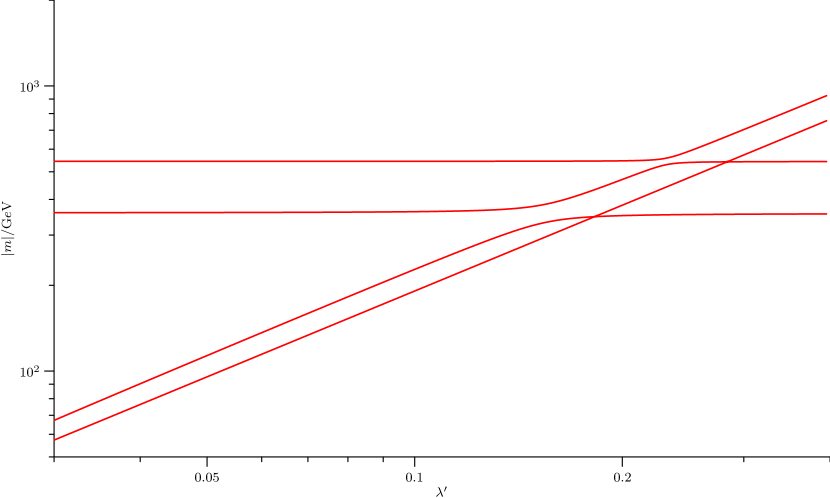
Figure 5.3 shows how the spectrum of chargino masses varies with $\lambda^{\prime}$. Although the plot is for $\tan(\beta)=1.5$, as one can see from (5.47) the inert sector of the chargino mass matrix has no dependence on $\tan(\beta)$, with the mass terms just being proportional to the SM-singlet VEV. The almost constant masses are those mass eigenvalues coming mostly from the USSM sector — the third generation charged Higgsino and the wino. The charginos coming mostly from the inert sector vary with $\lambda^{\prime}$ as expected and drop below the LEP lower limit around 100 GeV [93] at some value of $\lambda^{\prime}$, depending on the value of $s$. The effect of the $\epsilon=0.1$ mixing between generations can be seen in the splitting between the two inert sector charginos. Where lines cross in figure 5.3 the chargino masses are of opposite sign. When chargino mass lines of the same sign approach each other, they veer away from each other at the would-be crossing point due to interference.

Figure 5.4: Inert neutralino masses (magnitude only) against $\lambda^{\prime}$ with $f=1$, $\epsilon=0.1$, $\tan(\beta)=1.5$, $s=3000$ GeV, and $\mathds{Z}^{H}_{2}$-breaking $\lambda_{ijk}$ couplings set to 0.01.

Figure 5.4 shows how the spectrum of neutralino masses varies with $\lambda^{\prime}$. The inert neutralino spectrum is dependent on $\tan(\beta)$, but each of the qualitative features can be understood. We see the two light neutralino states that become heavier as $\lambda^{\prime}$ decreases from unity until the approximation $\lambda^{\prime}s\gg fv$ breaks down. At this point $fv\sin(\beta)$ begins to dominate and the LSP mass decreases with decreasing $\lambda^{\prime}$ as the dominance of $fv\sin(\beta)$ becomes greater. In this low $\lambda^{\prime}$ region the LSP is no longer mostly inert singlino, but is mostly inert up-type Higgsino. The six almost unvarying neutralino masses are those mostly from the USSM sector, which is not mixing very much with the inert sector. We have already seen that the inert sector chargino masses continue to be set by $\lambda^{\prime}$ as we go down into the low $\lambda^{\prime}$ region, resulting in light charginos in this region. By contrast, the four heavier inert sector neutralinos begin to be governed by the $fv$ terms rather than the $\lambda^{\prime}s$ terms in the low $\lambda^{\prime}$ region and therefore approach a constant value in this region.

As in the case of the charginos, the effect of the $\epsilon=0.1$ mixing can be seen in the splitting between the two light neutralinos and the four heavier inert neutralinos which are both split by this mixing and further split by the light neutralino mass as predicted in the previous section.

Figure 5.5: The component structure of the LSP in terms of the inert interaction states against $\lambda^{\prime}$ with $f=1$, $\epsilon=0.1$, $\tan(\beta)=1.5$, $s=3000$ GeV, and $\mathds{Z}^{H}_{2}$-breaking $\lambda_{ijk}$ couplings set to 0.01.

Figure 5.5 shows how the composition of the LSP in terms of the inert interaction states varies with $\lambda^{\prime}$. The behaviour in the $\lambda^{\prime}s\gg fv$ limit is as predicted in (5.64). We also see how the dominant component of the LSP changes from inert singlino to inert up-type Higgsino in the low $\lambda^{\prime}$ region.

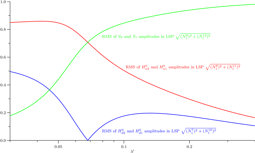
5.4.3 The dark matter relic density

Figure 5.6: Contour plot of the LSP mass and relic density $\Omega_{{\chi}}h^{2}$ regions in the $(\lambda^{\prime},\tan(\beta))$-plane with $s=3000$ GeV, $\epsilon=0.1$, and $f=1$. The red region is where the prediction for $\Omega_{{\chi}}h^{2}$ is consistent with the measured 1-sigma range of $\Omega_{\mathrm{DM}}h^{2}$. In the region to the right of the hatched line the LSP mass is less than half of the $Z$ boson mass.

Figure 5.7: Contour plot of the LSP mass and relic density $\Omega_{{\chi}}h^{2}$ regions in the $(\lambda^{\prime},f)$-plane with $s=3000$ GeV, $\epsilon=0.1$, and $\tan(\beta)=1.5$. The red region is where the prediction for $\Omega_{{\chi}}h^{2}$ is consistent with the measured 1-sigma range of $\Omega_{\mathrm{DM}}h^{2}$. In the region to the right of the hatched line the LSP mass is less than half of the $Z$ boson mass.

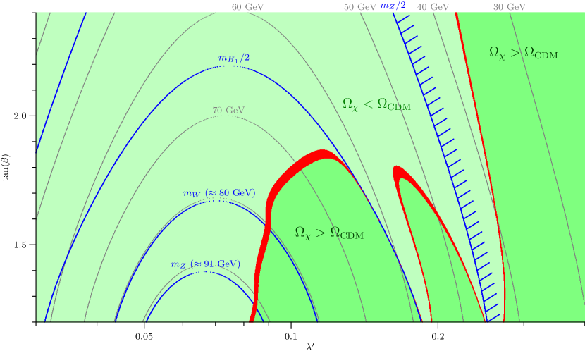
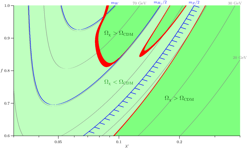
Using the parametrisation in (5.83) and (5.84) we use micrOMEGAs 2.2 to numerically compute the present day relic density. Figure 5.6 shows a contour plot of the LSP mass and predicted relic density $\Omega_{{\chi}}h^{2}$ regions in the $(\lambda^{\prime},\tan(\beta))$-plane, with $s=3000$ GeV, $\epsilon=0.1$, and $f=1$. We focus on small values of $\lambda^{\prime}<0.4$ since for large $\lambda^{\prime}$ the LSP is a very light, predominantly inert singlino state which does not annihilate very efficiently through any channel, leading to a too high relic density $\Omega_{{\chi}}h^{2}>\Omega_{\mathrm{DM}}h^{2}$. (Such regions are shaded dark green.) As $\lambda^{\prime}$ is decreased below 0.3 the LSP mass increases and approaches about half of the $Z$ boson mass and there is a region where the prediction for $\Omega_{{\chi}}h^{2}$ is consistent with the measured 1-sigma range of $\Omega_{\mathrm{DM}}h^{2}$. (Such regions are shaded red.) When the LSP mass is around 40 GeV it contains enough inert doublet Higgsino such that s-channel annihilation via the $Z$ boson becomes strong enough to account for the observed relic density. As the LSP mass is increased further from 40 GeV and approaches 45 GeV, the annihilations before freeze-out become on resonance for annihilation with a $Z$ boson in the s-channel and the predicted relic density becomes lower than that observed. (Such regions are shaded light green.)

In the regions where the LSP mass is less than half of the $Z$ boson mass the LSP will contribute to the effective number of neutrinos as inferred from the invisible $Z$ boson width at LEP defined in (1.23). The same couplings that lead to a successful relic density, via annihilations through an s-channel $Z$ boson, also mean that there may be a significant contribution to the invisible $Z$ boson width. For the present discussion it is assumed that such points, with an LSP mass lower that half of the $Z$ mass, are unsafe from an experimental point of view. A detailed discussion of the validity of such points is postponed until chapter 6. Note that in the MSSM this issue does not arise since either the LSP is bino-like, and so does not couple to the $Z$, or is Higgsino- or Wino-like in which case it would have accompanying almost degenerate charginos and therefore must have a mass greater than about 100 GeV in any case. Here we can have an inert Higgsino/singlino LSP with a mass lower than half of the $Z$ boson mass while still having experimentally consistent inert-doublet-Higgsino-like charginos.

We note at this point that the requirement that the LSP mass exceeds 45 GeV implies low $\tan(\beta)$ and this is the reason for the restricted range of $\tan(\beta)$ in figure 5.6. This can be seen from (5.54) where we found that the LSP mass should be approximately proportional to $\sin(2\beta)$, i.e. to the product of the two doublet Higgs VEVs, which is maximized at $\sin(2\beta)=1$, corresponding to $\tan(\beta)=1$. In the $E_{6}$SSM an experimentally acceptable lightest Higgs mass can be achieved even with $\tan(\beta)$ as low as about 1.2 [55], so having low $\tan(\beta)$ is not a problem in such models.

Decreasing $\lambda^{\prime}$ further results in LSP masses above 45 GeV and to the left of the hatched line in figure 5.6 other successful relic density regions (shaded in red) appear. These regions are punctuated by the light Higgs resonance, leading to the interesting double loop shape of the successful red regions to the left of the hatched line in figure 5.6. In these regions the LSP can have a mass significantly larger than half of the $Z$ boson mass, moving far enough off the Higgs and $Z$ boson resonances that annihilation is weakened just enough to give the observed relic density.

However, another effect is observed as $\lambda^{\prime}$ decreases. The composition of the LSP changes from being singlino dominated to being Higgsino dominated. For low $\lambda^{\prime}$ the cross-section begins to increase with decreasing $\lambda^{\prime}$, even where this still corresponds to increasing LSP mass, leading to a lower relic density. This is because the inert doublet Higgsino components in the LSP rapidly grow, as can be seen in figure 5.5. At low $\lambda^{\prime}$, when the LSP is largely inert doublet Higgsino, annihilation is too strong, leading to the predicted relic density being lower than that observed (as indicated by the light green shading in figure 5.6). The effects of the t-channel $W$ and then $Z$ pair production channels can also be seen as they each become relevant.

Furthermore, for the entire successful region to the left of the hatched line in figure 5.6 the lightest chargino is heavy enough to be consistent with experiment, as can be seen on figure 5.3. This result will be recreated for all high enough values of $s$. For larger values of $s$ the successful regions and corresponding inert chargino masses are shifted down by the corresponding amount in $\lambda^{\prime}$.

When $\lambda^{\prime}s\gg fv$ lowering $f$ results in a lower LSP mass, as in (5.54). It also extends the range of $\lambda^{\prime}$ in which this approximation is valid, i.e. it moves the boundary of the previously discussed low $\lambda^{\prime}$ region to be further down in $\lambda^{\prime}$. Figure 5.7 shows the LSP mass and predicted present day relic density for different values of $\lambda^{\prime}$ and $f$ with $\epsilon=0.1$ and $\tan(\beta)=1.5$. The shifting of the successful region, where the LSP mass is above $m_{Z}/2$, down in $\lambda^{\prime}$ at lower values of $f$ is apparent. At lower values of $\tan(\beta)$ this successful region extends further down in $f$. It should be noted that in order to predict the correct dark matter relic density, $\lambda^{\prime}$ should be much smaller than $f$ and that this disparity becomes greater if $s$ is increased. Increasing $s$ effectively just shifts all of the features on figures 5.6 and 5.7 to the left.

5.4.4 Deviations from the considered parametrisation

Breaking the relation $f_{u(22,11)}=f_{d(22,11)}$ can have similar effects to those of changing $\tan(\beta)$. However, because these parameters cannot be too high (in order for the theory to be perturbative up to the GUT scale) and because lowering them to much less than unity makes the LSP too light, $\tan(\beta)$ can be varied much more freely than the $f_{u}/f_{d}$ ratio.

The effect of increasing the inert generation mixing parameter $\epsilon$ is to increase the various mass splittings between similar inert mass eigenstates. Increasing the mixing between the first and second generations thus results in a lighter LSP, shrinking the successful region, and a lighter lightest chargino, potentially inconsistent with current chargino non-observation.

The physics of the inert sector when deviating from the currently considered parametrisation is studied much more carefully in chapter 6.

As long as the LSP is still mostly from the inert sector, as considered here, other parameters do not greatly affect the dark matter physics and are effectively free. Squark and slepton parameters do not affect the dark matter physics of the considered model. Top and stop loops can have a significant effect on the lightest Higgs mass, but as long as this mass is experimentally allowed then these parameters are also not constrained by the requirement that the model produce successful dark matter.

5.5 Summary and Conclusions

In this work we studied inert neutralino dark matter arising in supersymmetric models with extra inert Higgsinos and singlinos. As an example we considered the extended neutralino sector of the $E_{6}$SSM. This work represents a first study of the inert neutralino sector of the $E_{6}$SSM and it is found that in this model the LSP does typically arise from this sector. We studied this novel dark matter scenario both analytically and numerically, using micrOMEGAs.

The dark matter scenario differs greatly from those of the MSSM and USSM since the two inert neutralino generations provide an almost decoupled neutralino sector with a naturally light LSP that can account for the CDM relic abundance somewhat independently of the rest of the model. Although the $E_{6}$SSM has two inert generations, the presence of the second inert generation is not crucial to the dark matter scenario.

In the successful regions where the observed dark matter relic density is reproduced the neutralino mass spectrum is well described by the analytical results of section 5.3. In this region the LSP is mostly inert singlino and has a mass approximately proportional to $v^{2}/s$, as in (5.54), and as $\lambda^{\prime}s$ is decreased the LSP becomes heavier and also less inert singlino dominated, picking up significant inert doublet Higgsino contributions.

To avoid potential conflict with high precision LEP data we considered the case where the LSP mass is above half of the $Z$ boson mass. Since the LSP mass in (5.54) is proportional to $f_{d}f_{u}\sin(2\beta)$, we found that such regions of parameter space in which the dark matter relic density prediction is consistent with observation require low values of $\tan(\beta)$ — less than about 2. Depending on the value of the singlet VEV $s$, the $f_{(u,d)\alpha\beta}$ trilinear Higgs coupling parameters should also be reasonably large compared to the $\lambda_{\alpha\beta}$ ones.

One of the main messages arising from this work is that neutralino dark matter could arise from an almost decoupled sector of inert Higgsinos and singlinos and that if it does then the parameter space of the rest of the model is completely opened up. For example, if such a model is regarded as an extension of the MSSM then the lightest MSSM-like supersymmetric particle is not even required to be a neutralino and could even be a sfermion. In the $E_{6}$SSM the lightest MSSM-like supersymmetric particle can decay into the inert LSP via $\mathds{Z}^{H}_{2}$-breaking $\lambda_{ijk}$ couplings that need not be extremely small.

Similar results should apply to any singlet extended SSM with one or more extra, inert generations of Higgsinos and singlinos with a trilinear Higgs coupling tensor equivalent to that in (5.1).

Chapter 6 Novel Higgs Decays in the $E_{6}$SSM

The discovery of the Higgs boson, the last remaining undiscovered particle of the SM, is one of the main goals of the LHC. The strategy for Higgs searches depends on the decay branching fractions of the Higgs boson into different channels. Physics beyond the SM may affect the Higgs decay rates to SM particles and give rise to new Higgs decay channels necessitating a drastic change in the strategy for Higgs boson searches. (For recent reviews of non-standard Higgs boson decays see refs. [94, 95, 96].) In particular there exist several extensions to the SM in which the Higgs boson can decay with a substantial branching fraction into particles that cannot be directly detected.

These invisible Higgs boson decays can occur in supersymetry, with the lighest Higgs boson decaying into neutralino LSPs. In some regions of MSSM parameter space the lightest Higgs boson decays into the lightest neutralino with a relatively large branching ratio, giving rise to invisible final states if $R$-parity is conserved [97]. LEP and Tevatron data allow the neutralino LSP to be sufficiently light such that the decays of the lightest Higgs boson into these neutralinos is kinematically allowed and such light neutralinos can annihilate efficiently through a $Z$ boson pole resulting in a reasonable density of dark matter.

The presence of invisible decays considerably modifies Higgs boson searches and makes discovery much more difficult. If the Higgs boson is mainly invisible then the usual visible branching ratios will be dramatically reduced, preventing detection in the much studied channels at the LHC and Tevatron. In the case where invisible Higgs boson decays dominate it is impossible to fully reconstruct a resonance and it is very challenging to identify the Higgs boson at collider experiments, i.e. the quantum numbers remain unknown. At $e^{+}e^{-}$ colliders, the problems relating to the observation of an invisible Higgs boson are less severe [98, 99, 100] since it can be tagged through the recoiling $Z$. The LEP exclusion of Higgs boson masses up to 114.4 GeV applies even in the case of invisibly decaying Higgs bosons [101] and similar limits could apply to Higgs bosons decaying into soft lepton pairs some fraction of the time, as happens for some of the novel Higgs decay scenarios discussed in this chapter.

Higgs boson searches at hadron colliders, however, are more difficult in the presence of such invisible decays. Previous studies have analysed $Zh$ and $Wh$ associated production [102, 103, 104] as well as $t\bar{t}h$ production [105, 106] and $t\bar{t}VV$ and $b\bar{b}VV$ production [107] as promising channels, where $h$ is the Higgs boson and the $V$s stand for vector bosons. The possibility of observing an invisible Higgs boson in central exclusive diffractive production at the LHC was studied in [108]. Another proposal is to observe such an invisible Higgs in inelastic events with large missing transverse energy and two high $E_{T}$ jets. In this case the Higgs boson is produced by $VV$ fusion and has a large transverse momentum resulting in a signal with two quark jets with distinctive kinematic distributions compared to $Zjj$ and $Wjj$ backgrounds [109, 104, 110].

In this chapter, which contains work that was first published in paper II, we consider novel decays of the lightest Higgs boson and associated collider signatures within the $E_{6}$SSM. If the Yukawa couplings of the inert neutralino sector are required to be small enough such that perturbation theory remains valid up to the GUT scale then the masses of the two lightest inert neutralino states are expected to be smaller than about 60–65 GeV. As a result the lightest inert neutralino tends to be the LSP. As noted in the previous chapter such an inert neutralino can give an appropriate contribution to the dark matter density, consistent with recent observations, if it has a mass around 35–50 GeV. In this case the lightest Higgs boson decays predominantly into inert neutralino states and the usual Higgs boson branching ratios to SM particles are less than a few percent.

In section 6.1 we look in more detail at the inert sector of the model and the couplings of the inert neutralinos, inert charginos, and active Higgs bosons are specified. Novel decays of the lightest $CP$-even Higgs state and dark matter constraints are discussed in section 6.2. In section 6.3 we specify some benchmark points and discuss the experimental constraints and predictions. The conclusions are summarised in section 6.4.

6.1 Inert Charginos and Neutralinos

In our analysis we will assume that $\mathds{Z}^{H}_{2}$-violating couplings are small and can be neglected. This assumption can be justified if one takes into account that the $\mathds{Z}^{H}_{2}$-violating operators can give an appreciable contribution to the amplitude of $K^{0}$-$\bar{K}^{0}$ oscillations and give rise to new muon decay channels such as $\mu\rightarrow e^{-}e^{+}e^{-}$. In order to suppress processes with non-diagonal flavour transitions the Yukawa couplings of the exotic particles to the quarks and leptons of the first two generations should be smaller than $10^{-3}$–$10^{-4}$. Such small $\mathds{Z}^{H}_{2}$-violating couplings can be neglected in the first approximation.

In this approximation, and given the assumption that only $H_{u}$, $H_{d}$, and $S$ acquire non-zero VEVs, the charged components of the inert Higgsinos do not mix with the MSSM-like chargino states. The neutral components of the inert Higgsinos and inert singlinos also do not mix with the USSM-like neutralino states. If $\mathds{Z}^{H}_{2}$ symmetry was exact then both the lightest state in the ordinary neutralino sector and the lightest inert neutralino would be absolutely stable. Therefore although $\mathds{Z}^{H}_{2}$-violating couplings are expected to be rather small we shall assume that they are large enough to allow either the lightest USSM-like neutralino state or the lightest inert neutralino state to decay within a reasonable time — the lighter of the two being the stable LSP and the dark matter candidate.

In the basis

$$\tilde{N}^{\mathrm{int}}_{\mathrm{inert}} = \left(\begin{array}[]{cccccc}\tilde{H}^{0}_{d2}&\tilde{H}^{0}_{u2}&\tilde{S}^{\vphantom{0}}_{2}&\tilde{H}^{0}_{d1}&\tilde{H}^{0}_{u1}&\tilde{S}^{\vphantom{0}}_{1}\end{array}\right)^{\mathrm{T}}$$ (6.2)

the inert part of the neutralino mass matrix is given by

$$M^{N}_{\mathrm{inert}} = \left(\begin{array}[]{cc}A^{\vphantom{\mathrm{T}}}_{22}&A^{\vphantom{\mathrm{T}}}_{21}\\ A^{\mathrm{T}}_{21}&A^{\vphantom{\mathrm{T}}}_{11}\end{array}\right),$$ (6.5)

with the submatrices given in (5.20). The inert part of the chargino mass matrix $P$, given in (5.47), may be written

$$P^{\mathrm{inert}}_{\alpha\beta} = \dfrac{1}{\sqrt{2}}\lambda^{\vphantom{\mathrm{inert}}}_{\alpha\beta}.$$ (6.6)

From (6.5) and (6.6) one can see that in the exact $\mathds{Z}^{H}_{2}$ symmetry limit the spectrum of the inert neutralinos and charginos in the $E_{6}$SSM can be parametrised in terms of $\lambda_{\alpha\beta}$, $f_{d\alpha\beta}$, $f_{u\alpha\beta}$, $\tan(\beta)$, and $s$. In other words the masses and couplings of the inert neutralinos are determined by 12 Yukawa couplings, which can in principle be complex, $\tan(\beta)$, and $s$. Four of the Yukawa couplings mentioned above — $\lambda_{\alpha\beta}$ — as well as the VEV of the SM singlet field $s$ set the masses and couplings of the inert chargino states. Six off-diagonal Yukawa couplings define the mixing between the two generations of inert Higgsinos and singlinos.

In the following analysis the VEV of the active SM-singlet field is chosen to be large enough ($s\gtrsim 2400$ GeV) so that experimental constraints from ref. [67] on the $Z_{2}$ boson mass ($m_{{}_{Z_{2}}}>892$ GeV) and $Z$-$Z^{\prime}$ mixing are satisfied. Since the publication of paper II the limit on the $Z_{2}$ mass in the $E_{6}$SSM has increased as discussed in subsection 3.2.2. In order to avoid the LEP lower limit on the masses of inert charginos [93] the Yukawa couplings $\lambda_{\alpha\beta}$ are chosen such that all inert chargino states are heavier than $100$ GeV. In addition, we also require the validity of perturbation theory up to the GUT scale and this constrains the allowed range of all Yukawa couplings.

The theoretical and experimental restrictions specified above set very strong limits on the masses and couplings of the lightest inert neutralinos. In particular, our numerical analysis indicates that the lightest and second lightest inert neutralinos are always light. They typically have masses below 60–65 GeV. These neutralinos are predominantly inert singlino in nature. From our numerical analysis it follows that the lightest and second lightest inert neutralinos might have rather small couplings to the $Z$ boson so that any possible signal that these neutralinos could give rise to at LEP would be extremely suppressed. As a consequence such inert neutralinos would remain undetected. At the same time four other inert neutralinos, which are approximately linear superpositions of neutral components of inert doublet Higgsinos, are normally heavier than 100 GeV.

6.1.1 The diagonal inert Yukawa coupling approximation

In order to clarify the results of our numerical analysis it is useful to consider a few simple cases that give some analytical understanding of our calculations. The simplest case is when all of the Yukawa coupling from the off-diagonal blocks of (6.5) are zero such that

$$\lambda_{\alpha\beta} = \lambda_{\alpha}\delta_{\alpha\beta},$$

$$f_{d\alpha\beta} = f_{d\alpha}\delta_{\alpha\beta},\quad\mbox{and}$$

$$f_{u\alpha\beta} = f_{\alpha}\delta_{\alpha\beta}\quad\mbox{(no sum on $\alpha$)}.$$ (6.7)

This leads to two decoupled generations with the properties studied in section 5.3. The mass matrix of inert neutralinos (6.5) reduces to block diagonal form while the masses of the inert charginos are given by

$$m_{\tilde{C}_{\alpha}} = \dfrac{\lambda_{\alpha}}{\sqrt{2}}s.$$ (6.8)

When $f_{\alpha}=f_{d\alpha}=f_{u\alpha}$ one can prove using the method proposed in ref. [111] that there are theoretical upper bounds on the masses of the lightest and second lightest inert neutralino states. The theoretical restrictions are $|m_{\tilde{N}_{\alpha}}|^{2}\lesssim\mu_{\alpha}^{2}$, where

$$\mu_{\alpha}^{2} = \dfrac{1}{2}\left[|m_{\tilde{C}_{\alpha}}|^{2}+\dfrac{f_{\alpha}^{2}v^{2}}{2}\Big{(}1+\sin^{2}(2\beta)\Big{)}\vphantom{\sqrt{\left(|m_{\tilde{C}_{\alpha}}|^{2}+\dfrac{f_{\alpha}^{2}v^{2}}{2}(1+\sin^{2}(2\beta))\right)^{2}-f_{\alpha}^{4}v^{4}\sin^{2}(2\beta)}}\right.$$ (6.9)

$$\quad\vphantom{A}-\left.\sqrt{\left(|m_{\tilde{C}_{\alpha}}|^{2}+\dfrac{f_{\alpha}^{2}v^{2}}{2}\Big{(}1+\sin^{2}(2\beta)\Big{)}\right)^{2}-f_{\alpha}^{4}v^{4}\sin^{2}(2\beta)}\right].$$

The value of $\mu_{\alpha}$ decreases with increasing $|m_{\tilde{C}_{\alpha}}|$ and $\tan(\beta)$, approaching its maximum value

$$\mu_{\alpha} \rightarrow \dfrac{f_{\alpha}}{\sqrt{2}}v$$ (6.10)

as $m_{\tilde{C}_{\alpha}}\rightarrow 0$ and $\tan(\beta)\rightarrow 1$.

The upper bound on the mass of the lightest inert neutralino also depends on the values of the Yukawa couplings $f_{d\alpha}$ and $f_{u\alpha}$. The theoretical restrictions on these couplings due to the requirement that the theory should remain perturbative up to the GUT scale become weaker with increasing $\tan(\beta)$. At large values of $\tan(\beta)$ the upper bounds on $|m_{\tilde{C}_{\alpha}}|$ from (6.9) becomes rather small and as $\tan(\beta)$ tends to unity the upper bounds on $|m_{\tilde{C}_{\alpha}}|$ again become rasther small, because theoretical constraints on $f_{d\alpha}$ and $f_{u\alpha}$ become rather stringent. Taking both of these effects in account the upper bounds on $|m_{\tilde{C}_{\alpha}}|$ achieve their maximum values around $\tan(\beta)\approx 1.5$. For this value of $\tan(\beta)$ the requirement of the validity of perturbation theory up to the GUT scale implies that for $f=f_{d1}=f_{u1}=f_{d2}=f_{u2}$ $f$ must be less than about $0.6$. As a consequence the lightest inert neutralinos are lighter than around $60$–$65$ GeV for $|m_{\tilde{C}_{\alpha}}|>100$ GeV.

Using the results from section 5.3 for the compositions of the light neutralinos from each inert generation one can derive the couplings of these states to the $Z$ boson. We define $R_{Z\alpha\beta}$ couplings such that the $Z$-$\tilde{N}_{\alpha}$-$\tilde{N}_{\beta}$ coupling is equal to $R_{Z\alpha\beta}$ times the $Z$-$\nu$-$\nu$ coupling

$$R_{Z\alpha\beta} = N_{\alpha}^{1}N_{\beta}^{1}-N_{\alpha}^{2}N_{\beta}^{2}+N_{\alpha}^{4}N_{\beta}^{4}-N_{\alpha}^{5}N_{\beta}^{5},$$ (6.11)

where $N_{i}^{a}$ is the neutralino mixing matrix element corresponding to mass eigenstate $i$ and inert interaction state $a$ in the basis (6.2).

In the case where the off-diagonal inert Yukawa coupling blocks vanish while $\lambda_{\alpha}s\gg f_{(u,d)\alpha}v$ the relative couplings of the lightest and second lightest inert neutralino states to the $Z$ boson are given by

$$R_{Z\alpha\beta} = R_{Z\alpha\alpha}\delta_{\alpha\beta}\quad\mbox{(no sum on $\alpha$)},$$ (6.12)

where

$$R_{Z\alpha\alpha} = \dfrac{v^{2}}{2m_{\tilde{C}_{\alpha}}^{2}}\biggl{(}f_{d\alpha}^{2}\cos^{2}(\beta)-f_{u\alpha}^{2}\sin^{2}(\beta)\biggr{)}.$$ (6.13)

This demonstrates that the couplings of $\tilde{N}_{1}$ and $\tilde{N}_{2}$ to the $Z$ boson can be very strongly suppressed. It becomes zero when $|f_{d\alpha}|\cos(\beta)=|f_{u\alpha}|\sin(\beta)$, which is when $\tilde{N}_{\alpha}$ contains a completely symmetric combination of $\tilde{H}^{0}_{d\alpha}$ and $\tilde{H}^{0}_{u\alpha}$. (6.13) also indicates that the couplings of $\tilde{N}_{1}$ and $\tilde{N}_{2}$ to the $Z$ boson are always small if the inert charginos are rather heavy or if $f_{d\alpha}$ and $f_{u\alpha}$ are small, i.e. the masses of $\tilde{N}_{1}$ and $\tilde{N}_{2}$ are small.

6.1.2 $\Delta_{27}$ and pseudo-Dirac lightest inert neutralino states

In order to provide an explanation for the origin of the approximate $\mathds{Z}^{H}_{2}$ symmetry that singles out the third generation of Higgs doublets and SM-singlets, and to account for tribimaximal mixing and other features of the quark and lepton spectra, a $\Delta_{27}$ flavour symmetry may be applied to the $E_{6}$SSM [59]. The addition of the $\Delta_{27}$ flavour symmetry implies an inert neutralino mass matrix with $A_{11}\approx A_{22}\approx 0$, leading to approximately degenerate lightest neutralino states with a pseudo-Dirac (see appendix A) structure.

When all flavour diagonal Yukawa couplings $\lambda_{\alpha\alpha}$, $f_{d\alpha\alpha}$, and $f_{u\alpha\alpha}$ exactly vanish, i.e. $A_{11}=A_{22}=0$, the inert neutralinos form Dirac states. In this limit the Lagrangian of the $E_{6}$SSM is invariant under an extra $U(1)$ global symmetry. Under this symmetry the fermionic components of the inert supermultiplets transform

$$\tilde{S}_{2} \rightarrow e^{i\alpha}\tilde{S}_{2},$$

$$\tilde{H}_{d2} \rightarrow e^{i\alpha}\tilde{H}_{d2},$$

$$\tilde{H}_{u2} \rightarrow e^{i\alpha}\tilde{H}_{u2},$$

$$\tilde{S}_{1} \rightarrow e^{-i\alpha}\tilde{S}_{1},$$

$$\tilde{H}_{d1} \rightarrow e^{-i\alpha}\tilde{H}_{d1},$$

$$\tilde{H}_{u1} \rightarrow e^{-i\alpha}\tilde{H}_{u1}.$$ (6.14)

In the above limiting case the lightest inert neutralino is a Dirac state formed predominantly from $\tilde{S}_{1}$ and $\tilde{S}_{2}$. In this case the LSP and its antiparticle have opposite charges with respect to the extra global $U(1)$ and this could lead to the scenario known as asymmetric dark matter [112, 113, 114, 115]. The ADM scenario supposes that there could be an asymmetry between the density of dark matter particles and their antiparticles in the early universe similar to that for baryons. This could have a considerable effect on the relic density calculations. In particular, if an asymmetry exists between the number densities of dark matter particles and their antiparticles in the early universe then one can get an appreciable dark matter density even if the dark matter particle-antiparticle annihilation cross section is very large, like in the case of baryons. Furthermore, if most of the dark matter antiparticles are eliminated by annihilation with their particles then such an ADM scenario does not have the usual indirect signatures associated with the presence of dark matter. For example, there would be no high energy neutrino signal from annihilations in the Sun. At the same time, a relatively high concentration of dark matter particles can build up in the Sun, altering heat transport in the solar interior and affecting low energy neutrino fluxes [115].

In practice the $\Delta_{27}$ scenario tells us that we are somewhat away from the above limiting case, with a broken global $U(1)$ symmetry leading to almost degenerate pseudo-Dirac lightest neutralinos, where the relic density of the LSP can be calculated by standard methods. It will turn out that the LSP cannot be too light (must be of order $m_{Z}/2$) in order not to have a too high cosmological relic density. At the same time we will see that the two lightest neutralinos cannot be too heavy in order for perturbation theory to be valid up to the GUT scale. In practice this means that in realistic scenarios the two lightest inert neutralino states are rather close in mass. The $\Delta_{27}$ scenario provides an explanation for this feature of the successful neutralino mass pattern.

It is worth noting that the results from the previous section can be reinterpreted in terms of this scenario. Specifically in the case where $A_{11}=A_{22}=0$ and $A_{21}=A_{12}$ a block diagonalisation of the inert neutralino mass matrix (6.5) results in

$$\begin{array}[]{c}A_{22}\rightarrow A_{22}^{\prime}=-A_{21},\qquad\mbox{and}\qquad A_{11}\rightarrow A_{11}^{\prime}=A_{21},\end{array}$$ (6.15)

with $A_{21}=A_{12}\rightarrow A_{21}^{\prime}=A_{12}^{\prime}=0$. This only corresponds to a redefinition of the generations 1 and 2 and does not mix fields of different hypercharge. This provides a dictionary between these two scenarios

$$-\lambda_{22}^{\prime}=\lambda_{11}^{\prime} = \lambda_{21},$$

$$-f_{d22}^{\prime}=f_{d11}^{\prime} = f_{d21},$$ (6.16)

$$-f_{u22}^{\prime}=f_{u11}^{\prime} = f_{u21}.$$ (6.17)

Rewriting the inert neutralino mass matrix in this block diagonal form also makes it clear that the $R_{Z12}$ coupling vanishes in this limit in the same way that it did for the diagonal case in subsection 6.1.1.

6.1.3 The couplings of Higgs bosons to inert neutralinos

The presence of light inert neutralinos in the particle spectrum of the $E_{6}$SSM makes possible the decays of the Higgs bosons into these final states. Now and in the next section we argue that such decays may result in the modification of the SM-like Higgs signal at current and future colliders. Since our main concern in this work is the decays of the SM-like lightest Higgs boson, we shall ignore the effects of the inert Higgs scalars and pseudoscalars which do not mix appreciably with the active scalar sector responsible for EWSB. We also assume that all of the inert bosons are heavier than the lightest $CP$-even Higgs boson.

If all other Higgs boson states are much heavier than the lightest $CP$-even Higgs boson then the lightest Higgs state, approximately given by $h$, as defined in (3.30), manifests itself in interactions with SM gauge bosons and fermions as a SM-like Higgs boson. Since within the $E_{6}$SSM the mass of this state is predicted to be relatively low, its production cross section at the LHC should be large enough so that it can be observed in the near future. In this context it is particularly interesting and important to analyse the decay modes of the lightest $CP$-even Higgs state. Furthermore, we concentrate on the decays of the SM-like Higgs boson into the lightest and second lightest inert neutralinos.

The couplings of the Higgs states to the inert neutralinos originate from the interactions of $H_{u}$, $H_{d}$, and $S$ with the inert Higgs fields in the superpotential. Using (3.30) one can express $\mathfrak{Re}\,H_{d}^{0}$, $\mathfrak{Re}\,H_{u}^{0}$, and $\mathfrak{Re}\,S$ in terms of the field-space basis states $h$, $H$, and $N$. The components of the field-space basis are related to the physical $CP$-even mass eigenstates by a unitary transformation

$$\left(\begin{array}[]{c}h_{1}\\ h_{2}\\ h_{3}\end{array}\right) = U\left(\begin{array}[]{c}h\\ H\\ N\end{array}\right).$$ (6.24)

Combining all these expressions together one obtains an effective Lagrangian term that describes the interactions of the inert neutralinos with the $CP$-even Higgs mass eigenstates

$$\begin{array}[]{c}X^{h_{m}}_{ij}h_{m}\tilde{N}^{c\dagger}_{i}\tilde{N}^{\vphantom{\dagger}}_{j}+\mbox{c.c.},\end{array}$$ (6.25)

where

$$X^{h_{m}}_{ij} = -\dfrac{1}{\sqrt{2}}U^{N}_{h_{m}}\Lambda^{\vphantom{N}}_{ij}-\dfrac{1}{\sqrt{2}}\left(U^{h}_{h_{m}}\cos(\beta)-U^{H}_{h_{m}}\sin(\beta)\right)F^{\vphantom{N}}_{dij}$$ (6.26)

$$\qquad\vphantom{A}-\dfrac{1}{\sqrt{2}}\left(U^{h}_{h_{m}}\sin(\beta)+U^{H}_{h_{m}}\cos(\beta)\right)F^{\vphantom{N}}_{uij},$$

with

$$\Lambda^{\vphantom{N}}_{ij} = \lambda^{\vphantom{1}}_{11}N^{4}_{i}N^{5}_{j}+\lambda^{\vphantom{1}}_{12}N^{4}_{i}N^{2}_{j}+\lambda^{\vphantom{1}}_{21}N^{1}_{i}N^{5}_{j}+\lambda^{\vphantom{1}}_{22}N^{1}_{i}N^{2}_{j},$$ (6.27)

$$F^{\vphantom{N}}_{dij} = f^{\vphantom{1}}_{d11}N^{6}_{i}N^{5}_{j}+f^{\vphantom{1}}_{d12}N^{6}_{i}N^{2}_{j}+f^{\vphantom{1}}_{d21}N^{3}_{i}N^{5}_{j}+f^{\vphantom{1}}_{d22}N^{3}_{i}N^{2}_{j},\quad\mbox{and}$$ (6.28)

$$F^{\vphantom{N}}_{uij} = f^{\vphantom{1}}_{u11}N^{6}_{i}N^{5}_{j}+f^{\vphantom{1}}_{u12}N^{6}_{i}N^{2}_{j}+f^{\vphantom{1}}_{u21}N^{3}_{i}N^{5}_{j}+f^{\vphantom{1}}_{u22}N^{3}_{i}N^{2}_{j}.$$ (6.29)

The expressions for the couplings of the active $CP$-even Higgs scalars to the inert neutralinos become much simpler in the case where the Higgs spectrum has the usual hierarchical structure. In this case $U$ is almost the identity. As a consequence the couplings of the SM-like Higgs boson to the lightest and second lightest inert neutralino states are approximately given by

$$X^{h_{1}}_{\alpha\beta} = -\dfrac{1}{\sqrt{2}}\Big{(}F_{d\alpha\beta}\cos(\beta)+F_{u\alpha\beta}\sin(\beta)\Big{)}.$$ (6.30)

In the case of the diagonal inert Yukawa coupling limit defined in subsection 6.1.1 and if $\lambda_{\alpha}s\gg f_{(d,u)\alpha}v$ one can use the expression (5.64) to find values for $N^{a}_{1}$ and $N^{a}_{2}$ and derive approximate formulae for $X^{h_{1}}_{\alpha\beta}$. Substituting into (6.30) one obtains

$$X^{h_{1}}_{\alpha\beta} = \dfrac{m_{\tilde{N}_{\alpha}}}{v}\delta_{\alpha\beta}+\cdots\quad\mbox{(no sum on $\alpha$)}.$$ (6.31)

This simple analytical expression for the couplings of the SM-like Higgs boson to the lightest and second lightest inert neutralinos is not as surprising as it may first appear. When the Higgs spectrum is hierarchical, with $s\gg v$, the VEV of the lightest $CP$-even state $v$ is responsible for all light fermion masses in the $E_{6}$SSM. As a result we expect that their couplings to the SM-like Higgs can be written as usual as being proportional to the mass divided by the VEV. We see that this is exactly what is found in the limit of $m_{\tilde{N}_{\alpha}}$ being small.

6.2 Novel Higgs Decays and Dark Matter

The interaction Lagrangian (6.25) gives rise to decays of the lightest Higgs boson into inert neutralino pairs with partial widths given by

$$\Gamma(h_{1}\rightarrow\tilde{N}_{\alpha}\tilde{N}_{\beta}) = \dfrac{\Delta_{\alpha\beta}}{16\pi m_{h_{1}}}\biggl{(}X^{h_{1}}_{\alpha\beta}+X^{h_{1}}_{\beta\alpha}\biggr{)}^{2}\biggl{[}m_{h_{1}}^{2}-(m_{\tilde{N}_{\alpha}}-m_{\tilde{N}_{\beta}})^{2}\biggr{]}$$ (6.32)

$$\quad\sqrt{\left(1-\dfrac{m_{\tilde{N}_{\alpha}}^{2}}{m_{h_{1}}^{2}}-\dfrac{m_{\tilde{N}_{\beta}}^{2}}{m_{h_{1}}^{2}}\right)^{2}-4\dfrac{m_{\tilde{N}_{\alpha}}^{2}m_{\tilde{N}_{\beta}}^{2}}{m_{h_{1}}^{4}}},$$

where $\Delta_{\alpha\beta}=\{1,2\}$ for {$\alpha=\beta$, $\alpha\neq\beta$}.

The partial widths associated with these inert decays of the SM-like Higgs boson (6.32) have to be compared to decay rates into SM particles. When the SM Higgs boson is relatively light (less than about 140 GeV) it decays predominantly into $b$ quark and $\tau$ lepton pairs. The partial decay width of the lightest $CP$-even Higgs boson into Dirac fermion pairs is given by [116]

$$\Gamma(h_{1}\rightarrow f\bar{f}) = N_{c}\dfrac{\vphantom{m^{2}_{f}}g_{2}^{2}}{32\pi}\dfrac{m^{2}_{f}}{m^{2}_{W}}g^{2}_{h_{1}ff}m^{\vphantom{2}}_{h_{1}}\biggl{(}1-4\dfrac{m_{f}^{2}}{m_{h_{1}}^{2}}\biggr{)}^{3/2}.$$ (6.33)

For the case of the decays into $\tau$ leptons the coupling of the lightest $CP$-even Higgs state to the $\tau$ lepton normalised to the corresponding SM coupling

$$g_{h_{1}\tau\tau} = \dfrac{1}{\cos(\beta)}\biggl{(}U^{h}_{h_{1}}\cos(\beta)-U^{H}_{h_{1}}\sin(\beta)\biggr{)}.$$ (6.34)

For a final state that involves $b$ quarks one has to include the QCD corrections. In particular, the fermion mass in (6.33) should be associated with the running $b$ quark mass $\bar{m}_{b}(\mu)$. The bulk of the QCD corrections are absorbed by using the running $b$ quark mass defined at the appropriate renormalisation scale — the scale of the lightest Higgs boson mass $\mu=m_{h_{1}}$ in the considered case. In addition to the corrections that are associated with the running $b$ quark mass there are other QCD corrections to the Higgs coupling to $b$ quarks that should be taken into account [117]. As a consequence, the partial decay width of the lightest $CP$-even Higgs boson into $b$ quark pairs can be calculated using (6.33) if one sets

$$N_{c} = 3,$$

$$m_{f} = \bar{m}_{b}(m_{h_{1}}),\quad\mbox{and}$$ (6.35)

$$g^{2}_{h_{1}ff} = \dfrac{1}{\cos^{2}(\beta)}\biggl{(}U^{h}_{h_{1}}\cos(\beta)-U^{H}_{h_{1}}\sin(\beta)\biggr{)}^{2}\biggl{[}1+\Delta_{bb}+\Delta_{H}\biggr{]},$$

where

$$\Delta_{bb} \approx 5.67\dfrac{\bar{\alpha}_{s}(m_{h_{1}})}{\pi}+(35.94-1.36N_{f})\dfrac{\bar{\alpha}^{2}_{s}(m_{h_{1}})}{\pi^{2}}\quad\mbox{and}$$

$$\Delta_{H} \approx \dfrac{\bar{\alpha}^{2}_{s}(m_{h_{1}})}{\pi^{2}}\left(1.57-\dfrac{2}{3}\ln\left(\dfrac{m_{h_{1}}^{2}}{m_{t}^{2}}\right)+\dfrac{1}{9}\ln^{2}\left(\dfrac{\bar{m}_{b}^{2}(m_{h_{1}})}{m_{h_{1}}^{2}}\right)\right).$$

Here we neglect radiative corrections that originate from loop diagrams that contain non-SM particles.

From (6.31) one can see that in the $E_{6}$SSM the branching ratios of the SM-like Higgs state into the lightest and second lightest inert neutralinos depend rather strongly on the masses of these particles. When the lightest inert neutralino states are heavy relative to the $b$ quark the lightest Higgs boson decays predominantly into $\tilde{N}_{\alpha}\tilde{N}_{\beta}$ while the branching ratios for decays into SM particles are suppressed. On the other hand if the lightest inert neutralinos have masses that are considerably smaller than the masses of the $b$ quark and $\tau$ lepton then the branching ratios of the SM-like Higgs into inert neutralino final states are small.

Constraints on the mass of the lightest inert neutralino can be obtained if we require that this particle accounts for all or some of the observed dark matter relic density. In the limit where all non-SM fields other than the two lightest inert neutralinos are heavy the lightest inert neutralino state in the $E_{6}$SSM is responsible for too large a thermal relic density of dark matter. The LSP $\tilde{N}_{1}$ is composed mainly of inert singlino and has a mass inversely proportional to the charged inert Higgsino mass. In this limit it is typically very light with $|m_{\tilde{N}_{\alpha}}|\ll m_{Z}$. As a result the couplings of the lightest inert neutralino to gauge bosons, the SM-like Higgs boson, quarks, and leptons are quite small, leading to a relatively small dark matter annihilation cross-section into SM particles and giving rise to a relic density that is typically much larger than the measured value. Thus, in the limit considered, the bulk of the $E_{6}$SSM parameter space that leads to small inert neutralino masses is ruled out.

The situation changes dramatically when the mass of the lightest inert neutralino increases. In this case the Higgsino components of $\tilde{N}_{1}$ become larger and as a consequence the couplings of $\tilde{N}_{1}$ to the $Z$ boson grow. A reasonable density of dark matter can be obtained for $|m_{\tilde{N}_{\alpha}}|\sim m_{Z}/2$ when the lightest inert neutralino states annihilate mainly through an s-channel $Z$ boson. It is worth noting that if $\tilde{N}_{1}$ were pure inert Higgsino then the s-channel $Z$ boson annihilation would proceed with the full gauge coupling strength leaving a relic density too low to account for the observed dark matter. In the $E_{6}$SSM the LSP is mostly inert singlino so that its coupling to the $Z$ boson is typically suppressed, since it only couples through its inert Higgsino admixture, leading to an increased relic density. In practice an appropriate value of $\Omega_{\mathrm{DM}}h^{2}$ can be achieved even if the coupling of $\tilde{N}_{1}$ to the $Z$ boson is relatively small. This happens when $\tilde{N}_{1}$ annihilation proceeds through the $Z$ boson resonance. Thus, scenarios that result in a reasonable inert neutralino dark matter relic density correspond to lightest inert neutralino masses that are much larger than $\bar{m}_{b}(m_{h_{1}})$ and hence to the SM-like Higgs boson having very small branching ratios into SM particles.

6.3 Benchmarks, Constraints, and Predictions

Benchmark	i	ii	iii	iv
$\tan(\beta)$	1.5	1.5	1.7	1.564
$m_{H^{\pm}}\approx m_{A}\approx m_{h_{3}}$ [GeV]	1977	1977	2022	1990
$m_{h_{1}}$ [GeV]	135.4	135.4	133.1	134.8
$\lambda_{22}$	0.001	0.001	0.094	0.0001
$\lambda_{21}$	0.077	0.062	0	0.06
$\lambda_{12}$	0.077	0.062	0	0.06
$\lambda_{11}$	0.001	0.001	0.059	0.0001
$f_{d22}$	0.001	0.001	0.53	0.001
$f_{d21}$	0.61	0.61	0.05	0.476
$f_{d12}$	0.6	0.6	0.05	0.466
$f_{d11}$	0.001	0.001	0.53	0.001
$f_{u22}$	0.001	0.001	0.53	0.001
$f_{u21}$	0.426	0.426	0.05	0.4
$f_{u12}$	0.436	0.436	0.05	0.408
$f_{u11}$	0.001	0.001	0.53	0.001
$\tilde{N}_{1}$ mass [GeV]	41.91	47.33	33.62	-36.69
$\tilde{N}_{2}$ mass [GeV]	-42.31	-47.84	47.78	36.88
$\tilde{N}_{3}$ mass [GeV]	-129.1	-103.6	108.0	-103.11
$\tilde{N}_{4}$ mass [GeV]	132.4	107.0	-152.1	103.47
$\tilde{N}_{5}$ mass [GeV]	171.4	151.5	163.5	139.80
$\tilde{N}_{6}$ mass [GeV]	-174.4	-154.4	-200.8	-140.35
$\tilde{C}_{1}$ mass [GeV]	129.0	103.5	100.1	101.65
$\tilde{C}_{2}$ mass [GeV]	132.4	106.9	159.5	101.99
$\Omega_{\chi}h^{2}$	0.096	0.098	0.109	0.107
$R_{Z11}$	-0.0250	-0.0407	-0.144	-0.132
$R_{Z12}$	0.0040	0.0048	0.051	0.0043
$R_{Z22}$	-0.0257	-0.0429	-0.331	-0.133
$\Delta N^{\mathrm{LEP}}_{{\mathrm{eff}}}$	0.000090	0	0.0068	0.0073
$D$	2.011	2.000	2.85	2.91
$X^{h_{1}}_{11}$	0.137	0.147	0.110	-0.114
$X^{h_{1}}_{12}+X^{h_{1}}_{21}$	$-1.9\times 10^{-6}$	$-3.4\times 10^{-6}$	0.0136	$1.15\times 10^{-6}$
$X^{h_{1}}_{22}$	-0.138	-0.148	0.125	0.115
$\sigma_{\mathrm{SI}}$ [$10^{-44}$ cm2]	2.6–10.5	3.0–12.1	1.7–7.1	2.0–8.2
$\mathrm{Br}(h\rightarrow\tilde{N}_{1}\tilde{N}_{1})$	49.5%	49.7%	57.8%	49.1%
$\mathrm{Br}(h\rightarrow\tilde{N}_{1}\tilde{N}_{2})$	$7.9\times 10^{-11}$	$2.5\times 10^{-10}$	0.34%	49.2%
$\mathrm{Br}(h\rightarrow\tilde{N}_{2}\tilde{N}_{2})$	49.0%	48.5%	39.8%	$3.5\times 10^{-11}$
$\mathrm{Br}(h\rightarrow b\bar{b})$	1.36%	1.58%	1.87%	1.59%
$\mathrm{Br}(h\rightarrow\tau\bar{\tau})$	0.142%	0.165%	0.196%	0.166%
$\Gamma(h\rightarrow\tilde{N}_{1}\tilde{N}_{1})$ [MeV]	98.3	85.1	81.7	82.9
$\Gamma(h)$ [MeV]	198.7	171.1	141.2	169.0

Table 6.1: Benchmark scenarios for $m_{h_{1}}\approx 133$–135 GeV. The branching ratios and decay widths of the lightest Higgs boson; the masses of the active Higgs bosons, inert neutralinos, and charginos; and the couplings of the inert neutralinos $\tilde{N}_{1}$ and $\tilde{N}_{2}$ are calculated for $s=2400$ GeV, $\lambda=0.6$, $A_{\lambda}=1600$ GeV, $m_{Q}=m_{u}=M_{s}=700$ GeV, and $X_{t}=\sqrt{6}M_{s}$, corresponding to $m_{h_{2}}\approx m_{Z_{2}}\approx 890$ GeV. $\Delta N^{\mathrm{LEP}}_{{\mathrm{eff}}}$ and $D$ are defined in (6.37) and (6.39) respectively.

Benchmark	v	vi	vii
$\tan(\beta)$	1.5	1.7	1.5
$m_{H^{\pm}}\approx m_{A}\approx m_{h_{3}}$ [GeV]	1145	1165	1145
$m_{h_{1}}$ [GeV]	115.9	114.4	115.9
$\lambda_{22}$	0.004	0.104	0.094
$\lambda_{21}$	0.084	0	0
$\lambda_{12}$	0.084	0	0
$\lambda_{11}$	0.004	0.09	0.059
$f_{22}$	0.025	0.72	0.53
$f_{21}$	0.51	0.001	0.053
$f_{12}$	0.5	0.001	0.053
$f_{11}$	0.025	0.7	0.53
$f_{u22}$	0.025	0.472	0.53
$f_{u21}$	0.49	0.001	0.053
$f_{u12}$	0.5	0.001	0.053
$f_{u11}$	0.025	0.472	0.53
$\tilde{N}_{1}$ mass [GeV]	-35.76	41.20	35.42
$\tilde{N}_{2}$ mass [GeV]	39.63	44.21	51.77
$\tilde{N}_{3}$ mass [GeV]	-137.8	153.1	105.3
$\tilde{N}_{4}$ mass [GeV]	151.7	176.7	-152.7
$\tilde{N}_{5}$ mass [GeV]	173.6	-197.3	162.0
$\tilde{N}_{6}$ mass [GeV]	-191.3	-217.9	-201.7
$\tilde{C}_{1}$ mass [GeV]	135.8	152.7	100.1
$\tilde{C}_{2}$ mass [GeV]	149.3	176.5	159.5
$\Omega_{\chi}h^{2}$	0.102	0.108	0.107
$R_{Z11}$	-0.116	-0.0278	-0.115
$R_{Z12}$	0.0037	-0.00039	-0.045
$R_{Z22}$	-0.118	-0.0455	-0.288
$\Delta N^{\mathrm{LEP}}_{{\mathrm{eff}}}$	0.0049	0.00009	0.0034
$D$	2.62	2.011	2.43
$X^{h_{1}}_{11}$	-0.117	0.141	0.117
$X^{h_{1}}_{12}+X^{h_{1}}_{21}$	-0.000027	-0.00025	-0.0127
$X^{h_{1}}_{22}$	0.130	0.147	0.141
$\sigma_{\mathrm{SI}}$ [$10^{-44}$ cm2]	3.9–15.7	5.4–21.9	3.5–14.2
$\mathrm{Br}(h\rightarrow\tilde{N}_{1}\tilde{N}_{1})$	49.6%	53.5%	76.3%
$\mathrm{Br}(h\rightarrow\tilde{N}_{1}\tilde{N}_{2})$	$2.1\times 10^{-8}$	$7.2\times 10^{-7}$	0.26%
$\mathrm{Br}(h\rightarrow\tilde{N}_{2}\tilde{N}_{2})$	48.4%	44.2%	20.3%
$\mathrm{Br}(h\rightarrow b\bar{b})$	1.87%	2.04%	2.83%
$\mathrm{Br}(h\rightarrow\tau\bar{\tau})$	0.196%	0.21%	0.30%
$\Gamma(h\rightarrow\tilde{N}_{1}\tilde{N}_{1})$ [MeV]	61.5	60.1	62.6
$\Gamma(h)$ [MeV]	124.1	112.2	82.0

Table 6.2: Benchmark scenarios for $m_{h_{1}}\approx 114$–116 GeV. The branching ratios and decay widths of the lightest Higgs boson; the masses of the active Higgs bosons, inert neutralinos, and charginos; and the couplings of the inert neutralinos $\tilde{N}_{1}$ and $\tilde{N}_{2}$ are calculated for $s=2400$ GeV, $\lambda=g^{\prime}_{1}=0.468$, $A_{\lambda}=600$ GeV, $m_{Q}=m_{u}=M_{s}=700$ GeV, and $X_{t}=\sqrt{6}M_{s}$, corresponding to $m_{h_{2}}\approx m_{Z_{2}}\approx 890$ GeV. $\Delta N^{\mathrm{LEP}}_{{\mathrm{eff}}}$ and $D$ are defined in (6.37) and (6.39) respectively. Continued in table 6.3

Benchmark	viii	ix
$\tan(\beta)$	1.5	1.5
$m_{H^{\pm}}\approx m_{A}\approx m_{h_{3}}$ [GeV]	1145	1145
$m_{h_{1}}$ [GeV]	115.9	115.9
$\lambda_{22}$	0.001	0.468
$\lambda_{21}$	0.079	0.05
$\lambda_{12}$	0.080	0.05
$\lambda_{11}$	0.001	0.08
$f_{22}$	0.04	0.05
$f_{21}$	0.68	0.9
$f_{12}$	0.68	0.002
$f_{11}$	0.04	0.002
$f_{u22}$	0.04	0.002
$f_{u21}$	0.49	0.002
$f_{u12}$	0.49	0.05
$f_{u11}$	0.04	0.65
$\tilde{N}_{1}$ mass [GeV]	-45.08	-46.24
$\tilde{N}_{2}$ mass [GeV]	55.34	46.60
$\tilde{N}_{3}$ mass [GeV]	-133.3	171.1
$\tilde{N}_{4}$ mass [GeV]	136.9	-171.4
$\tilde{N}_{5}$ mass [GeV]	178.4	805.4
$\tilde{N}_{6}$ mass [GeV]	-192.2	-805.4
$\tilde{C}_{1}$ mass [GeV]	133.0	125.0
$\tilde{C}_{2}$ mass [GeV]	136.8	805.0
$\Omega_{\chi}h^{2}$	0.0324	0.00005
$R_{Z11}$	-0.0217	-0.0224
$R_{Z12}$	-0.0020	-0.213
$R_{Z22}$	-0.0524	-0.0226
$\Delta N^{\mathrm{LEP}}_{{\mathrm{eff}}}$	$1.57\times 10^{-6}$	0
$D$	2.0002	2.0
$X^{h_{1}}_{11}$	-0.147	-0.148
$X^{h_{1}}_{12}+X^{h_{1}}_{21}$	-0.0000140	-0.000031
$X^{h_{1}}_{22}$	0.174	0.149
$\sigma_{\mathrm{SI}}$ [$10^{-44}$ cm2]	6.0–24.4	6.1–25.0
$\mathrm{Br}(h\rightarrow\tilde{N}_{1}\tilde{N}_{1})$	83.4%	49.3%
$\mathrm{Br}(h\rightarrow\tilde{N}_{1}\tilde{N}_{2})$	$7.6\times 10^{-9}$	$3.0\times 10^{-8}$
$\mathrm{Br}(h\rightarrow\tilde{N}_{2}\tilde{N}_{2})$	12.3%	47.9%
$\mathrm{Br}(h\rightarrow b\bar{b})$	3.95%	2.58%
$\mathrm{Br}(h\rightarrow\tau\bar{\tau})$	0.41%	0.27%
$\Gamma(h\rightarrow\tilde{N}_{1}\tilde{N}_{1})$ [MeV]	49.0	44.4
$\Gamma(h)$ [MeV]	58.8	90.1

Table 6.3: Continued from table 6.2, more benchmark scenarios for $m_{h_{1}}\approx 114$–116 GeV. Again, the branching ratios and decay widths of the lightest Higgs boson; the masses of the active Higgs bosons, inert neutralinos, and charginos; and the couplings of the inert neutralinos $\tilde{N}_{1}$ and $\tilde{N}_{2}$ are calculated for $s=2400$ GeV, $\lambda=g^{\prime}_{1}=0.468$, $A_{\lambda}=600$ GeV, $m_{Q}=m_{u}=M_{s}=700$ GeV, and $X_{t}=\sqrt{6}M_{s}$, corresponding to $m_{h_{2}}\approx m_{Z_{2}}\approx 890$ GeV. $\Delta N^{\mathrm{LEP}}_{{\mathrm{eff}}}$ and $D$ are defined in (6.37) and (6.39) respectively.

In order to illustrate the features of the $E_{6}$SSM mentioned in the previous section we specify the set of benchmark points in tables 6.1, 6.2, and 6.3. For each benchmark scenario we calculate the spectra of inert neutralinos, inert charginos, and active Higgs bosons as well as their couplings, the decay branching ratios of the lightest $CP$-even Higgs state, and the dark matter relic density. micrOMEGAs 2.2 is used to numerically compute the present day density of dark matter.

6.3.1 Benchmark scenarios

Figure 6.1: Contour plots of $(X^{h_{1}}_{11})^{2}$ and various regions in the $(f,\tan(\beta))$-plane with $s=2400$ GeV, $f_{d\alpha\alpha}=f_{u\alpha\alpha}=\lambda_{\alpha\alpha}=0$ $\forall\alpha$, $f_{d21}=f$, $f_{u21}=f_{d21}/a$, $f_{d12}=1.02f_{d21}$, $f_{u12}=0.98f_{u21}$, and $\lambda_{21}=\lambda_{12}=0.06$, implying that $m_{\tilde{C}_{1,2}}=101.8$ GeV. The upper plot is for $a=0.75+0.25\tan(\beta)$ and in the lower plot is for $a=0.5+0.5\tan(\beta)$. The red region is where the prediction for $\Omega_{\chi}h^{2}$ is consistent with the measured 1-sigma range of $\Omega_{\mathrm{DM}}h^{2}$ given in (4.2). The dark green region corresponds to $D<3$ while the pale green region represents the part of the parameter space in which $D$ is between $3$ and $4$. The grey area indicates that $D>4$. $D$ is defined in (6.39). The blue region corresponds to $m_{\tilde{N}_{1}}>m_{Z}/2$ while the dark blue region to the right is ruled out by the requirement that perturbation theory remains valid up to the GUT scale.

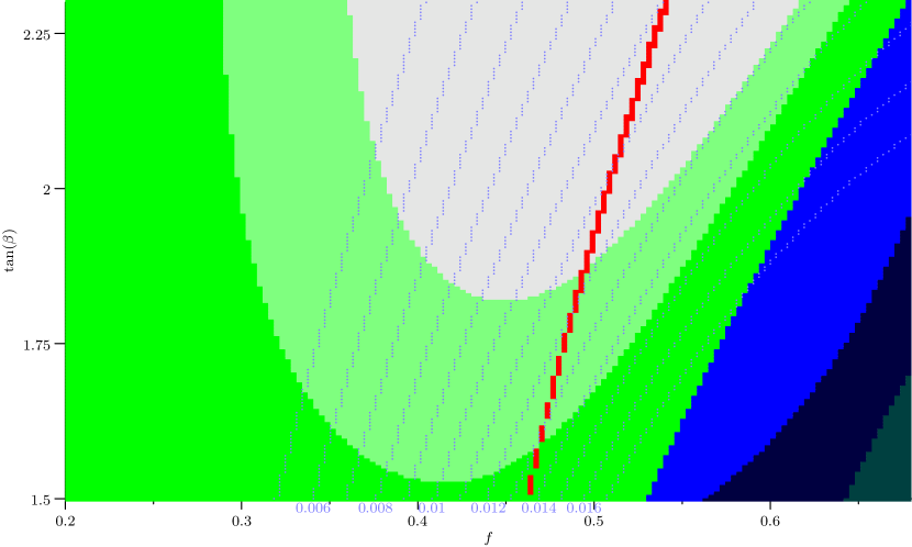
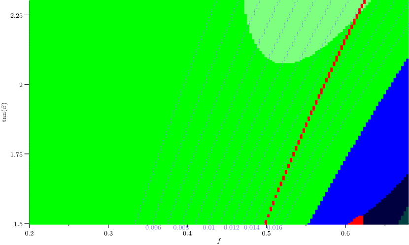
In order to construct benchmark scenarios that are consistent with cosmological observations and collider constraints we restrict our considerations to $\tan(\beta)\lesssim 2$. The plots in figure 6.1 show that in principle an appropriate value of the dark matter density can be obtained even when $\tan(\beta)>2$. However, larger values of $\tan(\beta)$ lead to the lightest and second lightest inert neutralinos having smaller masses as discussed in section 5.3. As a result larger couplings of the lightest inert neutralinos to the $Z$ boson are required to reproduce the measured value of $\Omega_{\mathrm{DM}}h^{2}$ and such light inert neutralinos with substantial couplings to $Z$ boson give a considerable contribution to its invisible width leading to a conflict with LEP measurements. This is discussed in more detail in the following subsection.

Even for $\tan(\beta)\lesssim 2$ the lightest inert neutralino states can get appreciable masses only if at least one of the inert chargino mass eigenstates is light $m_{\tilde{C}_{1}}\approx 100$–200 GeV. As clarified in sections 6.1 and 5.3, the masses of the lightest inert neutralino states decrease with increasing $m_{\tilde{C}_{1,2}}$ and it is therefore rather difficult to find benchmark scenarios consistent with cosmological observations for $m_{\tilde{C}_{1}}\gtrsim 200$ GeV. At the same time we demonstrate (with benchmark ix in table 6.3) that one light inert chargino mass eigenstate is enough to ensure that the lightest inert neutralino state gains a mass of order $m_{Z}/2$.

To obtain the kind of inert neutralino and chargino spectra discussed above one has to assume that the couplings $\lambda_{\alpha\beta}$ are rather small. They are expected to be much smaller than the largest $f_{d\alpha\beta}$ and $f_{u\alpha\beta}$ couplings. On the other hand, in order to get $|m_{\tilde{N}_{1}}|\sim|m_{\tilde{N}_{2}}|\sim m_{Z}/2$ the Yukawa couplings $f_{d\alpha\beta}$ and $f_{u\alpha\beta}$ need to be relatively close to their theoretical upper bounds caused by the requirement of the validity of perturbation theory up to the GUT scale. Since gauge coupling unification and RG flow determine the low energy value of $g^{\prime}_{1}$, the mass of the $Z_{2}$ gauge boson is approximately set by the SM-singlet VEV $s$ only. In our study we choose $s=2400$ GeV so that the $Z_{2}$ mass is about 890 GeV. This value of the $Z_{2}$ boson mass is just above the lower bound of 865 GeV found in ref. [67] — the most recent limit at the time of the publication of paper II — and allows satisfaction of stringent limits on the $Z_{2}$ mass and $Z$-$Z^{\prime}$ mixing that come from precision electroweak tests [69].

Since we restrict our analysis to low values of $\tan(\beta)\lesssim 2$ the mass of the SM-like Higgs boson is very sensitive to the choice of the coupling $\lambda$. Stringent LEP constraints require $\lambda$ at the EWSB scale to be larger than the low energy value of $g^{\prime}_{1}\approx 0.47$ and if one increases $\lambda$ much further then the theoretical upper bounds on $f_{d\alpha\beta}$ and $f_{u\alpha\beta}$ from RG running become substantially stronger. As a consequence, it is rather difficult to find solutions with $|m_{\tilde{N}_{1}}|\sim|m_{\tilde{N}_{2}}|\sim m_{Z}/2$. Therefore in our analysis we concentrate on values of $\lambda$ at the EWSB scale less than about 0.6. In addition we set stop SSB masses $m_{Q}=m_{u}=M_{s}=700$ GeV and restrict our consideration to the maximal mixing scenario with the stop mixing parameter, defined in (5.79), $X_{t}=\sqrt{6}M_{s}$. This choice of parameters limits the range of variations of the lightest $CP$-even Higgs mass. In the leading two-loop approximation the mass of the SM-like Higgs boson varies from 115 GeV for $\lambda=g^{\prime}_{1}$ to 136 GeV for $\lambda=0.6$. From tables 6.1, 6.2, and 6.3 one can see that the large values of $\lambda\gtrsim g^{\prime}_{1}$ that we choose in our analysis result in an extremely hierarchical Higgs spectrum, as pointed out in section 3.3. In tables 6.1, 6.2, and 6.3 the masses of the heavier Higgs states are computed in the leading one-loop approximation. In the case of the lightest Higgs boson mass the leading two-loop corrections are taken into account.

The set of benchmark points that we specify demonstrates that one can get a reasonable dark matter density consistent with recent observations if $|m_{\tilde{N}_{1}}|\sim|m_{\tilde{N}_{2}}|\sim m_{Z}/2$. Our benchmark scenarios also indicate that in this case the SM-like Higgs boson decays predominantly into the lightest inert neutralinos $\tilde{N}_{1}$ and $\tilde{N}_{2}$ while the total branching ratio into SM particles varies from 2% to 4%.

Benchmarks i, ii, iv, v, and viii are motivated by the non-Abelian flavour symmetry $\Delta_{27}$ which describes well the observed hierarchy in the quark and lepton sectors. As was discussed in subsection 6.1.2, these scenarios imply that all flavour diagonal Yukawa couplings $\lambda_{\alpha\alpha}$, $f_{d\alpha\alpha}$, and $f_{u\alpha\alpha}$ are rather small. Due to the approximate global $U(1)$ symmetry (6.14) that originates from the flavour symmetry $\Delta_{27}$, the spectrum of inert neutralinos comprises a set of pseudo-Dirac states. When the masses of the lightest and second lightest inert neutralinos are close, or they form an exact Dirac state, then the decays $h_{1}\rightarrow\tilde{N}_{\alpha}\tilde{N}_{\beta}$ lead to missing transverse energy in the final state. These decay channels give rise to a large invisible branching ratio for the SM-like Higgs boson.

In tables 6.1, 6.2, and 6.3 benchmarks i, ii, iv–vi, and ix have almost degenerate lightest and second lightest inert neutralinos. In some of these benchmark points both lightest inert neutralinos are lighter than $m_{Z}/2$ and as such the $Z$ boson can decay into $\tilde{N}_{\alpha}\tilde{N}_{\beta}$ so that the lightest and second lightest inert neutralino states contribute to the invisible $Z$ boson width. In other benchmark scenarios both of the lightest inert neutralinos have masses above $m_{Z}/2$ and the decays $Z\rightarrow\tilde{N}_{\alpha}\tilde{N}_{\beta}$ are kinematically forbidden.

When the LSP and NLSP are close in mass, LSP-NLSP coannihilation might be an important factor in determining the dark matter relic density. If this is the case then the LSP-NLSP mass splitting should be an important factor. Since annihilations of two identical neutralinos are p-wave suppressed, one should compare $\beta R_{Z11}$ with $R_{Z12}$ when trying to determine how important coannihilations are, where $\beta$ is the relative speed of the incoming particles, approximately 1/6 around the time of thermal freeze-out. It is useful to consider the following situations: With the LSP and NLSP almost degenerate and with equal self-annihilation cross-sections, but a negligible coannihilation cross-section, the relic density of dark matter would be twice what it would have have been if the NLSP had not been present. If, alternatively, the coannihilation cross-section was equal to the self-annihilation cross-sections then the existence of this extra channel would lead to a lower present day relic density. In this case it would in fact be equal to the relic density calculated in the absence of the NLSP. In this way, in such a scenario where coannihilations and self-annihilations are about as important as each other, the relic density actually ends up being largely independent of the LSP-NLSP mass splitting.

For the benchmarks i and ii this latter situation is approximately the case and the LSP-NLSP mass splitting turns out not to be an important factor. The mass splitting is in fact small — about half a GeV — but if it were larger and the NLSPs were made to have frozen-out much earlier, the relic density would only be decreased slightly (in this case by about a tenth). In benchmark iv, even though the LSP and NLSP are close in mass, coannihilations are unimportant due to the small value of $R_{Z12}$. In this case increasing the NLSP mass substantially while keeping everything else fixed would lead to an approximate halving of the predicted relic density, since the NLSP would have decoupled much earlier than, rather than at the same time as, the LSP. The only other benchmark scenario where the LSP and NLSP are close enough in mass for coannihilations to be potentially important is benchmark ix. Here coannihilation is in fact the dominant process and changing the LSP-NLSP mass splitting would have a large effect on the predicted relic density. In fact, in this scenario if the NLSP were not present the predicted relic density would be within the measured range.

If the mass difference between the second lightest and the lightest inert neutralino is around 10 GeV or more then some of the decay products of a $\tilde{N}_{2}$ that originates from a SM-like Higgs boson decay might be observed at the LHC. In our analysis we assume that all scalar particles, except for the lightest Higgs boson, are heavy and that the couplings of the inert neutralino states to quarks, leptons, and their superpartners are relatively small. As a result the second lightest inert neutralino decays into the lightest one and a fermion-antifermion pair mainly via a virtual $Z$. In our numerical analysis we did not manage to find any scenario with $|m_{\tilde{N}_{2}}|-|m_{\tilde{N}_{1}}|\gtrsim 20$ GeV leading to reasonable values of $\Omega_{\chi}h^{2}$. Hence we do not expect any observable jets at the LHC associated with the decay of a $\tilde{N}_{2}$ produced through a SM-like Higgs decay. However, it might be possible to detect some lepton-antilepton pairs coming from decays of the form $h_{1}\rightarrow\tilde{N}_{2}\tilde{N}_{\alpha}$. In particular we hope that $\mu^{+}\mu^{-}$ pairs coming from such decays of the lightest $CP$-even Higgs state could be observed at the LHC.

Benchmarks iii, vii, and viii can lead to such relatively energetic muon pairs in the final states of SM-like Higgs decays. Since the Higgs branching ratios into SM particles are rather suppressed, such decays of the lightest $CP$-even Higgs state might play an essential role in Higgs searches.

In addition to the inert Higgs decays, the scenarios considered here imply that at least two of the inert neutralino states that are predominantly formed from the fermionic components of the inert Higgs doublet supermultiplets, as well as one of the inert chargino states, should have masses below $200$ GeV. Since these states are almost inert Higgsinos they couple rather strongly to $W$ and $Z$ bosons. Thus at hadron colliders the corresponding inert neutralino and chargino states could be produced in pairs via off-shell $W$ and $Z$ bosons. Since they are light their production cross-sections at the LHC would not be negligibly small. After being produced, inert neutralino and chargino states would sequentially decay into the LSP and pairs of quarks and leptons resulting in distinct signatures that could be discovered at the LHC.

6.3.2 Neutralino and chargino collider limits

The remarkable signatures discussed above raise serious concerns that they could have already been observed at the Tevatron and/or even earlier at LEP. For example, the light inert neutralino and chargino states could have been produced at the Tevatron. The CDF and D0 collaborations have set a stringent lower bound on chargino masses using supersymmetry searches with a trilepton signal [119, 120]. These searches ruled out chargino masses below $164$ GeV. However, this lower bound on the chargino mass was obtained by assuming that the corresponding chargino and neutralino states decay predominantly into the LSP and a pair of leptons. In our case, however, the inert neutralino and chargino states are expected to decay via virtual $Z$ and $W$ exchange, decaying predominantly into the LSP and a pair of quarks. As a consequence the lower limit on the mass of charginos that is set by the Tevatron is not directly applicable to the benchmark scenarios that we consider here. Instead, in our study, we use the 95% confidence level lower limit on chargino masses of about $100$ GeV that was set by LEP [93].

In principle the LEP experiments also set constraints on the masses and couplings of neutral particles that interact with the $Z$ boson. As mentioned above, when the masses of $\tilde{N}_{1}$ and $\tilde{N}_{2}$ are below $m_{Z}/2$ they are almost degenerate and thus the decays of $Z\rightarrow\tilde{N}_{\alpha}\tilde{N}_{\beta}$ all contribute to the invisible width of the $Z$ boson, changing the effective number of neutrino species $N^{\mathrm{LEP}}_{{\mathrm{eff}}}$. The contribution of $\tilde{N}_{1}$ and $\tilde{N}_{2}$ to $N^{\mathrm{LEP}}_{{\mathrm{eff}}}$ is given by

$$\Delta N^{\mathrm{LEP}}_{{\mathrm{eff}}}=a_{11}+2a_{12}+a_{22},$$ (6.37)

where

$$a^{\vphantom{2}}_{\alpha\beta} = R_{Z\alpha\beta}^{2}\left[1-\dfrac{m_{\tilde{N}_{\alpha}}^{2}+m_{\tilde{N}_{\beta}}^{2}}{2m_{Z}^{2}}-3\dfrac{m_{\tilde{N}_{\alpha}}m_{\tilde{N}_{\beta}}}{m_{Z}^{2}}-\dfrac{\left(m_{\tilde{N}_{\alpha}}^{2}-m_{\tilde{N}_{\beta}}^{2}\right)^{2}}{2m_{Z}^{4}}\right]$$ (6.38)

$$\qquad\qquad\quad\sqrt{\left(1-\dfrac{m_{\tilde{N}_{\alpha}}^{2}+m_{\tilde{N}_{\beta}}^{2}}{m_{Z}^{2}}\right)^{2}-4\dfrac{m_{\tilde{N}_{\alpha}}^{2}m_{\tilde{N}_{\beta}}^{2}}{m_{Z}^{4}}}.$$

All three terms in (6.37) contribute to $\Delta N^{\mathrm{LEP}}_{{\mathrm{eff}}}$ only if $2|m_{\tilde{N}_{2}}|<m_{Z}$. In the case where only the $Z$ boson decays into $\tilde{N}_{1}\tilde{N}_{1}$ are kinematically allowed $a_{12}$ and $a_{22}$ should be set to zero. If $|m_{\tilde{N}_{1}}|+|m_{\tilde{N}_{2}}|<m_{Z}$ whilst $2|m_{\tilde{N}_{2}}|>m_{Z}$ then only $a_{11}$ and $2a_{12}$ contribute.

In order to compare the measured value of $N^{\mathrm{LEP}\,\smash{\mathrm{exp}}}_{{\mathrm{eff}}}$ with the effective number of neutrino species in the $E_{6}$SSM $N^{\mathrm{LEP}}_{{\mathrm{eff}}}=3+\Delta N^{\mathrm{LEP}}_{{\mathrm{eff}}}$ it is convenient to define the variable

$$D = \dfrac{N^{\mathrm{LEP}}_{{\mathrm{eff}}}-N^{\mathrm{LEP}\,\smash{\mathrm{exp}}}_{{\mathrm{eff}}}}{\sigma^{\mathrm{exp}}_{N^{\mathrm{LEP}}_{{\mathrm{eff}}}}}.$$ (6.39)

The value of $D$ represents the deviation between the predicted and measured effective number of neutrinos contributing to the $Z$ boson invisible width. It is worth pointing out that in the SM, from (1.23), $D=2$. In the benchmark scenarios presented in tables 6.1, 6.2, and 6.3 the value of $D$ is always less than 3. The plots in figure 6.1 also demonstrate that there is a substantial region of $E_{6}$SSM parameter space with $m_{\tilde{N}_{1,2}}<m_{Z}/2$ and $D<3$. This indicates that relatively light inert neutralinos with masses below $m_{Z}/2$ are not necessarily ruled out by constraints on the effective number of neutrinos set by LEP experiments. Indeed, as argued in section 6.1, the Yukawa couplings $f_{d\alpha\beta}$ and $f_{u\alpha\beta}$ can be chosen such that $R_{Z\alpha\beta}$ are very small. The couplings of the lightest and second lightest inert neutralinos to the $Z$ boson are relatively small anyway because of the inert singlino admixture in these states. Nevertheless, figure 6.1 shows that scenarios with light inert neutralinos having masses below $m_{Z}/2$ and relatively small couplings to the $Z$ boson can lead to appropriate dark matter densities consistent with observation.

LEP has set limits on the cross-sections of $e^{+}e^{-}\rightarrow\tilde{N}_{2}\tilde{N}_{1}$ and $e^{+}e^{-}\rightarrow\tilde{C}_{1}^{+}\tilde{C}_{1}^{-}$, where predominantly $\tilde{N}_{2}\rightarrow q\bar{q}\tilde{N}_{1}$ and $\tilde{C}_{1}\rightarrow q\bar{q}^{\prime}\tilde{N}_{1}$ respectively [121]. Unfortunately the bounds are not directly applicable for our study because OPAL limits were set for a relatively heavy $\tilde{N}_{2}$ or $\tilde{C}_{1}$ only — greater than about 60 GeV. Nevertheless, these bounds demonstrate that it was difficult to observe light neutralinos with masses less than about 100 GeV if their production cross-sections $\sigma(e^{+}e^{-}\rightarrow\tilde{N}_{\alpha}\tilde{N}_{\beta})\lesssim 0.1$–0.3 pb. Since at LEP energies the cross-sections of colourless particle production through s-channel $\gamma$/$Z$ exchange are typically a few picobarns, the lightest and second lightest inert neutralino states in the $E_{6}$SSM could have escaped detection at LEP if their couplings $R_{Z\alpha\beta}\lesssim 0.1$–0.3.

6.3.3 Dark matter direct detection

Another constraint on the couplings of the lightest inert neutralino comes from experiments for the direct detection of dark matter. At the time of the publication of paper II the most stringent upper limits on the DMP-nucleon elastic scattering spin-independent cross-section came from the CDMS collaboration [122] and from the first analysis of 11.7 days of data from the XENON100 experiment [123]. In the low DMP mass region relevant for our study, the most stringent of these was the XENON100 limit. In particular the XENON100 11.7 day analysis produced a limit on the cross-section of $3.4\times 10^{-44}$ cm² for a 55 GeV DMP at a confidence level of 90%. This limit remains fairly constant for lower DMP masses and does not increase above about $4\times 10^{-44}$ cm² for even the lowest LSP masses that are consistent with our thermal freeze-out scenario. Currently the most stringent limits on the spin-independent DMP-nucleon cross-section come from the more recent analysis of 100.9 days of data from XENON100 [124]. The best limit is $7.0\times 10^{-44}$ cm², which is for a 50 GeV DMP, again at a confidence level of 90%.

Since in the $E_{6}$SSM the couplings of the lightest inert neutralino to quarks, leptons, and their superpartners are suppressed, the spin-independent part of the $\tilde{N}_{1}$-nucleon elastic scattering cross-section is mediated mainly by t-channel SM-like Higgs boson exchange. Thus, in the leading approximation the spin-independent part of $\tilde{N}_{1}$-nucleon cross-section in the $E_{6}$SSM takes the form [125, 4]

$$\sigma_{\mathrm{SI}} = \dfrac{4m^{2}_{r}m_{N}^{2}}{\pi v^{2}m^{4}_{h_{1}}}|X^{h_{1}}_{11}F^{N}|^{2},$$ (6.40)

where $N$ is the nucleon,

$$m_{r} = \dfrac{m_{\tilde{N}_{1}}m_{N\vphantom{\tilde{N}_{1}}}}{m_{\tilde{N}_{1}}+m_{N\vphantom{\tilde{N}_{1}}}},\quad\mbox{and}$$

$$F^{N} = \sum_{q=u,d,s}f^{N}_{Tq}+\dfrac{2}{27}\sum_{Q=c,b,t}f^{N}_{TG},$$

with

$$m_{N}f^{N}_{Tq} = \langle N|m_{q}\bar{q}q|N\rangle\quad\mbox{and}$$

$$f^{N}_{TG} = 1-\sum_{q=u,d,s}f^{N}_{Tq}.$$

Here, for simplicity, we assume that the lightest Higgs state has the same couplings as a SM Higgs boson and ignore all contributions induced by heavy Higgs boson and squark exchange. Due to the hierarchical structure of the active Higgs boson spectrum and the approximate $\mathds{Z}^{H}_{2}$ symmetry this approximation works very well. Using the experimental limits set on $\sigma_{\mathrm{SI}}$ and (6.40) one can obtain upper bounds on $X^{h_{1}}_{11}$ [127].

In tables 6.1, 6.2, and 6.3 we specify the interval of variations of $\sigma_{\mathrm{SI}}$ for each benchmark scenario. As one can see from (6.40) the value of $\sigma_{\mathrm{SI}}$ depends rather strongly on the hadronic matrix elements — the coefficients $f^{N}_{Tq}$ that are related to the $\pi$-nucleon $\sigma$ term and the spin content of the nucleon. The hadronic uncertainties in the elastic scattering cross-section of DMPs and nucleons were considered in ref. [125]. In particular, it was pointed out that $f^{N}_{Ts}$ could vary over a wide range. In tables 6.1, 6.2, and 6.3 the lower limit on $\sigma_{\mathrm{SI}}$ corresponds to $f^{N}_{Ts}=0$ while the upper limit corresponds to $f^{N}_{Ts}=0.36$ (see ref. [4]). From tables 6.1, 6.2, and 6.3 and (6.40) it also becomes clear that $\sigma_{\mathrm{SI}}$ decreases substantially when $m_{h_{1}}$ grows.

Since in all of the benchmark scenarios presented in tables 6.1, 6.2, and 6.3 the lightest inert neutralino is relatively heavy, with $|m_{\tilde{N}_{1}}|\sim m_{Z}/2$, allowing for a small enough dark matter relic density, the coupling of $\tilde{N}_{1}$ to the lightest $CP$-even Higgs state is always large, giving rise to a $\tilde{N}_{1}$-nucleon spin-independent cross-section that is of the order of, or larger than, the 90% confidence level bound of ref. [123].

The dark matter scenario detailed in the present and previous chapters is now severely challenged by the most recent XENON100 results [124]. Although these results appear to rule out the $E_{6}$SSM as a model of dark matter, it should be noted that they do not rule out the model per se. Scenarios similar to those in tables 6.1 and 6.2, but in which the predicted relic density is somewhat less than the measured relic density can be consistent with direct detection experiments, although since such scenarios would not completely explain the observed dark matter relic density they may be considered less well motivated. In such scenarios it needs to be assumed that the majority of the observed dark matter is not composed of $E_{6}$SSM inert neutralino LSPs, but is composed of some extra matter beyond that of the $E_{6}$SSM.

6.4 Summary and Conclusions

In this work we considered novel decays of the SM-like Higgs boson in the $E_{6}$SSM. Particular attention was given to the dark matter that the model predicts and this work also represents a more in-depth study of the inert neutralino and chargino sectors of the $E_{6}$SSM than the previous study presented in chapter 5 and paper I.

To satisfy LEP constraints we restricted our consideration to scenarios with relatively heavy inert chargino states $m_{\tilde{C}_{1,2}}\gtrsim 100$ GeV. In our analysis we also required the validity of perturbation theory up to the GUT scale which sets stringent constraints on the values of the Yukawa couplings at low energies. Using these restrictions we argued that the lightest and the second lightest inert neutralinos are always light — they typically have masses below 60–65 GeV. These neutralinos are mixtures of inert Higgsinos and singlinos. In the considered model the lightest inert neutralino $\tilde{N}_{1}$ tends to be the LSP and play the role of dark matter while $\tilde{N}_{2}$ tends to be the NLSP. The masses of $\tilde{N}_{1}$ and $\tilde{N}_{2}$ decrease with increasing $\tan(\beta)>1$ and inert chargino masses.

Because the lightest inert neutralino states are predomiantly inert singlino in nature, their couplings to the gauge bosons, active Higgs bosons, quarks, and leptons are rather small, resulting in relatively small LSP annihilation cross-sections and the possibility of an unacceptably large dark matter density. In the limit where all non-SM states except for the inert neutralinos and charginos are heavy a reasonable density of dark matter can be obtained if $|m_{\tilde{N}_{1,2}}|\sim m_{Z}/2$, where the inert LSPs annihilate mainly through an s-channel $Z$ boson. On resonance an appropriate value of $\Omega_{\chi}h^{2}$ can be achieved even for a relatively small coupling of the LSP to the $Z$ boson. In order to achieve plausible scenarios consistent with both LEP and cosmological observations, requiring $|m_{\tilde{N}_{1}}|\sim m_{Z}/2$ if $\tilde{N}_{1}$ contributes to CDM, $\tan(\beta)$ cannot be too large.

The main message arising from this work is that within the dark matter motivated scenario although the lightest and the second lightest inert neutralinos can have small couplings to the $Z$ boson their couplings to the SM-like Higgs state $h_{1}$ are always large. Indeed, we argued that in the first approximation the couplings of $\tilde{N}_{1}$ and $\tilde{N}_{2}$ to the lightest $CP$-even Higgs boson are proportional to $|m_{\tilde{N}_{1}}|/v$ and $|m_{\tilde{N}_{2}}|/v$ respectively. Since $|m_{\tilde{N}_{1,2}}|$ must be of order $m_{Z}/2$ in order for the theory not to predict too much dark matter, these couplings are much larger than the corresponding coupling of $b$ quarks to the SM-like Higgs boson. Thus the SM-like Higgs boson decays predominantly into the lightest inert neutralino states and has very small branching ratios (2%–4%) for decays into SM particles.

The most recent XENON100 dark matter direct detection limits [124] now place rather stringent constraints on the $E_{6}$SSM inert neutralino dark matter scenario. As an explanation for all of the observed dark matter relic density the model now looks to be ruled out. There do, however, exist scenarios in which the $E_{6}$SSM LSP accounts for only some fraction of the observed dark matter that are consistent with constraints from colliders and cosmology.

Chapter 7 Dark Matter and Big Bang Nucleosynthesis in the $E_{6}\mathds{Z}^{S}_{2}$SSM

In this chapter, which contains work that was first published in paper III, with the exception of section 7.5 which contains work that is original to this thesis, we introduce a new scenario for dark matter in the $E_{6}$SSM in which the dark matter candidate is just the usual bino. At first sight having a bino dark matter candidate seems impossible since, as already discussed, the lightest inert neutralino mass eigenstates, predominantly the inert singlinos $\tilde{S}_{\alpha}$, naturally have suppressed masses and it is very difficult to make them even as heavy as half the $Z$ mass. To overcome this we propose that the inert singlinos are exactly massless and decoupled from the bino, which is achieved in practice by setting the Yukawa couplings $f_{(d,u)\alpha\beta}$ to zero. This is easy to do by introducing a discrete symmetry $\mathds{Z}^{S}_{2}$ under which the inert singlet scalars $S_{\alpha}$ are odd and all other bosonic states are even — a scenario we refer to as the $E_{6}\mathds{Z}^{S}_{2}$SSM.

In the $E_{6}\mathds{Z}^{S}_{2}$SSM the inert singlinos $\tilde{S}_{\alpha}$ will be denoted as $\tilde{\sigma}$ in order to emphasise their different (massless and decoupled) nature. The stable DMP is then generally mostly bino and the observed dark matter relic density can be achieved via a novel scenario in which the bino inelastically scatters off of SM matter into heavier inert Higgsinos during the time of thermal freeze-out, keeping the bino in equilibrium long enough to give the desired relic abundance. As long as the inert Higgsinos are close in mass to the bino this is always possible to arrange — the only constraint being that the inert Higgsinos satisfy the LEP constraint of being heavier than 100 GeV. This in turn implies that the bino must also be heavier than or close to 100 GeV. These constraints are easy to satisfy and, unlike in the inert neutralino LSP dark matter scenario, we find that successful relic abundance can be achieved within a GUT scale constrained version of the model — the c$E_{6}\mathds{Z}^{S}_{2}$SSM — assuming a unified soft scalar mass $m_{0}$, soft gaugino mass $M_{1/2}$, and soft trilinear mass $A_{0}$ at the GUT scale.

It is worth noting that studies of the c$E_{6}$SSM [128, 5, 65] have hitherto neglected to study the full $12\times 12$ neutralino mass matrix and only considered the $6\times 6$ mass matrix of the USSM [4]. Although the question of dark matter was addressed in the USSM, the requirement of successful relic abundance was not imposed on the c$E_{6}$SSM in refs. [128, 5, 65] even though both analyses considered the same $6\times 6$ neutralino mass matrix. This is because it was expected that dark matter would arise from the inert sector of the c$E_{6}$SSM which was not studied. When cosmological constraints on inert neutralino dark matter are included in the $E_{6}$SSM certain trilinear Higgs Yukawa couplings relevant to the inert sector are required to be large as we saw in chapters 5 and 6. In the c$E_{6}$SSM these large couplings strongly affect the RG running from the GUT scale and we have not been able to show that having inert neutralino LSPs consistent with CDM constraints can also be consistent with having universal (GUT scale constrained) soft mass parameters. Here we shall consider the c$E_{6}$SSM with the full $12\times 12$ neutralino mass matrix, including both the USSM and inert neutralinos, under the assumption that the fermionic components of the inert SM-singlet supermultiplets, the two inert singlinos, are forbidden to acquire mass by an extra $\mathds{Z}_{2}$ symmetry of the superpotential. In practice there is then a $10\times 10$ neutralino mass matrix once the two massless inert singlinos are decoupled.

In summary, the main result of this study is that bino dark matter, with nearby inert Higgsinos and massless inert singlinos, provides a simple and consistent picture of dark matter in the $E_{6}$SSM and is consistent with GUT scale unified soft parameters. We also consider the effect of the presence of the two massless inert singlinos in the $E_{6}\mathds{Z}^{S}_{2}$SSM on the effective number of neutrinos contributing to the expansion rate of the universe prior to BBN, affecting ⁴He production. Current fits to WMAP data [129] favour values greater than three, so the presence of additional contributions to the effective number of neutrinos is another interesting aspect of the $E_{6}\mathds{Z}^{S}_{2}$SSM. In practice we find that the additional number of effective neutrino species is less than two, due to entropy dilution, depending on the mass of the $Z^{\prime}$ boson which keeps the inert singlinos in equilibrium.

The $E_{6}\mathds{Z}^{S}_{2}$SSM is introduced and its neutralino sector is explored in section 7.1. The details of the dark matter calculation are presented in section 7.2. $N_{{\mathrm{eff}}}$ is defined and calculations of its value in the $E_{6}\mathds{Z}^{S}_{2}$SSM are presented in section 7.3. Some benchmark points are presented in section 7.4. The possibility of inert singlino WDM is discussed in section 7.5 and the conclusions are summarised in section 7.6.

7.1 The $E_{6}\mathds{Z}^{S}_{2}$SSM

In the $E_{6}\mathds{Z}^{S}_{2}$SSM, as well as being invariant under $\mathds{Z}^{M}_{2}$ and either $\mathds{Z}^{L}_{2}$ or $\mathds{Z}^{B}_{2}$, summarised in tables 3.2 and 7.1, the superpotential of the $E_{6}$SSM (3.6) is also invariant under an additional exact $\mathds{Z}_{2}$ symmetry called $\mathds{Z}^{S}_{2}$. Under this symmetry only the two inert SM-singlet fields $S_{\alpha}$ are odd. The couplings of the forms $\lambda_{\alpha ij}$ and $\kappa_{\alpha ij}$ are therefore forbidden. This means that the fermionic superpartners of $S_{\alpha}$ — the inert singlinos $\tilde{\sigma}$ — are forbidden to have mass and do not mix with the other neutralinos. They interact only via their gauge couplings to the $Z^{\prime}$ boson which exist since they are charged under the $U(1)_{N}$ gauge symmetry.

All of the exact and approximate discrete symmetries relevant to the $E_{6}\mathds{Z}^{S}_{2}$SSM superpotential are summarised in table 7.1.

	$\mathds{Z}^{M}_{2}$	$\mathds{Z}^{L}_{2}$	$\mathds{Z}^{B}_{2}$	$\mathds{Z}^{H}_{2}$	$\mathds{Z}^{S}_{2}$
$S^{\vphantom{c}}_{\alpha}$	$+$	$+$	$+$	$-$	$-$
$H^{\vphantom{c}}_{d\alpha},H^{\vphantom{c}}_{u\alpha}$	$+$	$+$	$+$	$-$	$+$
$S^{\vphantom{c}}_{3},H^{\vphantom{c}}_{d3},H^{\vphantom{c}}_{u3}$	$+$	$+$	$+$	$+$	$+$
$\tilde{Q}^{\vphantom{c}}_{Li},\tilde{d}^{c}_{Ri},\tilde{u}^{c}_{Ri}$	$-$	$+$	$+$	$-$	$+$
$\tilde{L}^{\vphantom{c}}_{Li},\tilde{e}^{c}_{Ri},\tilde{N}^{c}_{i}$	$-$	$-$	$-$	$-$	$+$
$\bar{D}^{\vphantom{c}}_{i},D^{\vphantom{c}}_{i}$	$+$	$+$	$-$	$-$	$+$

Table 7.1: The charges of the fields of the $E_{6}\mathds{Z}^{S}_{2}$SSM superpotential under various exact and approximate $\mathds{Z}_{2}$ symmetries that the superpotential may or may not obey. $\mathds{Z}^{M}_{2}$ is already a symmetry due to gauge invariance. Either $\mathds{Z}^{L}_{2}$ or $\mathds{Z}^{B}_{2}$ is imposed in order to avoid rapid proton decay. $\mathds{Z}^{H}_{2}$ is an approximate flavour symmetry. In the $E_{6}\mathds{Z}^{S}_{2}$SSM the extra symmetry $\mathds{Z}^{S}_{2}$ is imposed, forcing the inert singlinos to be massless and decoupled. $i\in\{1,2,3\}$ and $\alpha\in\{1,2\}$.

One may worry that the effects of the massless inert singlinos would have already been seen in precision measurements from LEP. The inert singlinos, although not mixing with the inert Higgsinos as they did in the $E_{6}$SSM inert neutralino dark matter scenario, still couple to the $Z_{1}$ mass eigenstate because of the non-zero $Z$-$Z^{\prime}$ mixing angle $\alpha_{ZZ^{\prime}}$ defined in (3.23). In the following we neglect the kinetic term mixing that is expected to be a small effect (see section 3.2). For a given $m_{Z^{\prime}}\approx m_{\vphantom{Z^{\prime}}Z_{2}}$ in (3.21) $m^{2}_{ZZ^{\prime}}$, and hence also $\alpha_{ZZ^{\prime}}$, is maximised in the limit $\tan(\beta)\rightarrow\infty$. For $m_{Z_{2}}\approx m_{Z^{\prime}}=892$ GeV the maximum value of $m^{2}_{ZZ^{\prime}}$ is 3270 GeV² and the maximum value of $\alpha_{ZZ^{\prime}}$ is then $4.15\times 10^{-3}$. The $Z_{1}$-$\tilde{\sigma}$-$\tilde{\sigma}$ coupling relative to the $Z$-$\nu$-$\nu$ gauge coupling $R$ is equal to $\alpha_{ZZ^{\prime}}$. From (6.37) the change in the effective number of neutrinos contributing to the invisible $Z$ boson width at LEP due to the presence of massless inert singlinos is then $\Delta N^{\mathrm{LEP}}_{{\mathrm{eff}}}=2R^{2}=2\alpha^{2}_{ZZ^{\prime}}=1.72\times 10^{-5}$ which is well below the experimental uncertainty $\sigma^{\mathrm{exp}}_{N^{\mathrm{LEP}}_{{\mathrm{eff}}}}=8\times 10^{-3}$. When the $Z_{2}$ boson mass is large enough to avoid experimental detection limits the contributions of massless inert singlinos to the $Z$ boson width and to other LEP precision measurements are expected to be within the experimental error.

7.1.1 The neutralinos of the $E_{6}\mathds{Z}^{S}_{2}$SSM

The chargino sector of the $E_{6}\mathds{Z}^{S}_{2}$SSM is unchanged from that of the $E_{6}$SSM without $\mathds{Z}^{S}_{2}$. The chargino mass matrix is that given in (5.47). The same is true for the active Higgs scalar masses and mass matrices given in section 3.3. The situation in the neutralino sector, however, is quite different.

In the present study of the $E_{6}\mathds{Z}^{S}_{2}$SSM we define the term ‘neutralino’ not to include the massless inert singlinos which do not appear in the superpotential and are decoupled. The neutralino mass matrix $M^{N}$ in the interaction basis

$$\tilde{N}_{\mathrm{int}} = \left(\begin{array}[]{cccccc|cc}\tilde{B}&\tilde{W}^{3}&\tilde{H}^{0}_{d3}&\tilde{H}^{0}_{u3}&\tilde{S}^{\vphantom{0}}_{3}&\tilde{B}^{\prime}&\tilde{H}^{0}_{d\alpha}&\tilde{H}^{0}_{u\beta}\end{array}\right)^{T},$$ (7.2)

and again neglecting the small bino-bino^′ mixing, is then equal to

$$\left(\begin{array}[]{cccccc|cc}M^{\vphantom{\prime}}_{1}&0&-\frac{1}{2}g^{\prime}v_{d}&\frac{1}{2}g^{\prime}v_{u}&0&0&0&0\\ 0&M^{\vphantom{\prime}}_{2}&\frac{1}{2}gv_{d}&-\frac{1}{2}gv_{u}&0&0&0&0\\ -\frac{1}{2}g^{\prime}v_{d}&\frac{1}{2}gv_{d}&0&-\mu&-\frac{\lambda_{333}v_{u}}{\sqrt{2}}&Q^{N}_{d}g_{1}^{\prime}v_{d}&0&-\frac{\lambda_{33\beta}s}{\sqrt{2}}\\ \frac{1}{2}g^{\prime}v_{u}&-\frac{1}{2}gv_{u}&-\mu&0&-\frac{\lambda_{333}v_{d}}{\sqrt{2}}&Q^{N}_{u}g_{1}^{\prime}v_{u}&-\frac{\lambda_{3\alpha 3}s}{\sqrt{2}}&0\\ 0&0&-\frac{\lambda_{333}v_{u}}{\sqrt{2}}&-\frac{\lambda_{333}v_{d}}{\sqrt{2}}&0&Q^{N}_{S}g_{1}^{\prime}s&-\frac{\lambda_{3\alpha 3}v_{u}}{\sqrt{2}}&-\frac{\lambda_{33\beta}v_{d}}{\sqrt{2}}\\ 0&0&Q^{N}_{d}g_{1}^{\prime}v_{d}&Q^{N}_{u}g_{1}^{\prime}v_{u}&Q^{N}_{S}g_{1}^{\prime}s&M^{\prime}_{1}&0&0\\ \hline\cr 0&0&0&-\frac{\lambda_{3\alpha 3}s}{\sqrt{2}}&-\frac{\lambda_{3\alpha 3}v_{u}}{\sqrt{2}}&0&0&-\frac{\lambda_{3\alpha\beta}s}{\sqrt{2}}\\ 0&0&-\frac{\lambda_{33\beta}s}{\sqrt{2}}&0&-\frac{\lambda_{33\beta}v_{d}}{\sqrt{2}}&0&-\frac{\lambda_{3\alpha\beta}s}{\sqrt{2}}&0\end{array}\right),$$ (7.11)

(7.12)

where once again $Q^{N}_{d,u,S}$ are the $U(1)_{N}$ charges of down-type Higgsinos, up-type Higgsinos, and singlinos respectively, as given in table 3.1. Typically $g^{\prime}_{1}\approx g^{\vphantom{\prime}}_{1}$ all the way down to the low energy scale. If the soft gaugino masses are unified at the GUT scale then we also have $M^{\prime}_{1}\approx M^{\vphantom{\prime}}_{1}\approx M^{\vphantom{\prime}}_{2}/2$ (see subsection 3.2.1).

The Yukawa couplings in the off-diagonal blocks, marked out by lines, are suppressed under the approximate $\mathds{Z}_{2}^{H}$. Given the smallness of these couplings, the inert neutralinos in the bottom-right block are pseudo-Dirac states with an approximately decoupled mass matrix

$$-\frac{s}{\sqrt{2}}\left(\begin{array}[]{cccc}&&\lambda_{322}&\lambda_{321}\\ &&\lambda_{312}&\lambda_{311}\\ \lambda_{322}&\lambda_{312}&&\\ \lambda_{321}&\lambda_{311}&&\end{array}\right) \left(\begin{array}[]{cccc}\tilde{H}^{0}_{d2}&\tilde{H}^{0}_{d1}&\tilde{H}^{0}_{u2}&\tilde{H}^{0}_{u1}\end{array}\right)^{\mathrm{T}}.$$ in the basis (7.18)

They are approximately degenerate with the two inert chargino Dirac states.

The top-left block is the USSM neutralino mass matrix (5.10) and contains the states of the MSSM supplemented by the third generation singlino and the bino^′. In the case where $M^{\vphantom{\prime}}_{1}\approx M^{\prime}_{1}$ is small the lightest neutralino mass state will be mostly bino. The bino^′ will mix with the third generation singlino giving two mixed states with masses around $Q^{N}_{S}g_{1}^{\prime}s$. As $M_{1}\approx M_{1}^{\prime}$ increases, the bino mass will increase relative to both the third generation Higgsino mass $\mu$ and the inert Higgsino masses given approximately by the biunitary diagonalisation of

$$-\dfrac{1}{\sqrt{2}}\lambda_{3\alpha\beta}s.$$

At the same time the state mostly containing the third generation singlino will have a decreasing mass as $M_{1}^{\prime}$ increases relative to $Q^{N}_{S}g_{1}^{\prime}s$.

7.2 Dark Matter in the c$E_{6}\mathds{Z}^{S}_{2}$SSM

As discussed previously, in section 3.1, there is an automatically conserved $R$-parity under which the charginos, neutralinos, inert singlinos $\tilde{\sigma}$, and exotic $\tilde{\bar{D}}$ and $\tilde{D}$ fermions, along with the squarks and sleptons, are all $R$-parity odd, i.e. all of the fermions other than the quarks and leptons are $R$-parity odd. We shall assume that the lightest neutralino $\tilde{N}_{1}$ is the lightest of all of the $R$-parity odd states excluding the massless inert singlinos $\tilde{\sigma}$. However, $\tilde{N}_{1}$ cannot decay into $\tilde{\sigma}$ via neutralino mixing since the inert singlinos are decoupled from the neutralino mass matrix. Furthermore, the potential decay $\tilde{N}_{1}\rightarrow\tilde{\sigma}\sigma$, allowed by the $\sigma$-$\tilde{\sigma}$-$\tilde{B}^{\prime}$ supersymmetric $U(1)_{N}$ gauge coupling, is forbidden if $\tilde{N}_{1}$ is lighter than the inert SM-singlet scalars $\sigma$. In fact, in this case no kinematically viable final states exist that have the same quantum numbers as $\tilde{N}_{1}$. Therefore $\tilde{N}_{1}$ is absolutely stable and in the scenario presented is the DMP. The lightest inert SM-singlet scalar is not stable. There are no Yukawa couplings involving $S_{\alpha}$, but the inert SM-singlet scalars are able to decay via the $\sigma$-$\tilde{\sigma}$-$\tilde{B}^{\prime}$ supersymmetric $U(1)_{N}$ gauge coupling.

In the successful dark matter scenario presented in this section $\tilde{N}_{1}$ is predominantly bino, with at least one of the two pairs of pseudo-Dirac inert Higgsinos expected to be close in mass, but somewhat heavier, in order to achieve the correct relic density. This is due to a novel scenario in which the DMP is approximately the bino and inelastically scatters off of SM matter into heavier inert Higgsinos during the time of thermal freeze-out, keeping it in equilibrium long enough to give a successful relic density. In this section we discuss in detail how this novel scenario comes about in this model.

7.2.1 The dark matter calculation

In the considered model the DMP is not the lightest $R$-parity odd state — an inert singlino — but the lightest neutralino $\tilde{N}_{1}$. We would like to use (4.3) to describe the evolution of $R$-parity odd states other than the inert singlinos — generically $\tilde{\chi}$. In this case we should also include in (4.3) processes involving $\sigma$ and $\tilde{\sigma}$ particles that change the number of $\tilde{\chi}$ particles by one. Since such processes necessarily involve inert SM-singlet scalars $\sigma$, it is valid to neglect these processes in the case where these inert SM-singlet bosons have frozen out long before the freeze-out of dark matter. We will call this condition B, to go along with condition A, defined in subsection 4.1, and it should be satisfied given our assumption that the inert SM-singlet scalar mass eigenstates are heavier than the DMP, since they only interact via the heavy $Z^{\prime}$ boson. Assuming that both conditions A and B are satisfied we can use (4.6) to describe the evolution of the number density $n$ of $R$-parity-odd states other than inert singlinos $\tilde{\chi}$. The value of $n$ after the thermal freeze-out of $\tilde{N}_{1}$ depends on annihilation cross-sections involving $\tilde{N}_{1}$ and other $R$-parity odd states close by in mass and $n$ will eventually be equal to the number density of DMPs after other $\tilde{\chi}$ states have decayed to $\tilde{N}_{1}$.

7.2.2 The c$E_{6}\mathds{Z}^{S}_{2}$SSM dark matter scenario

In order to carry out the dark matter analysis in the constrained version of the model we have extended the RG code used for the study in ref. [5] [130] to include the Yukawa parameters and soft masses of the inert sector of the $E_{6}\mathds{Z}^{S}_{2}$SSM. The inputs are $\kappa_{3ij}$ and $\lambda_{333}$ at the GUT scale, $\lambda_{3\alpha\beta}$ at the EWSB scale, $s$, and $\tan(\beta)$, as well as the known low energy Yukawa couplings and gauge couplings. Given these inputs and the RGEs the algorithm attempts to find points with GUT scale unified soft masses $m_{0}$, $M_{1/2}$, and $A_{0}$. The low energy $U(1)_{N}$ gauge coupling $g_{1}^{\prime}$ is set by requiring it to be equal to the other gauge couplings at the GUT scale, which is calculated.

For consistent points in the $E_{6}$SSM the lightest non-inert (USSM sector) supersymmetric particle is typically bino dominated. For the c$E_{6}\mathds{Z}^{S}_{2}$SSM we find the same thing. The masses of the inert Higgsino states depend on $s$ and on the Yukawa couplings $\lambda_{3\alpha\beta}$ and in the c$E_{6}\mathds{Z}^{S}_{2}$SSM the lightest neutralino can be either the bino dominated state or a pseudo-Dirac inert Higgsino dominated state. In the latter case we find that the pseudo-Dirac inert Higgsino DMPs coannihilate with full-weak-strength interactions and lead to a too small dark matter relic density. In the former case the bino DMP normally annihilates too weakly and yields a too large dark matter relic density. If, however, there are inert Higgsino states close by in mass, they contribute significantly to $\langle\sigma v\rangle$, allowing for the observed amount of dark matter. This relies on condition A being satisfied, i.e. the binos being up-scattered into inert Higgsinos at a large enough rate.

Such points with an appropriate dark matter relic density can be found and three are presented in section 7.4. Condition B is satisfied since the inert SM-singlet scalars are so much heavier than the DMP and the $Z_{2}$ boson mass is so large compared to the regular $Z$ boson mass. Annihilation and scattering processes involving inert SM-singlets and singlinos must contain a virtual $Z^{\prime}$ boson, which is predominantly the $Z_{2}$ mass eigenstate.

To test condition A let us compare the rate for binos up-scattering into inert Higgsinos with the inert Higgsino coannihilation rate. We shall label the mostly bino state $\tilde{N}_{1}$ and the lightest pseudo-Dirac inert Higgsino states $\tilde{N}_{2}$ and $\tilde{N}_{3}$. The dominant up-scattering diagrams are of the form shown in figure 7.1.

Figure 7.1: The form of diagrams for the up-scattering of the bino dominated DMP $\tilde{N}_{1}$ off of SM particles $X$ into the pseudo-Dirac inert Higgsino states $\tilde{N}_{2}$ and $\tilde{N}_{3}$.

As in section 6.1 we again define $R_{Zij}$ couplings such that the $Z$-$\tilde{N}_{i}$-$\tilde{N}_{j}$ coupling is equal to $R_{Zij}$ times the $Z$-$\nu$-$\nu$ coupling. In the $E_{6}\mathds{Z}^{S}_{2}$SSM we can write

$$R_{Zij} = \sum_{D=3,7,9}N_{i}^{D}N_{j}^{D}-\sum_{U=4,8,10}N_{i}^{U}N_{j}^{U},$$ (7.19)

where $N_{i}^{a}$ is the neutralino mixing matrix element corresponding to mass eigenstate $i$ and interaction state $a$. $D$ and $U$ index the down- and up-type Higgsino interaction states respectively. For the pseudo-Dirac inert Higgsino states we have $m_{3}\approx-m_{2}$ and $R_{Z23}\approx 1$, allowing for full-weak-strength coannihilations of the form shown in figure 7.2.

Figure 7.2: Full-weak-strength coannihilations of the pseudo-Dirac inert Higgsino states $\tilde{N}_{2}$ and $\tilde{N}_{3}$.

Using the notation from (4.3), the ratio of the rate for the mostly bino state up-scattering into the lightest mostly inert Higgsino state to the inert Higgsino coannihilation rate is given approximately by

$$\Upsilon = \frac{\langle\sigma^{\prime}_{X12}v^{\vphantom{\prime}}_{1X}\rangle n_{1}^{\mathrm{eq}}n_{X}^{\mathrm{eq}}}{\langle\sigma^{\vphantom{\prime}}_{23}v^{\vphantom{\prime}}_{23}\rangle n_{2}^{\mathrm{eq}}n_{3}^{\mathrm{eq}}}.$$ (7.20)

To give an idea of the size of this ratio, if the SM particle $X$ is relativistic and $m_{1}\sim m_{2}\approx m_{3}$ then

$$\Upsilon \sim \left(\frac{R_{Z12}}{R_{Z23}}\right)^{2}\frac{T^{3}}{(|m_{1}|T)^{3/2}\exp(-|m_{1}|/T)}$$ (7.21)

$$\approx R_{Z12}^{2}x^{3/2}e^{-x},$$

where again

$$x=\dfrac{T}{|m_{1}|}.$$

This ratio is expected to be large because of the overwhelming abundance of the relativistic SM particle $X$, but it also depends on $R_{Z12}$. The value of $R_{Z12}$ depends on the $\mathds{Z}^{H}_{2}$-breaking couplings that mix the upper-left block of the neutralino mass matrix in (7.12) — the USSM states including the bino — with the inert Higgsino states in the lower-right block. Since this symmetry is not exact we expect these couplings to be large enough such that we can still assume $\Upsilon\gg 1$. Explicit examples of this parameter are included in table 7.3 in section 7.4.

With conditions A and B satisfied we use micrOMEGAs [91] to calculate the dark matter relic density for low energy spectra consistent with the GUT scale constrained scenario. The observed relic density of dark matter can arise in this model and examples are shown in table 7.3 in section 7.4. The most critical factor is the mass splitting between the bino and the lightest inert Higgsinos. Too large and there are not enough inert Higgsinos remaining at the time of the bino’s thermal freeze-out to have a significant enough effect. Too small and $\langle\sigma v\rangle$ is dominated by inert Higgsino coannihilations, leading to a too small dark matter relic density.

Since in this scenario the DMP is predominantly bino, the spin-independent DMP-nucleon cross-section $\sigma_{\mathrm{SI}}$ is not expected to be in the range that direct detection experiments are currently sensitive too. The spin-independent cross-section of a pure bino is suppressed by the squark masses, but is also sensitive to the squark mixing angles [131]. For each flavour the cross-section vanishes for zero squark mixing. Since in practice the DMP will also have non-zero, but small, active Higgsino components, there are also contributions to $\sigma_{\mathrm{SI}}$ from t-channel active Higgs scalar exchange via the bino-Higgs-Higgsino supersymmetric gauge coupling. These contributions, though in fact dominant, are quite small, due to the overwhelming bino nature of the DMP. Estimates of $\sigma_{\mathrm{SI}}$, using the same proton $f_{d}$, $f_{u}$, and $f_{s}$ parameters used in the study in ref. [132], are included in table 7.3 in section 7.4.

7.3 The Inert Singlinos and their Contribution to the Effective Number of Neutrinos prior to BBN

In the standard theory of BBN, which happens long after the thermal freeze-out of dark matter, the resultant primordial abundances of the light elements depend on two parameters — the effective number of neutrinos contributing to the expansion rate of the radiation dominated universe $N_{{\mathrm{eff}}}$ and the baryon-to-photon ratio $\eta$.

Whilst the primordial abundance of ⁴He is not the most sensitive measure of $\eta$, it is much more sensitive to $N_{{\mathrm{eff}}}$ than the other light element abundances. This is because prior to nucleosynthesis, when the equilibrium photon temperature is of order 0.1 MeV, the number of neutrons remaining, virtually all of which are subsequently incorporated into ⁴He nuclei, is sensitive to the expansion rate of the universe, which depends on $N_{{\mathrm{eff}}}$. The greater the expansion rate, the less time there is for charged current weak interactions to convert neutrons into protons.

The analysis in ref. [133], using the more recent neutron lifetime measurement from ref. [134], gives $N_{{\mathrm{eff}}}=3.80^{+0.80}_{-0.70}$ at 2-sigma, implying a more-than-2-sigma tension between the measured ⁴He abundance and the Standard Model prediction for $N_{{\mathrm{eff}}}$ of about 3. Although in ref. [135] it is suggested that these errors may be larger, similar results are also obtained for the effective number of neutrinos contributing to the expansion rate of the universe from fits to WMAP data [129].

In the $E_{6}\mathds{Z}^{S}_{2}$SSM the two massless inert singlinos would have decoupled from equilibrium at an earlier time than the light neutrinos, but nevertheless would have contributed to $N_{{\mathrm{eff}}}$. Exactly when the inert singlinos would have decoupled from equilibrium with the photon depends on the mass of the $Z_{2}$ boson which determines the strength of an effective Fermi-like 4-point interaction vertex that would have been responsible for keeping the inert singlinos in equilibrium. The various values for $N_{{\mathrm{eff}}}$ that can be achieved in this model all fit the data better than the SM value.

The implications of extra neutrino-like particles present in the early universe have long been studied and the methods used in following analysis rely on relatively simple physics (see for example ref. [136]).

The effective number of degrees of freedom contributing to the expansion rate of the universe during the run-up to nucleosynthesis is defined by

$$g_{\mathrm{eff}}^{0} = g_{\gamma}+\nicefrac{{7}}{{8}}g_{\nu}N_{{\mathrm{eff}}}(\nicefrac{{4}}{{11}})^{4/3}$$ (7.22)

$$= 2+\nicefrac{{7}}{{4}}N_{{\mathrm{eff}}}(\nicefrac{{4}}{{11}})^{4/3},$$

where $g_{\mathrm{eff}}^{0}$ is the value of $g^{\vphantom{0}}_{{\mathrm{eff}}}$, as defined in (4.9), immediately prior to nucleosynthesis. Here $g_{\gamma}=2$ is the number of degrees of freedom of the photon and $g_{\nu}=2$ is the number of degrees of freedom of a light neutrino. The three SM neutrinos are expected to decouple from equilibrium with the photon at a temperature above the electron mass whereas nucleosynthesis does not happen until the temperature is below the electron mass. When the photon/electron temperature is around the electron mass the electrons and positrons effectively disappear from the universe. Their disappearance heats the photons to a higher temperature then they would otherwise have had, but the neutrinos, having already decoupled, would continue to cool at the full rate dictated by Hubble expansion. Because of the neutrinos’ lower temperature at nucleosynthesis they would then contribute less to $g_{\mathrm{eff}}^{0}$ per degree of freedom. In (7.22) $N_{{\mathrm{eff}}}$ is defined such that in the SM $N_{{\mathrm{eff}}}=3$, for the three neutrinos decoupling above the electron mass, as we shall see. Extra particles, such as the $E_{6}\mathds{Z}^{S}_{2}$SSM inert singlinos, decoupling above the muon mass would have had even lower temperatures at the time of nucleosynthesis and would therefore contribute to $g_{\mathrm{eff}}^{0}$ even less than light neutrinos per degree of freedom.

7.3.1 The calculation of $N_{{\mathrm{eff}}}$

In the c$E_{6}\mathds{Z}^{S}_{2}$SSM there is a typical scenario in which the massless inert singlinos $\tilde{\sigma}$ decouple at a temperature above the colour transition temperature (when the effective degrees of freedom are quarks and gluons rather than mesons) and above the strange quark mass, but below the charm quark mass. This has to do with the strength of the interactions that keep the inert singlinos in equilibrium which depend heavily on the mass of the $Z_{2}$ boson. If the inert singlinos do decouple in this range then this leads to a definite prediction for $N_{{\mathrm{eff}}}$. We shall explain why the inert singlinos typically decouple in this temperature range in the following subsection. For now we derive the value of $N_{{\mathrm{eff}}}$ in this scenario as an example.

We shall use the superscript $0$ to denote quantities at some temperature $T^{0}$ below the electron mass and the superscript $e$ to denote quantities at some temperature $T^{e}$ above the electron mass and where all light neutrino species are still in equilibrium. We shall use the superscript $s$ to denote quantities at some still higher temperature $T^{s}$ above the colour transition and the strange quark mass and where the inert singlinos are still in equilibrium.

At $T^{s}$ the effective number of degrees of degrees of freedom contributing to the expansion rate is

$$g_{\mathrm{eff}}^{s} = g_{\gamma}+g_{g}+\nicefrac{{7}}{{8}}(g_{e}+g_{\mu}+g_{u}+g_{d}+g_{s}+3g_{\nu}+2g_{\tilde{\sigma}})$$ (7.23)

$$= 2+16+\nicefrac{{7}}{{8}}(4+4+12+12+12+6+4)=65\nicefrac{{1}}{{4}}$$

and at $T^{e}$ it becomes

$$g_{\mathrm{eff}}^{e} = 2+\nicefrac{{7}}{{8}}\left(6+4\left(\frac{T_{\tilde{\sigma}}^{e}}{T^{e}}\right)^{4}\right)$$ (7.24)

and at $T^{0}$ it becomes

$$g_{\mathrm{eff}}^{0} = 2+\nicefrac{{7}}{{8}}\left(6\left(\frac{T_{\nu}^{0}}{T^{0}}\right)^{4}+4\left(\frac{T_{\tilde{\sigma}}^{0}}{T^{0}}\right)^{4}\right),$$ (7.25)

taking into account that the neutrinos and inert singlinos now have different temperatures. With no subscript $T$ always refers to the photon temperature, as is the notation throughout this thesis.

From (4.10), the entropy within a given volume $V$ due to a relativistic {boson, fermion} with number of degrees of freedom $g_{i}$ is given by

$$S_{i} = \{1,\nicefrac{{7}}{{8}}\}g_{i}\frac{2\pi^{2}}{45}(T_{i})^{3}V.$$ (7.26)

Since we are assuming that the inert singlinos decouple before the strange quark threshold, in going from $T^{s}$ to $T^{e}$ we conserve the entropy in the comoving volume separately for the inert singlinos and for everything else. Specifically, for the inert singlinos

$$(T^{s}_{\vphantom{\tilde{\sigma}}})^{3}V^{s}_{\vphantom{\tilde{\sigma}}} = (T^{e}_{\tilde{\sigma}})^{3}V^{e}_{\vphantom{\tilde{\sigma}}}$$ (7.27)

and for everything else

$$[g_{\gamma}+g_{g}+\nicefrac{{7}}{{8}}(g_{e}+g_{\mu}+g_{u}+g_{d}+g_{s}+3g_{\nu})](T^{s})^{3}V^{s} = [g_{\gamma}+\nicefrac{{7}}{{8}}(g_{e}+3g_{\nu})](T^{e})^{3}V^{e}$$

$$\Rightarrow\quad 61\nicefrac{{3}}{{4}}(T^{s})^{3}V^{s} = 10\nicefrac{{3}}{{4}}(T^{e})^{3}V^{e}.$$ (7.28)

This allows us to write

$$\frac{(T^{s})^{3}V^{s}}{(T^{e})^{3}V^{e}}=\left(\frac{T^{e}_{{\tilde{\sigma}}}}{T^{e}_{\vphantom{\tilde{\sigma}}}}\right)^{3} = \frac{10\nicefrac{{3}}{{4}}}{61\nicefrac{{3}}{{4}}}=\frac{43}{247}.$$ (7.29)

In going from $T^{e}$ to $T^{0}$ we conserve the entropy separately for the neutrinos, for the inert singlinos again, and for everything else, giving

$$[g_{\gamma}+\nicefrac{{7}}{{8}}g_{e}](T^{e})^{3}V^{e} = g_{\gamma}(T^{0})^{3}V^{0},$$ (7.30)

$$(T^{e})^{3}V^{e} = (T^{0}_{\nu})^{3}V^{0},\quad\mbox{and}$$ (7.31)

$$(T_{\tilde{\sigma}}^{e})^{3}V^{e} = (T^{0}_{\tilde{\sigma}})^{3}V^{0}.$$ (7.32)

This gives us

$$\left(\frac{T^{0}_{\nu}}{T^{0}}\right)^{3} = \frac{g_{\gamma}}{g_{\gamma}+\nicefrac{{7}}{{8}}g^{e}}=\frac{4}{11}\quad\mbox{and}$$ (7.33)

$$\left(\frac{T^{0}_{\tilde{\sigma}}}{T^{0}}\right)^{3} = \frac{43}{247}\frac{g_{\gamma}}{g_{\gamma}+\nicefrac{{7}}{{8}}g_{e}}=\frac{43}{247}\frac{4}{11}.$$ (7.34)

In this case the effective number of neutrinos contributing to the expansion rate prior to nucleosynthesis (at $T^{0}$) is then

$$N_{{\mathrm{eff}}} = 3+2\left(\frac{43}{247}\right)^{4/3}\approx 3.194.$$ (7.35)

7.3.2 The inert singlino decoupling temperature

The light neutrinos are kept in equilibrium via their electroweak interactions. The relevant diagrams are shown in figure 7.3.

Figure 7.3: Electroweak interactions responsible for keeping the light neutrinos in equilibrium in the early universe. For all the light neutrinos there are the the processes on the left. For the electron neutrinos there is also the additional process on the right.

We express the cross-section for processes relevant for keeping muon and $\tau$ neutrinos in equilibrium as

$$\langle\sigma_{\nu_{\mu},\nu_{\tau}}v\rangle = k_{2}\frac{T^{2}}{m_{Z}^{4}}\frac{(\nicefrac{{5}}{{3}})^{2}g_{1}^{4}}{\sin^{4}(\vartheta_{W})}X^{4},$$ (7.36)

where $k_{2}$, like $k_{1}$ from (4.14), is a constant defined for convenience and

$$X^{4} = \left(\dfrac{1}{2}\left(-\dfrac{1}{2}+\sin^{2}(\vartheta_{W})\right)\right)^{2}+\dfrac{\sin^{4}(\vartheta_{W})}{4}\approx 0.031.$$ (7.37)

Note that we are using the GUT normalised $U(1)_{Y}$ gauge coupling and so

$$\frac{g_{2}}{\cos(\vartheta_{W})} = \sqrt{\frac{5}{3}}\frac{g_{1}}{\sin(\vartheta_{W})}.$$ (7.38)

The cross-section for electron neutrinos with their extra diagram is then

$$\langle\sigma_{\nu_{e}}v\rangle = k_{2}\frac{T^{2}}{m_{Z}^{4}}\frac{(\nicefrac{{5}}{{3}})^{2}g_{1}^{4}}{\sin^{4}(\vartheta_{W})}Y^{4},$$ (7.39)

where

$$Y^{4} = \left(\dfrac{1}{2}\left(\dfrac{1}{2}+\sin^{2}(\vartheta_{W})\right)\right)^{2}+\dfrac{\sin^{4}(\vartheta_{W})}{4}\approx 0.147.$$ (7.40)

We express the number densities of all Weyl fermions still in equilibrium with the photon as

$$n_{e_{L}}=n_{e_{R}}=n_{\mu_{L}}=n_{\mu_{R}}=n_{\nu_{e}}=n_{\nu_{\mu}}=n_{\nu_{\tau}} = k_{3}T^{3}$$ (7.41)

and the expansion rate is given by

$$H = k_{1}\sqrt{g^{e}_{\mathrm{eff}}}T^{2}.$$ (7.42)

The neutrino decoupling temperature $T^{\nu}$ can then be approximated by

$$\langle\sigma_{\nu}v\rangle n^{\nu} = H$$

$$\Rightarrow\quad(T^{\nu_{\mu},\nu_{\tau}})^{3} = K\sqrt{g_{e}^{\mathrm{eff}}}m_{Z}^{4}\frac{\sin^{4}(\vartheta_{W})}{(\nicefrac{{5}}{{3}})^{2}g_{1}^{4}}\frac{1}{X^{4}}\quad\mbox{and}$$ (7.43)

$$(T^{\nu_{e}})^{3} = K\sqrt{g_{e}^{\mathrm{eff}}}m_{Z}^{4}\frac{\sin^{4}(\vartheta_{W})}{(\nicefrac{{5}}{{3}})^{2}g_{1}^{4}}\frac{1}{Y^{4}},$$ (7.44)

with $K=k_{1}/k_{2}k_{3}$. A more detailed calculation finds that in the SM (with only neutrinos, electrons, and photons contributing to $g^{e}_{\mathrm{eff}}$) $T^{\nu_{\mu},\nu_{\tau}}\approx 3.7$ MeV and $T^{\nu_{e}}\approx 2.4$ MeV — the muon and $\tau$ neutrinos decoupling earlier.

At temperatures above the strange quark mass the processes relevant for keeping the inert singlinos in equilibrium are shown in figure 7.4.

Figure 7.4: Interaction processes responsible for keeping the inert singlinos in equilibrium in the early universe.

The part of the Lagrangian containing all of the fermion couplings in figure 7.4, illustrating the relevant $U(1)_{N}$ charges, is

$$-\left(\begin{array}[]{cccccc}L^{\dagger}_{L}&e^{c\dagger}_{R}&Q^{\dagger}_{L}&u^{c\dagger}_{R}&d^{c\dagger}_{R}&\tilde{\sigma}^{\dagger}_{\vphantom{L}}\end{array}\right)i\bar{\sigma}^{\mu}g^{\prime}_{1}Z^{\prime}_{\mu}\frac{1}{\sqrt{40}}\left(\begin{array}[]{l}(2)L^{\vphantom{c}}_{L}\\ (1)e^{c}_{R}\\ (1)Q^{\vphantom{c}}_{L}\\ (1)u^{c}_{R}\\ (2)d^{c}_{R}\\ (5)\tilde{\sigma}\end{array}\right)$$ (7.52)

and the total cross-section taking into account all of these diagrams is then (neglecting the small $Z$-$Z^{\prime}$ mixing)

$$\langle\sigma_{\tilde{\sigma}}v\rangle = k_{2}\frac{T^{2}}{m_{Z_{2}}^{4}}2g_{1}^{4}\frac{Z^{4}}{(40)^{2}},$$ (7.53)

where

$$Z^{4} = (5)^{2}[2(2)^{2}+2(1)^{2}+3(1)^{2}+3(1)^{2}+6(1)^{2}+6(2)^{2}+3(2)^{2}]$$ (7.54)

$$\quad=1450,$$

leading to an approximate singlino decoupling temperature of

$$(T^{\tilde{\sigma}})^{3} = K\sqrt{g^{s}_{\mathrm{eff}}}m_{Z_{2}}^{4}\frac{1}{g_{1}^{4}}\frac{(40)^{2}}{Z^{4}}$$ (7.55)

$$\Rightarrow\quad\left(\frac{T^{\tilde{\sigma}}}{T^{\nu_{e}}}\right)^{3} = \sqrt{\frac{g^{s}_{\mathrm{eff}}}{g^{e}_{\mathrm{eff}}}}\left(\frac{m_{Z_{2}}}{m_{Z}}\right)^{4}\frac{(40)^{2}(\nicefrac{{5}}{{3}})^{2}}{\sin^{4}(\vartheta_{W})}\frac{Y^{4}}{Z^{4}}.$$ (7.56)

The only unknown variable here affecting the inert singlino decoupling temperature is then the $Z_{2}$ boson mass $m_{Z_{2}}$. Rearranging we find

$$m_{Z_{2}} \approx m_{Z}\left(\frac{T^{\tilde{\sigma}}}{6.60\mbox{~{}MeV}}\right)^{3/4}.$$ (7.57)

7.3.3 $N_{{\mathrm{eff}}}$ in the $E_{6}\mathds{Z}^{S}_{2}$SSM

We now check which values of $m_{Z_{2}}$ are consistent with our assumption that the inert singlinos decouple at a temperature between the strange and charm quark masses. For $T^{\tilde{\sigma}}<m_{c}$ we find that we require $m_{Z_{2}}<4700$ GeV. For $m_{Z_{2}}\sim 1000$ GeV the situation is slightly more complicated. Firstly the temperature of the QCD phase transition is not accurately known and secondly the effective number of degrees of freedom is decreased by so much after the QCD phase transition that even if the inert singlinos were decoupled beforehand the universe may be expanding slowly enough afterwards that they could come back into equilibrium. After checking a range of scenarios we find that for $1300\mbox{~{}GeV}\lesssim m_{Z_{2}}<4700$ GeV our value of $N_{{\mathrm{eff}}}=3.194$ is valid. For $m_{Z_{2}}\lesssim 950$ GeV the inert singlinos decouple at a temperature above the muon mass, but below the pion mass, leading to a larger prediction of $N_{{\mathrm{eff}}}=4.373$. At the time of the publication of paper II the experimental limit in the $E_{6}\mathds{Z}^{S}_{2}$SSM was $m_{Z_{2}}>892$ GeV, from ref. [68], which would allow a $Z_{2}$ boson light enough for us to predict a value for $N_{{\mathrm{eff}}}=4.373$. For $Z_{2}$ masses in between these ranges the value of $N_{{\mathrm{eff}}}$ depends on the details of the QCD phase transition, but is somewhere between these predictions. For inert singlinos decoupling above the pion mass, but after the QCD phase transition, we have $N_{{\mathrm{eff}}}=4.065$. All of these values are within the 2-sigma measured range $N_{{\mathrm{eff}}}=3.80^{+0.80}_{-0.70}$ and closer to the central value than the SM result $N_{{\mathrm{eff}}}=3$.

Since the publication of paper III the limit on the $Z_{2}$ mass in the $E_{6}\mathds{Z}^{S}_{2}$SSM has increased to around 1350 GeV as discussed in subsection 3.2.2. This leads to a concrete prediction of $N_{{\mathrm{eff}}}=3.194$ assuming that inert singlinos decouple at a temperature below the charm quark mass, i.e. $m_{Z_{2}}<4700$ GeV.

7.4 Benchmark Points

In the tables 7.2, 7.3, and 7.4 we present three benchmark points in the c$E_{6}\mathds{Z}^{S}_{2}$SSM. For all three points we fix $\lambda_{322}=0.1$ and $\lambda_{321}=\lambda_{312}=0.0001$ at the EWSB scale. For the $\mathds{Z}^{H}_{2}$-breaking couplings we also fix $\lambda_{332}=\lambda_{323}=0.012$ and $\lambda_{331}=\lambda_{313}=0.005$ at the EWSB scale. At the GUT scale we fix $\kappa_{333}=\kappa_{322}=\kappa_{311}$ and $\kappa_{3ij}=0$ for $i\neq j$. The lightest (SM-like) Higgs mass is calculated to second loop order.

Benchmark	$\mathbf{1}$	$\mathbf{2}$	$\mathbf{3}$
$\tan(\beta)$	30	10	3
$s$ [TeV]	5	4.4	5.5
$\lambda_{333}$ @ GUT scale	-0.3	-0.37	-0.4
$\lambda_{322}$ @ EWSB scale	0.1	0.1	0.1
$\lambda_{311}$ @ EWSB scale	0.0293	0.0403	0.0399
$\kappa_{3ii}$ @ GUT scale	0.18	0.18	0.23
$M_{1/2}$ [GeV]	590	725	908
$m_{0}$ [GeV]	1533	454	1037
$A_{0}$ [GeV]	1375	1002	413

Table 7.2: The input parameters of the three c$E_{6}\mathds{Z}^{S}_{2}$SSM benchmark points.

Benchmark	$\mathbf{1}$	$\mathbf{2}$	$\mathbf{3}$
$\mu$ [GeV]	-1086.7	-1189.5	-1405.5
$\lambda_{322}s/\sqrt{2}$ [GeV]	353.55	331.13	388.91
$\lambda_{311}s/\sqrt{2}$ [GeV]	103.59	125.38	155.17
$\tilde{N}_{1}$ mass [GeV]	94.07	114.49	143.50
$\tilde{N}_{2}$ mass [GeV]	-105.12	-126.45	-156.57
$\tilde{N}_{3}$ mass [GeV]	105.14	126.47	156.62
$\tilde{N}_{4}$ mass [GeV]	167.05	203.19	255.47
$\tilde{N}_{5}$ mass [GeV]	-353.77	-311.29	-389.12
$\tilde{N}_{6}$ mass [GeV]	353.78	311.30	389.13
$\tilde{N}_{7}$ mass [GeV]	-1092.5	-1194.5	1409.6
$\tilde{N}_{8}$ mass [GeV]	1093.3	1194.8	-1411.2
$\tilde{N}_{9}$ mass [GeV]	-1803.2	-1572.3	-1964.7
$\tilde{N}_{10}$ mass [GeV]	1899.7	1688.7	2109.9
$\tilde{C}_{1}$ mass [GeV]	105.04	126.41	156.52
$\tilde{C}_{2}$ mass [GeV]	167.05	203.19	255.46
$\tilde{C}_{3}$ mass [GeV]	353.78	311.30	389.13
$\tilde{C}_{4}$ mass [GeV]	-1094.4	-1196.1	-1411.3
$m_{Z^{\prime}}$ [GeV]	1850.4	1628.4	2035.4
$N_{{\mathrm{eff}}}$	3.194	3.194	3.194
$\Omega_{\chi}h^{2}$	0.112	0.107	0.102
$\Upsilon$	$1.1\times 10^{8}$	$2.3\times 10^{8}$	$2.3\times 10^{8}$
$\sigma_{\mathrm{SI}}$ [cm2]	$4.9\times 10^{-48}$	$2.5\times 10^{-48}$	$1.2\times 10^{-48}$

Table 7.3: The low energy neutralino and chargino masses and associated parameters of the three benchmark points. The DMP is the lightest neutralino $\tilde{N}_{1}$ which is predominantly bino in nature. There is a nearby pair of inert neutral Higgsinos $\tilde{N}_{2}$ and $\tilde{N}_{3}$ and a chargino $\tilde{C}_{1}$ into which $\tilde{N}_{1}$ inelastically scatters during freeze-out, resulting in a relic density consistent with observation. The predicted values of $m_{Z_{2}}$ and $N_{{\mathrm{eff}}}$ are also shown, as is the spin-independent $\tilde{N}_{1}$-nucleon direct detection cross-section $\sigma_{\mathrm{SI}}$.

Benchmark	$\mathbf{1}$	$\mathbf{2}$	$\mathbf{3}$
$h_{1}$ mass [GeV]	122.2	114.6	115.3
$h_{2}$ mass [GeV]	1145	987.1	1522
$h_{3}$ mass [GeV]	1890	1664	2080
$H^{\pm}$ mass [GeV]	2106	1396	1675
$A^{0}$ mass [GeV]	2103	1393	1673
$m_{S_{2}},m_{S_{1}}$ [GeV]	1547	518	1084
$m_{H_{d2}},m_{H_{d1}}$ [GeV]	1567	611	1156
$m_{H_{u2}},m_{H_{u1}}$ [GeV]	1561	599	1146
$m_{\tilde{D}_{3}}$ [GeV]	1483	503	1794
$m_{\tilde{D}_{2}},m_{\tilde{D}_{1}}$ [GeV]	1443	493	1775
$m_{\tilde{\bar{D}}_{3}}$ [GeV]	2864	2321	3065
$m_{\tilde{\bar{D}}_{2}},m_{\tilde{\bar{D}}_{1}}$ [GeV]	2840	2318	3052
$m_{\tilde{t}_{1}}$ [GeV]	1122	625.3	1110
$m_{\tilde{c}_{1}},m_{\tilde{u}_{1}}$ [GeV]	1817	1774	1707
$m_{\tilde{t}_{2}}$ [GeV]	1470	1069	1546
$m_{\tilde{c}_{2}},m_{\tilde{u}_{2}}$ [GeV]	1838	1224	1761
$m_{\tilde{b}_{1}}$ [GeV]	1434	1009	1512
$m_{\tilde{s}_{1}},m_{\tilde{d}_{1}}$ [GeV]	1840	1226	1763
$m_{\tilde{b}_{2}}$ [GeV]	1748	1265	1818
$m_{\tilde{s}_{2}},m_{\tilde{d}_{2}}$ [GeV]	1907	1278	1820
$m_{\tilde{\tau}_{1}}$ [GeV]	1500	718.8	1259
$m_{\tilde{\mu}_{1}},m_{\tilde{e}_{1}}$ [GeV]	1655	731.3	1261
$m_{\tilde{\tau}_{2}}$ [GeV]	1708	949.2	1473
$m_{\tilde{\mu}_{2}},m_{\tilde{e}_{2}}$ [GeV]	1775	952.8	1474
$m_{\tilde{\nu}_{\tau}}$ [GeV]	1705	945.6	1472
$m_{\tilde{\nu}_{\mu}},m_{\tilde{\nu}_{e}}$ [GeV]	1774	949.5	1472
$m_{\tilde{g}}$ [GeV]	541.3	626.9	787.7

Table 7.4: The remaining particle spectrum of the three benchmark points.

We have chosen three points with quite different values of $\tan(\beta)$ — 30, 10, and 3. This illustrates the fact that $\tan(\beta)$ can be quite low in this model since the SM-like Higgs mass is not constrained to be less than $m_{Z}|\cos(2\beta)|$ at tree level as it is in the MSSM.

The mass of the bino DMP $\tilde{N}_{1}$ is not directly constrained to be above above 100 GeV. However, the lightest pseudo-Dirac inert Higgsino neutralinos $\tilde{N}_{2}$ and $\tilde{N}_{3}$ are almost degenerate with the lightest inert Higgsino chargino $\tilde{C}_{1}$ and therefore these are constrained to heavier than 100 GeV in order to be consistent with LEP constraints [93]. Furthermore, the thermal relic DM scenario outlined in section 7.2 requires $\tilde{N}_{2}$ and $\tilde{N}_{3}$ not to be too much more massive than $\tilde{N}_{1}$. In practice the $\tilde{N}_{1}$ is predominantly bino and its mass cannot be much less than 100 GeV. In benchmark 1, for example, it is 94 GeV.

Requiring such values for the low energy bino mass $M_{1}$ and requiring consistent EWSB in practice means that the SM-singlet VEV $s$ cannot be too low. This in turn means that the $Z_{2}$ mass is always more than about 1.5 TeV, automatically satisfying the most recent experimental lower limit. In these benchmarks from the constrained scenario the effective number of neutrinos contributing to the expansion rate of the universe prior to BBN $N_{{\mathrm{eff}}}$ therefore takes on the lower value calculated in section 7.3 of around 3.2. This is more consistent with data than the SM prediction.

In all benchmark points $\tilde{N}_{4}$ and $\tilde{C}_{2}$ are predominantly wino. $\tilde{N}_{5}$, $\tilde{N}_{6}$, and $\tilde{C}_{3}$ are predominantly made up of the remaining inert Higgsinos states, with masses around $\lambda_{322}s/\sqrt{2}$, whereas $\tilde{N}_{7}$, $\tilde{N}_{8}$ and $\tilde{C}_{4}$ are predominantly made up of the active Higgsino states, with masses around $\mu$. $\tilde{N}_{9}$ and $\tilde{N}_{10}$ are mostly superpositions of the active singlino and bino^′.

The fact that $\Upsilon\gg 1$ indicates that the inert Higgsino components in the predominantly bino state $\tilde{N}_{1}$, though small, are large enough such that processes involving $\tilde{N}_{1}$ up-scattering off of a SM particle into $\tilde{N}_{2}$ happen overwhelmingly more often than neutralino annihilation and coannihilation processes. In this way the ratios of the number densities of these particles are able to maintain their equilibrium values.

The spin-independent DMP-nucleon cross-section $\sigma_{\mathrm{SI}}$, as estimated using the results in ref. [131], is quite small for these benchmarks and is not currently detectable by direct detection experiments. This is due to the predominantly bino nature of the DMP as well as the large squark masses.

7.5 Warm Inert Singlino Dark Matter in the $E_{6}$SSM

A model of dark matter is inconsistent if it predicts a DMP mass that is so light that the observed structure of the universe would have been erased. Such light dark matter is known as hot dark matter. Although such hot dark matter is inconsistent with observation, the dark matter also does not need to be cold, i.e. of a mass such that it was non-relativistic at freeze-out, to be consistent with current observations [137, 138]. The intermediate scenario is known as warm dark matter. Limits on WDM from WMAP and Lyman-$\alpha$ forest data require the mass of a warm thermal relic particle responsible for all of the observed dark matter to be greater than 550 eV [137]. This is of the order of various other keV scale lower bounds on WDM particles [138].

In the $E_{6}$SSM, if the $\mathds{Z}^{S}_{2}$ symmetry was only approximate then the only stable supersymmetric particle or particles would be either the lightest of or both of the two light, predominantly inert singlino states. In this case the inert singlinos could form WDM. It is already known that if all of the observed dark matter is made up of gravitino WDM decoupling above GeV temperatures with $g^{{\mathrm{eff}}}\sim 100$ then the gravitino mass would have to be around 100 eV, contradicting the above limit [137]. For inert singlinos decoupling at a temperature $T^{s}$ between the strange and charm quark masses the singlinos would have undergone even less entropy dilution than such gravitinos and their masses would need to be even smaller in order for the observed dark matter relic density to be predicted.

The number density of a single species of {boson, fermion} with temperature $T^{\vphantom{3}}_{i}$ is proportional to $s^{\vphantom{3}}_{i}\propto T^{3}_{i}$

$$n^{\vphantom{3}}_{i} = g^{\vphantom{3}}_{i}\{1,\nicefrac{{3}}{{4}}\}\dfrac{\zeta(3)}{\pi^{2}}T^{3}_{i}.$$ (7.58)

The number density of all three neutrino species today

$$3n^{0}_{\nu} = 3\dfrac{3}{2}\dfrac{\zeta(3)}{\pi^{2}}\dfrac{4}{11}(T^{0}_{\vphantom{\gamma}})^{3}_{\vphantom{\gamma}}=\dfrac{9}{11}n^{0}_{\gamma}$$

$$\Rightarrow\quad s_{\gamma}+3s_{\nu} = \dfrac{20}{11}s_{\gamma}.$$ (7.59)

Conserving entropy between inert singlino freeze-out and today then gives

$$n^{0}_{\tilde{\sigma}}V^{0}_{\vphantom{\gamma}} = n^{s}_{\tilde{\sigma}}V^{s}_{\vphantom{\gamma}}$$ (7.60)

for inert singlinos and

$$\Big{(}n^{0}_{\gamma}+3n^{0}_{\nu}\Big{)}V^{0}_{\vphantom{\gamma}}=\dfrac{20}{11}n^{0}_{\gamma}V^{0}_{\vphantom{\gamma}} = \Big{(}n^{s}_{\vphantom{\gamma}}-2n^{s}_{\tilde{\sigma}}\Big{)}V^{s}_{\vphantom{\gamma}}$$ (7.61)

for everything else which means that today

$$\dfrac{n^{0}_{\tilde{\sigma}}}{n^{0}_{\gamma}} = \dfrac{20}{11}\dfrac{n^{s}_{\tilde{\sigma}}}{n^{s}_{\vphantom{\gamma}}-2n^{s}_{\tilde{\sigma}}}$$ (7.62)

if the inert singlinos were relativistic at freeze-out.

For the case of two stable inert singlinos with masses $m_{1}$ and $m_{2}$ the relic density today will be given by

$$\Omega_{\tilde{\sigma}}h^{2} = \Big{(}n^{0}_{1}m^{\vphantom{0}}_{1}+n^{0}_{2}m^{\vphantom{0}}_{2}\Big{)}\dfrac{h^{2}}{\rho_{\mathrm{c}}}=\dfrac{n^{0}_{\gamma}h^{2}}{\rho_{\mathrm{c}}}\dfrac{n^{0}_{1}m^{\vphantom{0}}_{1}+n^{0}_{2}m^{\vphantom{0}}_{2}}{n^{0}_{\gamma}}.$$ (7.63)

If $\Omega_{\tilde{\sigma}}=\Omega_{\mathrm{DM}}$ and $n^{0}_{1}=n^{0}_{2}=n^{0}_{\tilde{\sigma}}$ as derived above then this can be rearranged to give

$$m_{1}+m_{2} = \Omega_{\mathrm{DM}}h^{2}\dfrac{\rho_{\mathrm{c}}}{h^{2}}\dfrac{1}{n^{0}_{\gamma}}\dfrac{11}{20}\dfrac{n^{s}_{\vphantom{\gamma}}-2n^{s}_{\tilde{\sigma}}}{n^{s}_{\tilde{\sigma}}}.$$ (7.64)

Using $\rho_{\mathrm{c}}=1.05\times 10^{4}h^{2}$ eVcm^-3, $n^{0}_{\gamma}=410.5$ cm^-3 [10], and

$$\dfrac{n^{s}_{\vphantom{\gamma}}-2n^{s}_{\tilde{\sigma}}}{n^{s}_{\tilde{\sigma}}} = \dfrac{g^{\vphantom{s}}_{\gamma}+g^{\vphantom{s}}_{g}+\nicefrac{{3}}{{4}}(g^{\vphantom{s}}_{e}+g^{\vphantom{s}}_{\mu}+g^{\vphantom{s}}_{u}+g^{\vphantom{s}}_{d}+g^{\vphantom{s}}_{s}+3g^{\vphantom{s}}_{\nu})}{\vphantom{n^{s}_{\tilde{\sigma}}}\nicefrac{{3}}{{2}}}=\dfrac{111}{\vphantom{n^{s}_{\tilde{\sigma}}}3}$$ (7.65)

gives

$$m_{1}+m_{2} = 57\mbox{~{}eV}$$ (7.66)

in contradiction with data.

Therefore thermal WDM inert singlinos, like thermal WDM gravitinos, cannot be responsible all of the observed dark matter. WDM inert singlinos with larger masses could only be responsible for all of the observed dark matter is there were a significant source of entropy dilution reheating the SM matter, but not reheating the inert singlinos, after the time of inert singlino freeze-out. Such entropy dilution would lower the number density of inert singlinos today relative to the known CMB photon number density. Thermal WDM decoupling at $g^{{\mathrm{eff}}}\sim 1000$ could also lead to a successful WDM scenario, but such a situation is well beyond the framework of the $E_{6}$SSM, requiring, for inert singlino WDM, a much more massive $U(1)_{N}$ $Z^{\prime}$ boson and, more importantly, the existence of many new degrees of freedom, beyond those of the $E_{6}$SSM, at some high temperature.

However, the $E_{6}$SSM with an approximate $\mathds{Z}^{S}_{2}$ symmetry does allow for another type of scenario, apart from having lightest inert neutralinos with masses of order half of the $Z$ boson mass, in which the supersymmetric particles of the $E_{6}$SSM are responsible for less than the observed dark matter relic density. Such scenarios are consistent with, even if they do not explain, cosmological observations. If the $\mathds{Z}^{S}_{2}$ symmetry was only approximate and WDM inert singlinos had masses significantly less than 57 eV then these inert singlinos would be the only stable supersymmetric particles and would contribute less than the observed amount of dark matter.

7.6 Summary and Conclusions

The difficulty in making the predominantly inert singlinos states predicted by the $E_{6}$SSM much heavier than 60 GeV makes them natural dark matter candidates, but has also led to a very tightly constrained scenario in which inert neutralino LSP dark matter is now severely challenged by the most recent XENON100 analysis of 100.9 days of data. Furthermore we have not been able to show that such a scenario could be consistent with having universal (GUT scale constrained) soft mass parameters.

In this work we discussed a new variant of the $E_{6}$SSM called the $E_{6}\mathds{Z}^{S}_{2}$SSM that involves a novel scenario for dark matter in which the DMP is predominantly the bino with a mass close to or above 100 GeV which is fully consistent with XENON100 data. A successful relic density is achieved via its inelastic up-scattering into nearby heavier inert Higgsinos during the time of thermal freeze-out. The model also predicts two massless inert singlinos which contribute to the effective number of neutrino species at the time of BBN, depending on the mass of the $Z_{2}$ boson which keeps them in equilibrium. For $m_{Z_{2}}>1300$ GeV we find $N_{\mathrm{eff}}\approx 3.2$.

We presented a few benchmark points in the c$E_{6}\mathds{Z}^{S}_{2}$SSM to illustrate this new scenario. The benchmark points show that it is easy to find consistent points that satisfy the correct relic abundance as well as all other phenomenological constraints. The points also show that the typical $Z_{2}$ mass is expected to be around 2 TeV, with the gluino having a mass around 500–800 GeV and squarks and sleptons typically having masses around 1–2 TeV. The DMP-nucleon spin-independent direct detection cross-sections are well below current sensitivities.

Although very light inert singlinos in the $E_{6}$SSM provide a candidate for WDM, in order to account for all of the observed dark matter thermal WDM inert singlinos would need to be too light — lighter than would be consistent with other cosmological observations. Inert singlino WDM contributing less than the observed dark matter relic density would, however, provide another scenario in which the $E_{6}$SSM predicts less than the observed amount of dark matter and is consistent with all observations.

Chapter 8 Summary and Conclusions

In chapter 5 the first study of the inert neutralino sector of the $E_{6}$SSM is presented. It was found that in the $E_{6}$SSM the dark matter naturally arises from this approximately decoupled sector. The inert neutralino dark matter scenario was studied both analytically and numerically. It was found that in order for the inert neutralino LSP not to be too light and singlino dominated, leading to too large a dark matter relic density, certain trilinear Higgs Yukawa couplings relevant to the inert sector should be large and the ratio of Higgs VEVs $\tan(\beta)$ should be relatively close to unity. If the LSP mass is allowed to increase to around half of the $Z$ boson mass then the LSP also contains larger inert Higgsino components and can annihilate more efficiently in the early universe, leading to a reduced dark matter relic density. Imposing that the LSP has a mass greater that half of the $Z$ boson mass, to avoid potential conflict with LEP data, and accounts for all of the observed dark matter implies that $\tan(\beta)$ should be less than about 2, depending on the sizes of various Yukawa couplings that one is willing to allow. The inert neutralino dark matter scenario relies mostly on parameters that only affect the inert sector physics. As a result the parameter space of the MSSM-like sector of the $E_{6}$SSM is less constrained compared that of the MSSM since in the $E_{6}$SSM these parameters are not constrained from dark matter considerations. The exception is $\tan(\beta)$ which strongly affects the LSP mass, with the LSP mass being approximately proportional to $\sin(2\beta)$.

In chapter 6 a more in-depth study of the inert neutralino and chargino sectors of the $E_{6}$SSM, with a particular focus on physics relating to the Higgs boson, is presented. The condition that Yukawa couplings remain perturbative up to the GUT scale is imposed and the LSP and NLSP masses cannot then be made greater than about 60 GeV. Scenarios where the LSP and NLSP masses are around half of the $Z$ boson mass are found that produce less than or equal to the observed amount of dark matter. It is found that inert neutralino masses below half of the $Z$ boson mass can be consistent with LEP data provided that $\tan(\beta)$ is not too large. In plausible scenarios consistent with observations from both cosmology and LEP it is found that the couplings of the lightest inert neutralinos to the SM-like Higgs boson are always rather large. This means that the SM-like Higgs boson has a large branching ratio into invisible final states and this has major implications for Higgs boson collider phenomenology. The branching ratio into SM particles is reduced to around 2–4%. It also leads to large spin-independent LSP-nucleon cross-sections and because of this scenarios in which $E_{6}$SSM inert neutralino LSPs account for all of the observed dark matter are now severely challenged by recent dark matter direct detection experiment analyses.

In chapter 7 a new variant of the $E_{6}$SSM called the $E_{6}\mathds{Z}^{S}_{2}$SSM is presented in which the dark matter scenario is very different to the inert neutralino CDM scenario and in which the presence of supersymmetric massless states in the early universe modifies the expansion rate of the universe prior to BBN. In the dark matter scenario the DMP is the bino and a successful relic density is achieved via its inelastic up-scattering into nearby heavier inert Higgsinos during the time of thermal freeze-out. The nearby pair of inert Higgsino neutralinos form a pseudo-Dirac pair with masses approximately equal the corresponding inert charged Higgsino Dirac mass and cannot have masses below about 100 GeV. In the $E_{6}\mathds{Z}^{S}_{2}$SSM the two inert singlino states are exactly massless and contribute to the effective number of neutrino species at the time of BBN, depending on the mass of the $Z_{2}$ boson which keeps them in equilibrium. For $m_{Z_{2}}>1300$ GeV we find $N_{{\mathrm{eff}}}\approx 3.2$. The dark matter scenario is consistent with having universal (GUT scale constrained) soft mass parameters and the DMP-nucleon spin-independent direct detection cross-sections are well below current sensitivities.

In the $E_{6}$SSM light inert singlinos contribute too much CDM if they are non-relativistic at freeze-out — more than the observed dark matter relic density. However, in section 7.5 we showed if the inert singlinos have masses less than around 50 eV then they will contribute WDM less than the observed dark matter relic density.

In the future it would be interesting to study more theoretical aspects of the $E_{6}$SSM and $E_{6}\mathds{Z}^{S}_{2}$SSM such as how much fine-tuning these models involve and what the effects are of potential non-renormalisable terms in the superpotential. At the same time, now that the LHC is taking data it is important to study the collider phenomenological predictions of these models. Gluino cascade decays in which the gluino sequentially decays into the DMP, giving off pairs of fermions at each stage, is the subject of a further paper currently in preparation [139]. In this paper we try to identify how the $E_{6}$SSM could be distinguished from the MSSM at the LHC.

Appendix A Weyl, Majorana, and Dirac Spinors in $3+1$ Dimensions

We represent the Dirac gamma matrices in the Weyl basis

$$\gamma^{\mu} = \left(\begin{array}[]{cc}0&\sigma^{\mu}\\ \bar{\sigma}^{\mu}&0\end{array}\right),$$ (A.3)

where $\sigma^{0}=\bar{\sigma}^{0}=1$ and $\bar{\sigma}^{i}=-\sigma^{i}$ and write a general Dirac spinor

$$\Psi = \left(\begin{array}[]{c}\psi_{L}\\ \psi_{R}\end{array}\right),$$ (A.6)

with $\psi_{L}$ a LH Weyl spinor and $\psi_{R}$ a RH Weyl spinor. We write a general infinitesimal Lorentz transformation on a Dirac spinor $\Psi$ as

$$\Lambda_{1/2}(\underline{\smash[b]{\mathrm{d}\vartheta}},\underline{\smash[b]{\mathrm{d}\beta}})\left(\begin{array}[]{c}\psi_{L}\\ \psi_{R}\end{array}\right) = \left(\begin{array}[]{c}\Big{(}1+\nicefrac{{1}}{{2}}i\underline{\smash[b]{\mathrm{d}\vartheta}}.\underline{\smash[b]{\sigma}}+\nicefrac{{1}}{{2}}\underline{\smash[b]{\mathrm{d}\beta}}.\underline{\smash[b]{\sigma}}\Big{)}\psi_{L}\\ \Big{(}1+\nicefrac{{1}}{{2}}i\underline{\smash[b]{\mathrm{d}\vartheta}}.\underline{\smash[b]{\sigma}}-\nicefrac{{1}}{{2}}\underline{\smash[b]{\mathrm{d}\beta}}.\underline{\smash[b]{\sigma}}\Big{)}\psi_{R}\end{array}\right).$$ (A.11)

Using the mathematical identity

$$\sigma^{2}\underline{\smash[b]{\sigma}}^{*}=-\underline{\smash[b]{\sigma}}\sigma^{2}$$ (A.12)

we can see that $\sigma^{2}\psi^{*}_{L}$ transforms as RH spinor and $\sigma^{2}\psi^{*}_{R}$ transforms as a LH spinor

$$\Lambda_{1/2}(\underline{\smash[b]{\mathrm{d}\vartheta}},\underline{\smash[b]{\mathrm{d}\beta}})\sigma^{2}\psi^{*}_{L} = \sigma^{2}\Big{(}\Big{(}1+\nicefrac{{1}}{{2}}i\underline{\smash[b]{\mathrm{d}\vartheta}}.\underline{\smash[b]{\sigma}}+\nicefrac{{1}}{{2}}\underline{\smash[b]{\mathrm{d}\beta}}.\underline{\smash[b]{\sigma}}\Big{)}\psi_{L}\Big{)}^{*}$$

$$= \Big{(}1+\nicefrac{{1}}{{2}}i\underline{\smash[b]{\mathrm{d}\vartheta}}.\underline{\smash[b]{\sigma}}-\nicefrac{{1}}{{2}}\underline{\smash[b]{\mathrm{d}\beta}}.\underline{\smash[b]{\sigma}}\Big{)}\sigma^{2}\psi^{*}_{L}\quad\mbox{and}$$

$$\Lambda_{1/2}(\underline{\smash[b]{\mathrm{d}\vartheta}},\underline{\smash[b]{\mathrm{d}\beta}})\sigma^{2}\psi^{*}_{R} = \sigma^{2}\Big{(}\Big{(}1+\nicefrac{{1}}{{2}}i\underline{\smash[b]{\mathrm{d}\vartheta}}.\underline{\smash[b]{\sigma}}-\nicefrac{{1}}{{2}}\underline{\smash[b]{\mathrm{d}\beta}}.\underline{\smash[b]{\sigma}}\Big{)}\psi_{R}\Big{)}^{*}$$ (A.13)

$$= \Big{(}1+\nicefrac{{1}}{{2}}i\underline{\smash[b]{\mathrm{d}\vartheta}}.\underline{\smash[b]{\sigma}}+\nicefrac{{1}}{{2}}\underline{\smash[b]{\mathrm{d}\beta}}.\underline{\smash[b]{\sigma}}\Big{)}\sigma^{2}\psi^{*}_{R}.$$

We therefore define the charge conjugation operation acting on a Dirac spinor $\Psi$ to be

$$\Psi^{c} = \left(\begin{array}[]{c}\omega^{\vphantom{*}}_{R}\sigma^{2}\psi^{*}_{R}\\ \omega^{\vphantom{*}}_{L}\sigma^{2}\psi^{*}_{L}\end{array}\right).$$ (A.16)

Since $-\sigma^{2}\sigma^{2*}=1$, applying the charge conjugation operation twice yields $\Psi^{cc}=\Psi$ as long as we define $\omega^{\vphantom{*}}_{R}\omega^{*}_{L}=\omega^{\vphantom{*}}_{L}\omega^{*}_{R}=-1$. We define $\omega_{R}=-\omega_{L}=-\omega$ implying that $|\omega|^{2}=1$. We define the $CP$ conjugation operation acting on a LH Weyl spinor so that the RH spinor

$$\psi^{c}_{L}=\omega\sigma^{2}\psi^{*}_{L},$$ (A.17)

and on a RH Weyl spinor so that the LH spinor

$$\psi^{c}_{R}=-\omega\sigma^{2}\psi^{*}_{R}.$$ (A.18)

The gauge and Lorentz invariant part of the Lagrangian for a massive Dirac spinor with mass $m$

$$\mathcal{L}^{\vphantom{\dagger}}_{D} = \Psi^{\dagger}_{D}\gamma^{0}\Big{(}i\gamma^{\mu}\mathcal{D}_{\mu}-m\Big{)}\Psi^{\vphantom{\dagger}}_{D}$$ (A.19)

$$= \psi^{\dagger}_{L}i\bar{\sigma}^{\mu}\mathcal{D}_{\mu}\psi^{\vphantom{\dagger}}_{L}+\psi^{\dagger}_{R}i{\sigma}^{\mu}\mathcal{D}_{\mu}\psi^{\vphantom{\dagger}}_{R}-m\psi^{\dagger}_{R}\psi^{\vphantom{\dagger}}_{L}-m\psi^{\dagger}_{L}\psi^{\vphantom{\dagger}}_{R}.$$ (A.20)

This may be rewritten in terms of the two LH Weyl spinors $\psi^{\vphantom{c}}_{L}$ and $\psi^{c}_{R}$ as

$$\mathcal{L}^{\vphantom{\dagger}}_{D} = \psi^{\dagger}_{L}i\bar{\sigma}^{\mu}\mathcal{D}_{\mu}\psi^{\vphantom{\dagger}}_{L}+\psi^{c\dagger}_{R}i\bar{\sigma}^{\mu}\mathcal{D}_{\mu}\psi^{\vphantom{\dagger}c}_{R}-\Big{(}m\psi^{cc\dagger}_{R}\psi^{\vphantom{\dagger}}_{L}+\mbox{c.c.}\Big{)}$$ (A.21)

up to a total derivative, revealing that a Dirac spinor with mass $m$ is formed from two Weyl spinors of the same handedness with a mass matrix

$$\left(\begin{array}[]{cc}0&m\\ m&0\end{array}\right).$$ (A.24)

The covariant derivative acting on $\psi^{c}_{R}$ in (A.21) is the complex conjugate of covariant derivative acting on $\psi^{\vphantom{c}}_{R}$ so that if $\psi^{\vphantom{c}}_{R}$ is in some representation $r$ of some gauge group such that

$$\mathcal{D}^{\vphantom{a}}_{\mu}\psi^{\vphantom{c}}_{R} = \Big{(}\partial^{\vphantom{a}}_{\mu}-igA^{a}_{\mu}T^{a}_{r}\Big{)}\psi^{\vphantom{c}}_{R}$$ (A.25)

then

$$\mathcal{D}^{\vphantom{a}}_{\mu}\psi^{c}_{R} = \Big{(}\partial^{\vphantom{a}}_{\mu}+igA^{a}_{\mu}T^{a*}_{r}\Big{)}\psi^{c}_{R}$$ (A.26)

$$= \Big{(}\partial^{\vphantom{a}}_{\mu}-igA^{a}_{\mu}T^{a}_{\bar{r}}\Big{)}\psi^{c}_{R}$$

and $\psi^{c}_{R}$ is in the conjugate representation $\bar{r}$.

The Lagrangian for a single LH Weyl spinor $\psi$ with mass $m$

$$\mathcal{L}_{M} = \psi^{\dagger}i\bar{\sigma}^{\mu}\mathcal{D}_{\mu}\psi-\dfrac{m}{2}\Big{(}\psi^{c\dagger}\psi+\mbox{c.c.}\Big{)}$$ (A.27)

may be written in terms of a Majorana spinor

$$\Psi_{M} = \left(\begin{array}[]{c}\psi\\ \omega\sigma^{2}\psi\end{array}\right)$$ (A.30)

as

$$\mathcal{L}^{\vphantom{\dagger}}_{M} = \Psi^{\dagger}_{M}\gamma^{0}\Big{(}i\gamma^{\mu}\mathcal{D}_{\mu}-m\Big{)}\Psi^{\vphantom{\dagger}}_{M}.$$ /12 (A.31)

The Majorana spinor is nothing but a Dirac spinor that is self-charge-conjugate.

The Weyl or Majorana mass matrix for a Dirac particle (A.24) is diagonalised to

$$\left(\begin{array}[]{cc}-m&0\\ 0&m\end{array}\right)$$ (A.34)

in the Weyl or Majorana mass eigenstate basis. Conversely, if two mass eigenstate Majorana spinors have equal and opposite masses and all other quantum numbers equal then together they form a Dirac spinor. If the masses of two such Majorana spinors are opposite, but not quite equal then together they are said to form a pseudo-Dirac state.

Appendix B The Pseudoreality of the Spinor Representation of $SU(2)$

Let the field $\varphi$ form the representation $(2,r)$ under the gauge group $SU(2)\otimes G$ so that an infinitesimal gauge transformation acting on $\varphi$ can be written

$$\Xi(\mathrm{d}\alpha,\mathrm{d}\beta)\varphi = \Big{(}1-i\mathrm{d}\alpha^{a}\tau^{a}-i\mathrm{d}\beta^{b}T^{b}_{r}\Big{)}\varphi,$$ (B.1)

where $\tau^{a}=\sigma^{a}/2$ are the generators of 2 and $T^{a}$ are the generators of $r$. We also define a field $\bar{\varphi}$ that is in the representation $(\overline{2},\bar{r})$ so that

$$\Xi(\mathrm{d}\alpha,\mathrm{d}\beta)\bar{\varphi} = \Big{(}1+i\mathrm{d}\alpha^{a}\tau^{a*}+i\mathrm{d}\beta^{b}T^{b*}_{r}\Big{)}\bar{\varphi}.$$ (B.2)

The field $\bar{\varphi}$ may be redefined as the equivalent field $2\omega\tau^{2}\bar{\varphi}$. Using (A.12) again, this time in the form $\tau^{2}\tau^{a*}=-\tau^{a}\tau^{2}$, we see that this field transforms with

$$\Xi(\mathrm{d}\alpha,\mathrm{d}\beta)2\omega\tau^{2}\bar{\varphi} = 2\omega\tau^{2}\Big{(}1+i\mathrm{d}\alpha^{a}\tau^{a*}+i\mathrm{d}\beta^{b}T^{b*}_{r}\Big{)}\bar{\varphi}$$ (B.3)

$$= \Big{(}1-i\mathrm{d}\alpha^{a}\tau^{a}+i\mathrm{d}\beta^{b}T^{b*}_{r}\Big{)}2\omega\tau^{2}\bar{\varphi},$$

meaning that that it is in the representation $(2,\bar{r})$. We have somehow managed to redefine the field so that it transforms in the 2 rather than $\overline{2}$ representation of $SU(2)$. Therefore, even though the spinor representation is not real, the 2 and $\overline{2}$ representations are somehow equivalent. This representation is sometimes called pseudoreal.

Antidoublet representations of $SU(2)$ can always be redefined to be doublet representations. If two fields are in the doublet representation of $SU(2)$, a gauge invariant bilinear may be formed by transforming one of the two fields such that it is in the antidoublet representation. We thus define the gauge invariant product of two doublet representations of $SU(2)$

$$\left(\begin{array}[]{c}\uparrow_{1}\\ \downarrow_{1}\end{array}\right).\left(\begin{array}[]{c}\uparrow_{2}\\ \downarrow_{2}\end{array}\right) = \left(\begin{array}[]{cc}\uparrow_{1}&\downarrow_{1}\end{array}\right)i\sigma^{2}\left(\begin{array}[]{c}\uparrow_{2}\\ \downarrow_{2}\end{array}\right)$$ (B.11)

$$= \downarrow_{1}\uparrow_{2}-\uparrow_{1}\downarrow_{2}.$$ (B.12)

Bibliography

- [1] J. P. Hall and S. F. King, Neutralino dark matter with inert higgsinos and singlinos, Journal of High Energy Physics 2009 (Aug., 2009) 088–088 [arXiv/0905.2696].
- [2] J. P. Hall, S. F. King, R. Nevzorov, S. Pakvasa and M. Sher, Novel Higgs Decays and Dark Matter in the E(6)SSM, arXiv/1012.5114.
- [3] J. P. Hall and S. F. King, Bino dark matter and big bang nucleosynthesis in the constrained E 6SSM with massless inert singlinos, Journal of High Energy Physics 2011 (June, 2011) 24 [arXiv/1104.2259].
- [4] J. Kalinowski, S. F. King and J. P. Roberts, Neutralino dark matter in the USSM, Journal of High Energy Physics 2009 (Jan., 2009) 066–066 [arXiv/0811.2204].
- [5] P. Athron, S. F. King, D. J. Miller, S. Moretti and R. Nevzorov, Constrained exceptional supersymmetric standard model, Physical Review D 80 (Aug., 2009) [arXiv/0904.2169].
- [6] M. E. Peskin and D. V. Schroeder, An Introduction to Quantum Field Theory (Frontiers in Physics). Westview Press Inc, 1995.
- [7] S. Glashow, Partial-symmetries of weak interactions, Nuclear Physics 22 (Feb., 1961) 579–588.
- [8] S. Weinberg, A Model of Leptons, Physical Review Letters 19 (Nov., 1967) 1264–1266.
- [9] S. L. Glashow, J. Iliopoulos and L. Maiani, Weak Interactions with Lepton-Hadron Symmetry, Physical Review D 2 (Oct., 1970) 1285–1292.
- [10] Particle Data Group Collaboration, Review of Particle Physics, Journal of Physics G: Nuclear and Particle Physics 37 (July, 2010) 075021.
- [11] F. Englert and R. Brout, Broken Symmetry and the Mass of Gauge Vector Mesons, Physical Review Letters 13 (Aug., 1964) 321–323.
- [12] P. Higgs, Broken symmetries, massless particlees and gauge fields, Physics Letters 12 (Sept., 1964) 132–133.
- [13] G. Guralnik, C. Hagen and T. Kibble, Global Conservation Laws and Massless Particles, Physical Review Letters 13 (Nov., 1964) 585–587.
- [14] P. Higgs, Spontaneous Symmetry Breakdown without Massless Bosons, Physical Review 145 (May, 1966) 1156–1163.
- [15] The ALEPH and DELPHI and L3 and OPAL and SLD Collaborations and the LEP Electroweak Working Group and the SLD Electroweak and Heavy Flavour Groups, Precision Electroweak Measurements on the Z Resonance, Physics Reports 427 (Sept., 2005) 302 [arXiv/0509008].
- [16] The CMS Collaboration, CMS Physics Analysis Summary - Search for standard model Higgs boson in pp collisions at √s = 7 TeV and integrated luminosity up to 1.7 fb−1, Analysis (2011).
- [17] ATLAS Collaboration, Search for the Standard Model Higgs boson in the decay channel H-¿ZZ(*)-¿4l with the ATLAS detector, arXiv/1109.5945.
- [18] ATLAS Collaboration, Search for the Higgs boson in the H-¿WW-¿lvjj decay channel in pp collisions at sqrts = 7 TeV with the ATLAS detector, arXiv/1109.3615.
- [19] ATLAS Collaboration, Search for a Standard Model Higgs boson in the H-¿ZZ-¿llnunu decay channel with the ATLAS detector, arXiv/1109.3357.
- [20] ATLAS Collaboration, Search for the Standard Model Higgs boson in the two photon decay channel with the ATLAS detector at the LHC, arXiv/1108.5895.
- [21] ATLAS Collaboration, Search for a heavy Standard Model Higgs boson in the channel H-¿ZZ-¿llqq using the ATLAS detector, arXiv/1108.5064.
- [22] N. Cabibbo, Unitary Symmetry and Leptonic Decays, Physical Review Letters 10 (June, 1963) 531–533.
- [23] M. Kobayashi and T. Maskawa, C P -Violation in the Renormalizable Theory of Weak Interaction, Progress of Theoretical Physics 49 (Feb., 1973) 652–657.
- [24] S. F. King, Neutrino mass, Contemporary Physics 48 (July, 2007) 195–211 [arXiv/0712.1750].
- [25] B. Pontecorvo, Mesonium and anti-mesonium, Sov.Phys.JETP 6 (1957) 429.
- [26] B. Pontecorvo, Neutrino Experiments and the Problem of Conservation of Leptonic Charge, Sov.Phys.JETP 26 (1968) 984–988.
- [27] Z. Maki, M. Nakagawa and S. Sakata, Remarks on the Unified Model of Elementary Particles, Progress of Theoretical Physics 28 (Nov., 1962) 870–880.
- [28] P. Harrison, Tri-bimaximal mixing and the neutrino oscillation data, Physics Letters B 530 (Mar., 2002) 167–173 [arXiv/0202074].
- [29] P. Minkowski, →e at a rate of one out of 109 muon decays?, Physics Letters B 67 (Apr., 1977) 421–428.
- [30] R. N. Mohapatra and G. Senjanović, Neutrino Mass and Spontaneous Parity Nonconservation, Physical Review Letters 44 (Apr., 1980) 912–915.
- [31] F. Avignone, S. Elliott and J. Engel, Double beta decay, Majorana neutrinos, and neutrino mass, Reviews of Modern Physics 80 (Apr., 2008) 481–516 [arXiv/0708.1033].
- [32] J. J. Gomez-Cadenas, J. Martin-Albo, M. Mezzetto, F. Monrabal and M. Sorel, The search for neutrinoless double beta decay, arXiv/1109.5515.
- [33] R. Ardito, CUORE: A Cryogenic Underground Observatory for Rare Events, arXiv/0501010.
- [34] EXO Collaboration, Status of the EXO double beta decay search, PoS ICHEP2010 (2010) 300.
- [35] I. Abt, M. Altmann, A. Bakalyarov, I. Barabanov, C. Bauer, E. Bellotti, S. T. Belyaev, L. Bezrukov, V. Brudanin, C. Buettner, V. P. Bolotsky, A. Caldwell, C. Cattadori, H. Clement, A. Di Vacri, J. Eberth, V. Egorov, G. Grigoriev, V. Gurentsov, K. Gusev, W. Hampel, G. Heusser, W. Hofmann, J. Jochum, M. Junker, J. Kiko, I. V. Kirpichnikov, A. Klimenko, K. T. Knoepfle, V. N. Kornoukhov, M. Laubenstein, V. Lebedev, X. Liu, I. Nemchenok, L. Pandola, V. Sandukovsky, S. Schoenert, S. Scholl, B. Schwingenheuer, H. Simgen, A. Smolnikov, A. Tikhomirov, A. A. Vasenko, S. Vasiliev, D. Weisshaar, E. Yanovich, J. Yurkowski, S. Zhukov and G. Zuzel, A New 76Ge Double Beta Decay Experiment at LNGS, arXiv/0404039.
- [36] C. Aalseth, E. Aguayo, M. Amman, F. Avignone, H. Back, X. Bai, A. Barabash, P. Barbeau, M. Bergevin, F. Bertrand, M. Boswell, V. Brudanin, W. Bugg, T. Burritt, M. Busch, G. Capps, Y.-D. Chan, J. Collar, R. Cooper, R. Creswick, J. Detwiler, J. Diaz, P. Doe, Y. Efremenko, V. Egorov, H. Ejiri, S. Elliott, J. Ely, J. Esterline, H. Farach, J. Fast, N. Fields, P. Finnerty, F. Fraenkle, V. Gehman, G. Giovanetti, M. Green, V. Guiseppe, K. Gusey, A. Hallin, G. Harper, R. Hazama, R. Henning, A. Hime, H. Hong, E. Hoppe, T. Hossbach, S. Howard, M. Howe, R. Johnson, K. Keeter, M. Keillor, C. Keller, J. Kephart, M. Kidd, A. Knecht, O. Kochetov, S. Konovalov, R. Kouzes, B. LaRoque, L. Leviner, J. Loach, P. Luke, S. MacMullin, M. Marino, R. Martin, D. Medlin, D.-M. Mei, H. Miley, M. Miller, L. Mizouni, A. Myers, M. Nomachi, J. Orrell, D. Peterson, D. Phillips, A. Poon, O. Perevozchikov, G. Perumpilly, G. Prior, D. Radford, D. Reid, K. Rielage, R. Robertson, L. Rodriguez, M. Ronquest, H. Salazar, A. Schubert, T. Shima, M. Shirchenko, V. Sobolev, D. Steele, J. Strain, G. Swift, K. Thomas, V. Timkin, W. Tornow, T. Van Wechel, I. Vanyushin, R. Varner, K. Vetter, K. Vorren, J. Wilkerson, B. Wolfe, W. Xiang, E. Yakushev, H. Yaver, A. Young, C.-H. Yu, V. Yumatov and C. Zhang, The Majorana Experiment, Nuclear Physics B - Proceedings Supplements 217 (Aug., 2011) 44–46 [arXiv/1101.0119].
- [37] NEXT Collaboration, V. Álvarez, M. Ball, M. Batallé, J. Bayarri, F. I. G. Borges, S. Cárcel, J. M. Carmona, J. Castel, J. M. Catalá, S. Cebrián, A. Cervera-Villanueva, D. Chan, C. A. N. Conde, T. Dafni, T. H. V. T. Dias, J. Díaz, R. Esteve, P. Evtoukhovitch, L. M. P. Fernandes, P. Ferrario, E. Ferrer-Ribas, A. L. Ferreira, E. D. C. Freitas, A. Gil, I. Giomataris, A. Goldschmidt, E. Gómez, H. Gómez, J. J. Gómez-Cadenas, K. Gónzález, R. M. Gutiérrez, J. A. Hernando-Morata, D. C. Herrera, V. Herrero, F. Iguaz, I. G. Irastorza, V. Kalinnikov, A. Kustov, I. Liubarsky, J. A. M. Lopes, D. Lorca, M. Losada, G. Luzón, J. Martín-Albo, A. Méndez, T. Miller, A. Moisenko, J. P. Mols, F. Monrabal, C. M. B. Monteiro, J. M. Monzó, F. J. Mora, J. Muñoz Vidal, H. N. da Luz, G. Navarro, M. Nebot, D. Nygren, C. A. B. Oliveira, R. Palma, J. L. Pérez-Aparicio, J. Renner, L. Ripoll, A. Rodríguez, J. Rodríguez, F. P. Santos, J. M. F. dos Santos, L. Seguí, L. Serra, C. Sofka, M. Sorel, H. Spieler, J. F. Toledo, A. Tomás, Z. Tsamalaidze, D. Vázquez, E. Velicheva, J. F. C. A. Veloso, J. A. Villar, R. Webb, T. Weber, J. White and N. Yahlali, The NEXT-100 experiment for neutrinoless double beta decay searches (Conceptual Design Report), arXiv/1106.3630.
- [38] C. Kraus and S. J. Peeters, The rich neutrino programme of the SNO+ experiment, Progress in Particle and Nuclear Physics 64 (Apr., 2010) 273–277.
- [39] T. Hambye and K. Riesselmann, SM Higgs mass bounds from theory, arXiv/9708416.
- [40] M. Sher, Electroweak Higgs potential and vacuum stability, Physics Reports 179 (Aug., 1989) 273–418.
- [41] M. Lüscher, Is there a strong interaction sector in the standard lattice Higgs model?, Physics Letters B 212 (Oct., 1988) 472–478.
- [42] M. Lüscher, Scaling laws and triviality bounds in the lattice phi**4 theory (III). n-component model, Nuclear Physics B 318 (May, 1989) 705–741.
- [43] J. Cornwall, D. Levin and G. Tiktopoulos, Derivation of gauge invariance from high-energy unitarity bounds on the S matrix, Physical Review D 10 (Aug., 1974) 1145–1167.
- [44] L. Susskind, Dynamics of spontaneous symmetry breaking in the Weinberg-Salam theory, Physical Review D 20 (Nov., 1979) 2619–2625.
- [45] S. P. Martin, A Supersymmetry Primer, arXiv/9709356.
- [46] M.-C. Chen and K. Mahanthappa, From the CKM matrix to the Maki-Nakagawa-Sakata matrix: A model based on supersymmetric SO(10)×U(2)F symmetry, Physical Review D 62 (Oct., 2000) 9 [arXiv/0005292].
- [47] G. Altarelli, F. Feruglio and I. Masina, From minimal to realistic supersymmetric SU(5) grand unification, Journal of High Energy Physics 2000 (Nov., 2000) 040–040 [arXiv/0007254].
- [48] J. Chkareuli, Minimal mixing of quarks and leptons in the SU(3) theory of flavour, Nuclear Physics B 626 (Apr., 2002) 307–343 [arXiv/0109156].
- [49] A. D. Sakharov, Violation of CP in variance, C asymmetry, and baryon asymmetry of the universe, Soviet Physics Uspekhi 34 (May, 1991) 392–393.
- [50] D. Bailin and A. Love, Supersymmetric Gauge Field Theory and String Theory (Graduate Student Series in Physics). Taylor & Francis, 1994.
- [51] J. Wess, Supergauge transformations in four dimensions, Nuclear Physics B 70 (Feb., 1974) 39–50.
- [52] D. Chung, L. Everett, G. L. Kane, S. F. King, J. Lykken and L. Wang, The soft supersymmetry-breaking Lagrangian: theory and applications, Physics Reports 407 (Feb., 2005) 1–203 [arXiv/0312378].
- [53] S. Dimopoulos, Softly broken supersymmetry and SU(5), Nuclear Physics B 193 (Dec., 1981) 150–162.
- [54] G. L. Kane, Naturalness implications of LEP results, Physics Letters B 451 (Apr., 1999) 113–122 [arXiv/9810374].
- [55] S. F. King, S. Moretti and R. Nevzorov, Theory and phenomenology of an exceptional supersymmetric standard model, Physical Review D 73 (Feb., 2006) 84 [arXiv/0510419].
- [56] S. F. King, S. Moretti and R. Nevzorov, Exceptional supersymmetric standard model, Physics Letters B 634 (Mar., 2006) 278–284 [arXiv/0511256].
- [57] S. F. King, S. Moretti and R. Nevzorov, Gauge coupling unification in the exceptional supersymmetric Standard Model, Physics Letters B 650 (June, 2007) 57–64 [arXiv/0701064].
- [58] E. Keith and E. Ma, Generic consequences of a supersymmetric U(1) gauge factor at the TeV scale, Physical Review D 56 (Dec., 1997) 7155–7165 [arXiv/9704441].
- [59] R. Howl and S. F. King, Solving the flavour problem in supersymmetric Standard Models with three Higgs families, Physics Letters B 687 (Apr., 2010) 355–362 [arXiv/0908.2067].
- [60] P. F. Smith, Terrestrial searches for new stable particles, Contemporary Physics 29 (Mar., 1988) 159–186.
- [61] R. Howl and S. F. King, Minimal E 6 supersymmetric standard model, Journal of High Energy Physics 2008 (Jan., 2008) 030–030 [arXiv/0708.1451].
- [62] S. F. King, R. Luo, D. J. Miller and R. Nevzorov, Leptogenesis in the exceptional supersymmetric standard model: flavour dependent lepton asymmetries, Journal of High Energy Physics 2008 (Dec., 2008) 042–042 [arXiv/0806.0330].
- [63] P. Langacker and J. Wang, U(1)’ Symmetry Breaking in Supersymmetric E6 Models, Astronomy (Apr., 1998) 24 [arXiv/9804428].
- [64] The ATLAS Collaboration, Search for dilepton resonances in pp collisions at sqrt(s) = 7 TeV with the ATLAS detector, arXiv/1108.1582.
- [65] P. Athron, S. F. King, D. J. Miller, S. Moretti and R. Nevzorov, LHC Signatures of the Constrained Exceptional Supersymmetric Standard Model, arXiv/1102.4363.
- [66] The CDF Collaboration, Search for High-Mass Resonances Decaying to Dimuons at CDF, Physical Review Letters 102 (Mar., 2009) [arXiv/0811.0053].
- [67] J. Erler, P. Langacker, S. Munir and E. Rojas, Z’ Searches: From Tevatron to LHC, arXiv/1010.3097.
- [68] E. Accomando, A. Belyaev, L. Fedeli, S. F. King and C. Shepherd-Themistocleous, Z’ physics with early LHC data, Physical Review D 83 (Apr., 2011) 25 [arXiv/1010.6058].
- [69] J. Erler, P. Langacker, S. Munir and E. Rojas, Improved constraints on Z ′ bosons from electroweak precision data, Journal of High Energy Physics 2009 (Aug., 2009) 017–017 [arXiv/0906.2435].
- [70] D. J. Miller, The Higgs sector of the next-to-minimal supersymmetric standard model, Nuclear Physics B 681 (Mar., 2004) 3–30 [arXiv/0304049].
- [71] F. Zwicky, On the Masses of Nebulae and of Clusters of Nebulae, The Astrophysical Journal 86 (Oct., 1937) 217.
- [72] P. Salucci and M. Persic, Dark Matter Halos around Galaxies, arXiv/9703027.
- [73] A. Vikhlinin, A. Kravtsov, W. Forman, C. Jones, M. Markevitch, S. S. Murray and L. Van Speybroeck, Chandra Sample of Nearby Relaxed Galaxy Clusters: Mass, Gas Fraction, and Mass‐Temperature Relation, The Astrophysical Journal 640 (Apr., 2006) 691–709 [arXiv/0507092].
- [74] A. N. Taylor, S. Dye, T. J. Broadhurst, N. Benitez and E. van Kampen, Gravitational Lens Magnification and the Mass of Abell 1689, The Astrophysical Journal 501 (July, 1998) 539–553 [arXiv/9801158].
- [75] M. Markevitch, A. H. Gonzalez, D. Clowe, A. Vikhlinin, W. Forman, C. Jones, S. Murray and W. Tucker, Direct Constraints on the Dark Matter Self‐Interaction Cross Section from the Merging Galaxy Cluster 1E 0657−56, The Astrophysical Journal 606 (May, 2004) 819–824 [arXiv/0309303].
- [76] J. Dunkley, E. Komatsu, M. Nolta, D. Spergel, D. Larson, G. Hinshaw, L. Page, C. Bennett, B. Gold, N. Jarosik, J. Weiland, M. Halpern, R. Hill, A. Kogut, M. Limon, S. Meyer, G. Tucker, E. Wollack and E. Wright, FIVE-YEAR WILKINSON MICROWAVE ANISOTROPY PROBE OBSERVATIONS: LIKELIHOODS AND PARAMETERS FROM THE WMAP DATA, The Astrophysical Journal Supplement Series 180 (Feb., 2009) 306–329 [arXiv/0803.0586].
- [77] K. Griest and D. Seckel, Three exceptions in the calculation of relic abundances., Physical review D: Particles and fields 43 (May, 1991) 3191–3203.
- [78] M. Schelke, Supersymmetric Dark Matter: aspects of sfermion coannihilations. Stockholms universitet, 2004.
- [79] G. Bertone, D. Hooper and J. Silk, Particle dark matter: evidence, candidates and constraints, Physics Reports 405 (Jan., 2005) 279–390 [arXiv/0404175].
- [80] J. Ellis, Supersymmetric relics from the big bang, Nuclear Physics B 238 (June, 1984) 453–476.
- [81] G. Jungman, Supersymmetric dark matter, Physics Reports 267 (Mar., 1996) 195–373.
- [82] R. C. Cotta, J. S. Gainer, J. L. Hewett and T. G. Rizzo, Dark matter in the MSSM, New Journal of Physics 11 (Oct., 2009) 105026 [arXiv/0903.4409].
- [83] S. F. King and J. P. Roberts, Natural implementation of neutralino dark matter, Journal of High Energy Physics 2006 (Sept., 2006) 036–036 [arXiv/0603095].
- [84] S. F. King, J. P. Roberts and D. P. Roy, Natural dark matter in SUSY GUTs with non-universal gaugino masses, Journal of High Energy Physics 2007 (Nov., 2007) 106–106 [arXiv/0705.4219].
- [85] J. Ellis, S. F. King and J. P. Roberts, The fine-tuning price of neutralino dark matter in models with non-universal Higgs masses, Journal of High Energy Physics 2008 (Apr., 2008) 099–099 [arXiv/0711.2741].
- [86] G. L. Kane, C. Kolda, L. Roszkowski and J. D. Wells, Study of constrained minimal supersymmetry, Physical Review D 49 (June, 1994) 6173–6210 [arXiv/9312272].
- [87] J. Feng, K. Matchev and T. Moroi, Focus points and naturalness in supersymmetry, Physical Review D 61 (Mar., 2000) 30 [arXiv/9909334].
- [88] J. Ellis, T. Falk, K. A. Olive and M. Srednicki, Calculations of neutralino–stau coannihilation channels and the cosmologically relevant region of MSSM parameter space, Astroparticle Physics 13 (May, 2000) 181–213 [arXiv/9905481].
- [89] J. Ellis, K. A. Olive and Y. Santoso, Calculations of neutralino-stop coannihilation in the CMSSM, Astroparticle Physics 18 (Jan., 2003) 395–432 [arXiv/0112113].
- [90] H. Baer, C. Balázs and A. Belyaev, Neutralino relic density in minimal supergravity with co-annihilations, Journal of High Energy Physics 2002 no. 03 042–042 [arXiv/0202076].
- [91] G. Belanger, F. Boudjema, A. Pukhov and A. Semenov, micrOMEGAs : a tool for dark matter studies, arXiv/1005.4133.
- [92] A. Semenov, LanHEP - a package for automatic generation of Feynman rules from the Lagrangian. Updated version 3.1, arXiv/1005.1909.
- [93] A. C. Kraan, SUSY Searches at LEP, arXiv/0505002.
- [94] S. Chang, R. Dermíšek, J. F. Gunion and N. Weiner, Nonstandard Higgs Boson Decays, Annual Review of Nuclear and Particle Science 58 (Nov., 2008) 75–98 [arXiv/0801.4554].
- [95] A. Djouadi and R. M. Godbole, Electroweak Symmetry Breaking at the LHC, arXiv/0901.2030.
- [96] R. Dermíšek, Unusual Higgs or Supersymmetry from Natural Electroweak Symmetry Breaking, arXiv/0907.0297.
- [97] H. Baer, M. Drees and X. Tata, Higgs-boson signals in superstring-inspired models at hadron supercolliders, Physical Review D 36 (Sept., 1987) 1363–1377.
- [98] O. J. P. Éboli, Searching for an invisibly decaying Higgs boson in e+e−, e, and collisions, Nuclear Physics B 421 (June, 1994) 65–79 [arXiv/9312278].
- [99] F. de Campos, O. J. P. Éboli, J. Rosiek and J. W. F. Valle, Searching for invisibly decaying Higgs bosons at CERN LEP II, Physical Review D 55 (Feb., 1997) 1316–1325 [arXiv/9601269].
- [100] A. Djouadi, Higgs particles at future hadron and electron-positron colliders, arXiv/9406430.
- [101] The LEP Higgs Working Group for Higgs Boson Searches and the ALEPH and DELPHI and CERN-L3 and OPAL Collaborations, Searches for Invisible Higgs bosons: Preliminary combined results using LEP data collected at energies up to 209 GeV, arXiv/0107032.
- [102] D. Choudhury, Signatures of an invisibly decaying Higgs particle at LHC, Physics Letters B 322 (Feb., 1994) 368–373 [arXiv/9312347].
- [103] R. M. Godbole, Search for ’invisible’ Higgs signals at LHC via associated production with gauge bosons, Physics Letters B 571 (Oct., 2003) 184–192 [arXiv/0304137].
- [104] H. Davoudiasl, T. Han and H. Logan, Discovering an invisibly decaying Higgs boson at hadron colliders, Physical Review D 71 (June, 2005) 21 [arXiv/0412269].
- [105] J. F. Gunion, Detecting an invisibly decaying Higgs boson at a hadron supercollider, Physical Review Letters 72 (Jan., 1994) 199–202 [arXiv/9309216].
- [106] B. P. Kersevan, M. Malawski and E. Richter-Was, Prospects for observing an invisibly decaying Higgs boson in the production at the LHC, The European Physical Journal C - Particles and Fields 29 (Aug., 2003) 541–548 [arXiv/0207014].
- [107] E. E. Boos, S. V. Demidov and D. S. Gorbunov, INVISIBLE HIGGS IN WEAK BOSONS ASSOCIATIVE PRODUCTION WITH HEAVY QUARKS AT LHC: PROBING MASS AND WIDTH, International Journal of Modern Physics A 26 (Oct., 2011) 3201 [arXiv/1010.5373].
- [108] K. Belotsky, V. A. Khoze, A. D. Martin and M. G. Ryskin, Can an invisible Higgs boson be seen via diffraction at the LHC?, The European Physical Journal C 36 (Aug., 2004) 503–507 [arXiv/0406037].
- [109] M. Battaglia, D. Dominici, J. F. Gunion and J. D. Wells, The Invisible Higgs Decay Width in the Add Model at the LHC, arXiv/0402062.
- [110] O. J. P. Éboli and D. Zeppenfeld, Observing an invisible Higgs boson, Physics Letters B 495 (Dec., 2000) 147–154 [arXiv/0009158].
- [111] S. Hesselbach, D. J. Miller, G. Moortgatpick, R. Nevzorov and M. Trusov, Theoretical upper bound on the mass of the LSP in the MNSSM, Physics Letters B 662 (Apr., 2008) 199–207 [arXiv/0712.2001].
- [112] D. Hooper, J. March-Russel and S. West, Asymmetric sneutrino dark matter and the puzzle, Physics Letters B 605 (Jan., 2005) 228–236 [arXiv/0410114].
- [113] D. Kaplan, M. Luty and K. Zurek, Asymmetric dark matter, Physical Review D 79 (June, 2009) 22 [arXiv/0901.4117].
- [114] H. An, S.-L. Chen, R. N. Mohapatra and Y. Zhang, Leptogenesis as a common origin for matter and dark matter, Journal of High Energy Physics 2010 (Mar., 2010) 16 [arXiv/0911.4463].
- [115] M. Frandsen and S. Sarkar, Asymmetric Dark Matter and the Sun, Physical Review Letters 105 (July, 2010) 4 [arXiv/1003.4505].
- [116] A. Djouadi, The anatomy of electroweak symmetry breaking Tome II: The Higgs bosons in the Minimal Supersymmetric Model, Physics Reports 459 (Apr., 2008) 1–241 [arXiv/0503173].
- [117] S. Gorishnii, A. Kataev, S. Larin and L. Surguladze, CORRECTED THREE LOOP QCD CORRECTION TO THE CORRELATOR OF THE QUARK SCALAR CURRENTS AND Gamma (tot) (h0 —¿ Hadrons)., Mod.Phys.Lett. A5 (1990) 2703–2712.
- [118] S. Heinemeyer, MSSM Higgs Physics at Higher Orders, arXiv/0407244.
- [119] V. Abazov, B. Abbott, M. Abolins, B. Acharya, M. Adams, T. Adams, E. Aguilo, M. Ahsan, G. Alexeev and G. Alkhazov, Search for associated production of charginos and neutralinos in the trilepton final state using 2.3 fb−1 of data, Physics Letters B 680 (Sept., 2009) 34–43 [arXiv/0901.0646].
- [120] J. Strologas, G. Alverson, P. Nath and B. Nelson, Search for trilepton SUSY signal at CDF, pp. 275–278, Oct., 2010. arXiv/0910.1889.
- [121] The OPAL collaboration, Search for Chargino and Neutralino Production at sqrt(s) = 192-209 GeV at LEP, Jan., 2004.
- [122] The CDMS Collaboration, Results from the Final Exposure of the CDMS II Experiment, arXiv/0912.3592.
- [123] E. Aprile, K. Arisaka, F. Arneodo, A. Askin, L. Baudis, A. Behrens, K. Bokeloh, E. Brown, J. Cardoso, B. Choi, D. Cline, S. Fattori, A. D. Ferella, K.-L. Giboni, A. Kish, C. W. Lam, J. Lamblin, R. F. Lang, K. E. Lim, J. A. M. Lopes, T. Marrodán Undagoitia, Y. Mei, A. Melgarejo Fernandez, K. Ni, U. Oberlack, S. E. A. Orrigo, E. Pantic, G. Plante, A. C. C. Ribeiro, R. Santorelli, J. dos Santos, M. Schumann, P. Shagin, A. Teymourian, D. Thers, E. Tziaferi, H. Wang and C. Weinheimer, First Dark Matter Results from the XENON100 Experiment, Physical Review Letters 105 (Sept., 2010) 5 [arXiv/1005.0380].
- [124] E. Aprile, K. Arisaka, F. Arneodo, A. Askin, L. Baudis, A. Behrens, K. Bokeloh, E. Brown, T. Bruch, G. Bruno, J. M. R. Cardoso, W.-T. Chen, B. Choi, D. Cline, E. Duchovni, S. Fattori, A. D. Ferella, F. Gao, K.-L. Giboni, E. Gross, A. Kish, C. W. Lam, J. Lamblin, R. F. Lang, C. Levy, K. E. Lim, Q. Lin, S. Lindemann, M. Lindner, J. A. M. Lopes, K. Lung, T. M. Undagoitia, Y. Mei, A. J. M. Fernandez, K. Ni, U. Oberlack, S. E. A. Orrigo, E. Pantic, R. Persiani, G. Plante, A. C. C. Ribeiro, R. Santorelli, J. M. F. dos Santos, G. Sartorelli, M. Schumann, M. Selvi, P. Shagin, H. Simgen, A. Teymourian, D. Thers, O. Vitells, H. Wang, M. Weber and C. Weinheimer, Dark Matter Results from 100 Live Days of XENON100 Data, arXiv/1104.2549.
- [125] J. Ellis, K. A. Olive and C. Savage, Hadronic uncertainties in the elastic scattering of supersymmetric dark matter, Physical Review D 77 (Mar., 2008) 25 [arXiv/0801.3656].
- [126] D. Smith and N. Weiner, Inelastic dark matter, Physical Review D 64 (July, 2001) 20 [arXiv/0101138].
- [127] K. Cheung and T.-C. Yuan, Implication on Higgs invisible width in light of the new CDMS result, Physics Letters B 685 (Mar., 2010) 182–184 [arXiv/0912.4599].
- [128] P. Athron, S. F. King, D. J. Miller, S. Moretti and R. Nevzorov, Predictions of the constrained exceptional supersymmetric standard model, Physics Letters B 681 (Nov., 2009) 448–456 [arXiv/0901.1192].
- [129] E. Komatsu, K. Smith, J. Dunkley, C. Bennett, B. Gold, G. Hinshaw, N. Jarosik, D. Larson, M. Nolta, L. Page, D. Spergel, M. Halpern, R. Hill, A. Kogut, M. Limon, S. Meyer, N. Odegard, G. Tucker, J. Weiland, E. Wollack and E. Wright, SEVEN-YEAR WILKINSON MICROWAVE ANISOTROPY PROBE ( WMAP ) OBSERVATIONS: COSMOLOGICAL INTERPRETATION, The Astrophysical Journal Supplement Series 192 (Feb., 2011) 18.
- [130] P. Athron, cE6SSM spectrum generator, provided through private communications (2009).
- [131] S. Choi, S. Chan Park, J. Jang and H. Song, Neutralino-nucleus elastic cross section in the minimal supersymmetric standard model with explicit CP violation, Physical Review D 64 (June, 2001) 26 [arXiv/0012370].
- [132] I. Gogoladze, R. Khalid, Y. Mimura and Q. Shafi, Direct and indirect detection and LHC signals of bino-Higgsino dark matter, Physical Review D 83 (May, 2011) 21 [arXiv/1012.1613].
- [133] Y. I. Izotov and T. X. Thuan, THE PRIMORDIAL ABUNDANCE OF 4 He: EVIDENCE FOR NON-STANDARD BIG BANG NUCLEOSYNTHESIS, The Astrophysical Journal 710 (Feb., 2010) L67–L71.
- [134] A. Serebrov, V. Varlamov, A. Kharitonov, A. Fomin, Y. Pokotilovski, P. Geltenbort, I. Krasnoschekova, M. Lasakov, R. Taldaev, A. Vassiljev and O. Zherebtsov, Neutron lifetime measurements using gravitationally trapped ultracold neutrons, Physical Review C 78 (Sept., 2008) 1–15.
- [135] E. Aver, K. A. Olive and E. D. Skillman, A new approach to systematic uncertainties and self-consistency in helium abundance determinations, Journal of Cosmology and Astroparticle Physics 2010 (May, 2010) 003–003 [arXiv/1001.5218].
- [136] G. Steigman, K. A. Olive and D. Schramm, Cosmological Constraints on Superweak Particles, Physical Review Letters 43 (July, 1979) 239–242.
- [137] M. Viel, J. Lesgourgues, M. G. Haehnelt, S. Matarrese and A. Riotto, Constraining Warm Dark Matter candidates including sterile neutrinos and light gravitinos with WMAP and the Lyman-alpha forest, Writing (Jan., 2005) 10 [arXiv/0501562].
- [138] A. Boyarsky, O. Ruchayskiy and D. Iakubovskyi, A lower bound on the mass of dark matter particles, Journal of Cosmology and Astroparticle Physics 2009 (Mar., 2009) 005–005 [arXiv/0808.3902].
- [139] A. Belyaev, J. P. Hall, S. F. King and P. Svantesson, Distingushing between the MSSM and E6SSM at the LHC from gluino cascade decays, in preparation.