Comparative study of $\rm CH^{+}$ and $\rm SH^{+}$ absorption lines observed towards distant star-forming regions^,

Abstract

Aims. The HIFI instrument onboard Herschel has allowed high spectral resolution and sensitive observations of ground-state transitions of three molecular ions: the methylidyne cation $\rm CH^{+}$, its isotopologue $\rm{}^{13}CH^{+}$, and sulfanylium $\rm SH^{+}$. Because of their unique chemical properties, a comparative analysis of these cations provides essential clues to the link between the chemistry and dynamics of the diffuse interstellar medium.

Methods. The $\rm CH^{+}$, $\rm{}^{13}CH^{+}$, and $\rm SH^{+}$ lines are observed in absorption towards the distant high-mass star-forming regions (SFRs) DR21(OH), G34.3+0.1, W31C, W33A, W49N, and W51, and towards two sources close to the Galactic centre, SgrB2(N) and SgrA*+50. All sight lines sample the diffuse interstellar matter along pathlengths of several kiloparsecs across the Galactic Plane. In order to compare the velocity structure of each species, the observed line profiles were deconvolved from the hyperfine structure of the $\rm SH^{+}$ transition and the $\rm CH^{+}$, $\rm{}^{13}CH^{+}$, and $\rm SH^{+}$ spectra were independently decomposed into Gaussian velocity components. To analyse the chemical composition of the foreground gas, all spectra were divided, in a second step, into velocity intervals over which the $\rm CH^{+}$, $\rm{}^{13}CH^{+}$, and $\rm SH^{+}$ column densities and abundances were derived.

Results. $\rm SH^{+}$ is detected along all observed lines of sight, with a velocity structure close to that of $\rm CH^{+}$ and $\rm{}^{13}CH^{+}$. The linewidth distributions of the $\rm CH^{+}$, $\rm SH^{+}$, and $\rm{}^{13}CH^{+}$ Gaussian components are found to be similar. These distributions have the same mean ($\left<\Delta\upsilon\right>\sim 4.2$ km s^-1) and standard deviation ($\sigma(\Delta\upsilon)\sim 1.5$ km s^-1). This mean value is also close to that of the linewidth distribution of the $\rm CH^{+}$ visible transitions detected in the solar neighbourhood. We show that the lack of absorption components narrower than 2 km s^-1 is not an artefact caused by noise: the $\rm CH^{+}$, $\rm{}^{13}CH^{+}$, and $\rm SH^{+}$ line profiles are therefore statistically broader than those of most species detected in absorption in diffuse interstellar gas (e. g. HCO⁺, CH, or CN). The ${\rm SH^{+}}/{\rm CH^{+}}$ column density ratio observed in the components located away from the Galactic centre spans two orders of magnitude and correlates with the $\rm CH^{+}$ abundance. Conversely, the ratio observed in the components close to the Galactic centre varies over less than one order of magnitude with no apparent correlation with the $\rm CH^{+}$ abundance. The observed dynamical and chemical properties of $\rm SH^{+}$ and $\rm CH^{+}$ are proposed to trace the ubiquitous process of turbulent dissipation, in shocks or shears, in the diffuse ISM and the specific environment of the Galactic centre regions.

1 Introduction

Studying the diffuse phases of the interstellar medium (ISM) is essential, not only because they contain a large part of the total gas mass of the cold ISM and are the precursors of dense clouds, but also because they harbour the first steps of interstellar chemistry. Since the detection of the first diatomic molecules CN, CH, and $\rm CH^{+}$ (see references in the review of Snow & McCall 2006) through their narrow visible absorption lines, the improvement of the observational techniques and instruments has provided a more comprehensive view of the diffuse ISM and led to a better understanding of its dynamical, thermal, and chemical evolution. A wide variety of diatomic and triatomic molecular species has already been observed in the diffuse medium. Moreover, its chemical composition has now been probed in the solar neighbourhood through UV (e.g. Shull & Beckwith 1982; Crawford & Williams 1997; Snow et al. 2000; Rachford et al. 2002; Gry et al. 2002; Lacour et al. 2005), visible (e.g. Crane et al. 1995; Gredel 1997; Thorburn et al. 2003; Weselak et al. 2008; Maier et al. 2001), and radio (e.g. Haud & Kalberla 2007; Liszt et al. 2006 and references therein) spectroscopy, and the inner Galaxy material through submillimetre and radio (millimetre, centimetre) spectroscopy (e.g. Koo 1997; Fish et al. 2003; Nyman & Millar 1989; Greaves & Williams 1994; Neufeld et al. 2002; Plume et al. 2004).

The Herschel space mission has broadened this investigation, giving access to the full submillimetre domain, which has allowed the detection of many molecular species that could not be detected from the ground before because of the high opacity of the atmosphere. In the framework of the HIFI key programme PRISMAS (PRobing InterStellar Molecules with Absorption line Studies) many hydrides such as HF (Neufeld et al. 2010b; Sonnentrucker et al. 2010), $\rm OH^{+}$, $\rm H_{2}O^{+}$(Neufeld et al. 2010a; Gerin et al. 2010a), CH (Gerin et al. 2010b), NH, $\rm NH_{2}$, $\rm NH_{3}$ (Persson et al. 2010), and $\rm CH^{+}$ (Falgarone et al. 2010) were detected in absorption against the strong continuum emission of distant star-forming regions, providing for the first time a good census of these light hydrides in the inner Galaxy.

Of all molecules targeted by PRISMAS, the methylidyne cation $\rm CH^{+}$ is particularly interesting because its presence in the diffuse ISM remains one of the most intriguing puzzle in astrophysics. The $\rm CH^{+}$ abundances predicted by steady-state, UV-dominated, PDR-type (PhotoDissociation Regions) chemical models are several orders of magnitude lower than the observed values, because all the $\rm CH^{+}$ formation pathways that are alternative to the highly endothermic ${\rm C^{+}}+{\rm H_{2}}\rightarrow{\rm CH^{+}}+{\rm H}$ reaction, are inefficient in balancing its fast destruction by hydrogenation. Indriolo et al. (2010) recently showed that the upper limit on the ${\rm CH_{3}^{+}}/{\rm CH^{+}}$ abundance ratio observed towards Cyg OB2 can only be reproduced in diffuse molecular clouds with extreme conditions (i.e. $f_{{\rm H}_{2}}<0.2$, or $T>1000$ K ). So far, the solution to this puzzle has been to invoke regions of the diffuse gas where a warm chemistry is activated by the release of supra-thermal energy in the cold ISM induced by low-velocity magnetohydrodynamic (MHD) shocks (Draine & Katz 1986; Pineau des Forêts et al. 1986), Alfvén waves (Federman et al. 1996), turbulent mixing (Xie et al. 1995; Lesaffre et al. 2007), or turbulent dissipation (Falgarone et al. 1995; Joulain et al. 1998; Godard et al. 2009). Indriolo et al. (2010) claimed that observations of the excited levels of $\rm CH_{3}^{+}$ are able to provide the clues necessary to favour one theory over the other.

A potentially related problem is the existence of sulfanylium ($\rm SH^{+}$) in the diffuse gas. Because the hydrogenation reaction of $\rm S^{+}$ has an endothermicity twice as high as that of $\rm C^{+}$, a measurement of the ${\rm SH^{+}}/{\rm CH^{+}}$ abundance ratio should provide valuable insights about the regions where $\rm CH^{+}$ is formed. Sought for without success in the local diffuse ISM in absorption against nearby stars in the UV domain since 1988 (Millar & Hobbs 1988; Magnani & Salzer 1989, 1991), this molecular ion was recently detected by Menten et al. (2011) through its ground-state rotational transition in the submillimetre range observed in absorption towards the Galactic centre line of sight SgrB2(M) with the APEX telescope.

In this paper, we report the detection of $\rm SH^{+}$, $\rm CH^{+}$, and $\rm{}^{13}CH^{+}$ towards the six distant star-forming regions DR21(OH), G34.3+0.1, W31C, W33A, W49N, and W51, and the Galactic centre sight lines SgrA*+50 and SgrB2(N), and we perform a cross analysis of the observed properties of those three species. The observations, obtained in the framework of the key programmes PRISMAS and HEXOS, are presented in Sect. 2. The methods used for the analysis and the results obtained are shown in Sects. 3 and 4, respectively. We conclude this work in Sect. 5 with a discussion on the chemical and dynamical properties of the gas seen in absorption. The comparison with the model predictions will be the subject of a forthcoming paper (Godard et al., in prep.).

2 Observations and data reduction

Table 1: Properties of background sources.

Source	RA(J2000)	Dec (J2000)	l	b	$D$a	$R_{G}$	$T_{c}({\rm K})$b	$T_{c}({\rm K})$b
	(h) (m) (s)	(∘) (′) (′′)	(∘)	(∘)	(kpc)	(kpc)	(830 GHz)	(530 GHz)
SgrA*+50	17 45 50.2	-28 59 53	359.97	-0.07	8.4	0.1	0.4	0.2
SgrB2(N)	17 47 19.9	-28 22 18	0.68	-0.03	8.4	0.1	8.0	2.9
G34.3+0.1	18 53 18.7	01 14 58	34.26	0.15	3.8	5.8	2.3	0.7
W31C	18 10 28.7	-19 55 50	10.62	-0.38	4.8	3.9	1.9	0.5
W33A	18 14 39.4	-17 52 00	12.91	-0.26	4.0	4.7	0.6	0.2
W49N	19 10 13.2	+09 06 12	43.17	+0.01	11.5	7.9	2.4	0.8
W51	19 23 43.9	+14 30 31	49.49	-0.39	7.0	6.6	2.7	1.0
DR21(OH)	20 39 01.0	42 22 48	81.72	0.57	1.0	8.4	1.3	0.4

• For G34.3+0.1, W31C, W33A, and W49N, the source distances $D$, and the subsequent Galactocentric distances $R_{G}$, are taken from Fish et al. (2003) and Pandian et al. (2008), who resolved the kinematic distance ambiguity. Distance uncertainties are of the order of 0.5 kpc.

• Uncertainties on the continnuum temperatures $T_{c}$ are of the order of 10% (Roelfsema et al. 2012).

Table 2: $\rm CH^{+}$$X^{1}\Sigma^{+}$, $\rm{}^{13}CH^{+}$$X^{1}\Sigma^{+}$, and $\rm SH^{+}$ $X^{3}\Sigma^{-}$ spectroscopic parameters for the observed pure rotational transitions. Numbers in parenthesis are power of 10.

Transition		$g_{u}$	$\nu_{0}$a	$A$	$\Delta\upsilon_{h}$b	Ihc	$\sigma_{l}/T_{\rm c}$d
			(GHz)	(s-1)	(km s-1)		SgrA*+50	SgrB2(N)	DR21(OH)	G34	W31C	W33A	W49N	W51
$\rm CH^{+}$	1 - 0	3	835.137504	5.83 (-3)			1.1 (-2)	9.8 (-3)	1.5 (-2)	1.9 (-2)	5.2 (-2)	2.0 (-2)	1.7 (-2)	1.7 (-2)
$\rm{}^{13}CH^{+}$	1,1/2 - 0,1/2	2	830.215004	5.83 (-3)	0.59	0.50
$\rm{}^{13}CH^{+}$	1,3/2 - 0,1/2	4	830.216640	5.83 (-3)	0.00	1.00	5.5 (-2)	5.5 (-3)	1.5 (-2)	2.0 (-2)	1.5 (-2)	2.9 (-2)	1.4 (-2)	2.0 (-2)
$\rm SH^{+}$	1,2,3/2 - 0,1,1/2	4	526.038722	7.99 (-4)	+5.26	0.56
$\rm SH^{+}$	1,2,5/2 - 0,1,3/2	6	526.047947	9.59 (-4)	0.00	1.00	5.0 (-2)	1.5 (-2)	2.9 (-2)	2.5 (-2)	9.0 (-3)	2.4 (-2)	1.1 (-2)	1.5 (-2)
$\rm SH^{+}$	1,2,3/2 - 0,1,3/2	4	526.124976	1.60 (-4)	-43.93	0.11

• $\rm CH^{+}$  $\rm{}^{13}CH^{+}$  and $\rm SH^{+}$ line frequencies are from Amano (2010) and Savage et al. (2004), respectively.

• Velocity shifts of the hyperfine components of the $\rm SH^{+}$ $(1,2\leftarrow 0,1)$ line, relative to the $F=5/2\leftarrow 3/2$ transition, the reference hyperfine transition in the text.

• Intensities of the hyperfine components computed (at $T_{\rm ex}\rightarrow\infty$) as $g_{u}A_{ul}/g_{u0}A_{ul0}$, relative to a chosen reference hyperfine transition (designated by the index 0 in the previous formula).

• $\sigma_{l}/T_{\rm c}$ is the rms noise level divided by the continuum intensities of the spectra at the resolution of 1.1 MHz.

2.1 Observing conditions

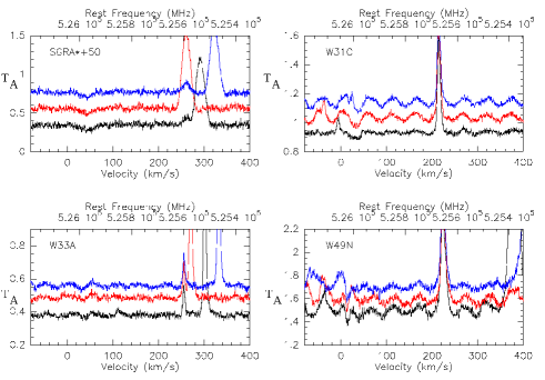
Figure 1: Original $\rm SH^{+}$ spectra (double-sideband antenna temperature $T_{A}$ before removing the standing waves) observed towards SgrA*+50, W31C, W33A, and W49N in the horizontal polarization and for the three different LO settings (in black, red, and blue). For more clarity the red and blue curves have been shifted from the black curve by 0.2 and 0.4 K (for the SgrA*+50 data), and by 0.1 and 0.2 K (for the W31C, W33A, and W49N data).

The observations were carried out from March to October 2010 and in April 2011 towards the eight submillimetre background continuum sources listed in Table 1 (with their Galactic coordinates, their distance from the Sun, and their measured single-sideband continuum temperature $T_{c}$ in K at $\sim 830$ and $\sim 530$ GHz). Using the dual-beam switch (DBS) mode (with a throw at 3’ from the source) and the wide-band spectrometer (WBS) of Herschel/HIFI (see Roelfsema et al. 2012 for a detailed description of the properties and performances of HIFI), we observed

• the $J=1\leftarrow 0$ absorption lines of $\rm CH^{+}$ and $\rm{}^{13}CH^{+}$, in the upper and lower sidebands of band 3a,

• and the $F=3/2\leftarrow 1/2$, $5/2\leftarrow 3/2$, and $3/2\leftarrow 3/2$ hyperfine components of the $N,J=1,2\leftarrow 0,1$ absorption line of $\rm SH^{+}$, in the lower sideband of band 1a.

The data obtained towards SgrB2(N) were part of the full HIFI spectral scan performed by the HEXOS key programme; the corresponding double-sideband spectra were deconvolved into single-sideband spectra, including the continuum (Comito & Schilke 2002). Towards the other sources, the observations were performed in the framework of the PRISMAS key programme; to separate spectral features from upper and lower sidebands of the WBS spectrometer, each transition was observed using three slightly different settings of the local oscillator (LO) frequency, adapted to induce a relative velocity shift of $\sim 30$ km s^-1 between the two sidebands. The spectroscopic parameters of the observed lines are listed in Table 2, along with the rms noise levels relative to the single-sideband continuum intensities obtained with an on-source integration time ranging from 1 to 20 min. In these frequency ranges, the WBS resolution of 1.1 MHz corresponds to velocity resolutions of $\sim 0.36$ km s^-1 for the $\rm CH^{+}$ and $\rm{}^{13}CH^{+}$ transitions, and of $\sim 0.57$ km s^-1 for the $\rm SH^{+}$ transitions, and the Herschel HPBW is 26” at 835 GHz and 41” at 526 GHz.

The data were calibrated with hot and cold blackbodies (Roelfsema et al. 2012), reduced using the standard Herschel pipeline to Level 2, and subsequently analysed using the Herschel Interactive Processing Environment (HIPE v5.1, Ott et al. 2010). The final analysis was performed with the GILDAS-CLASS90 software (Pety 2005), and a set of Fortran95 numerical routines that we developed. While the signals measured in the two orthogonal polarizations that were obtained with the three LO settings agreed excellently for both the $\rm CH^{+}$ and $\rm{}^{13}CH^{+}$ line observations, the $\rm SH^{+}$ spectra, displayed in Fig. 1, exhibit standing waves (SW) of identified origin and removed using the HIPE sine wave fitting task FitHifiFringe (FHF). Since the inferred detected opacities of $\rm SH^{+}$ are low, and since the period and the amplitude of the waves are similar to the size and the depth of the $\rm SH^{+}$ absorption features (see Fig. 1), the resulting spectra were sensitive to the FHF input parameters: several plausible solutions were found depending on the number of sub-bands taken into account for the fit, the number of sine waves to remove, and the use of a frequency mask. We estimated a maximal error of 50 % on the deepest absorption features of G34.3+0.1 and W51, 30 % on those of W33A, and W31C and 10 % on the others. The latter value is comparable to that due to the uncertainties on the beam efficiency and the sideband gain ratio (Roelfsema et al. 2012).

For each transition and both polarizations, we obtained an average spectrum by combining the data from the three observations with different LO settings. Because we are interested in the velocity structure and the properties of the absorbing gas, the spectra in both polarizations were normalized to their respective continuum temperature. As in Falgarone et al. (2010), we used the saturated shape of the $\rm CH^{+}$ absorption line profiles to measure the sideband gain ratios $R$ at 835.1375 GHz, defined as the ratio of the continuum temperatures in the lower and upper sidebands. For all spectra with saturated absorption lines, we found $R\sim 0.9-1$ and $R\sim 0.7-0.8$ in the horizontal and vertical polarizations, respectively. We finally used these values at 835 GHz, and $R=1$ at 830 GHz and 526 GHz, to combine the data from both polarizations, and obtain the final average spectra (with rms noise levels given in Table 2) shown in Fig. 2 as functions of the LSR (local standard of rest) velocity. This figure illustrates the quality of the baselines over the large bandwidth for most of the spectra. The strong emission lines detected in the spectra shown in Figs. 1 and 2 were identified as the $\rm HCO^{+}$ $(6\rightarrow 5)$ and $\rm H_{2}CO$ $(6\rightarrow 5)$ transitions near 535.1 GHz and 525.6 GHz, three methanol lines near 829.9 GHz and 830.3 GHz, and the SO₂ emission band near 835 GHz, emitted by the SFRs themselves.

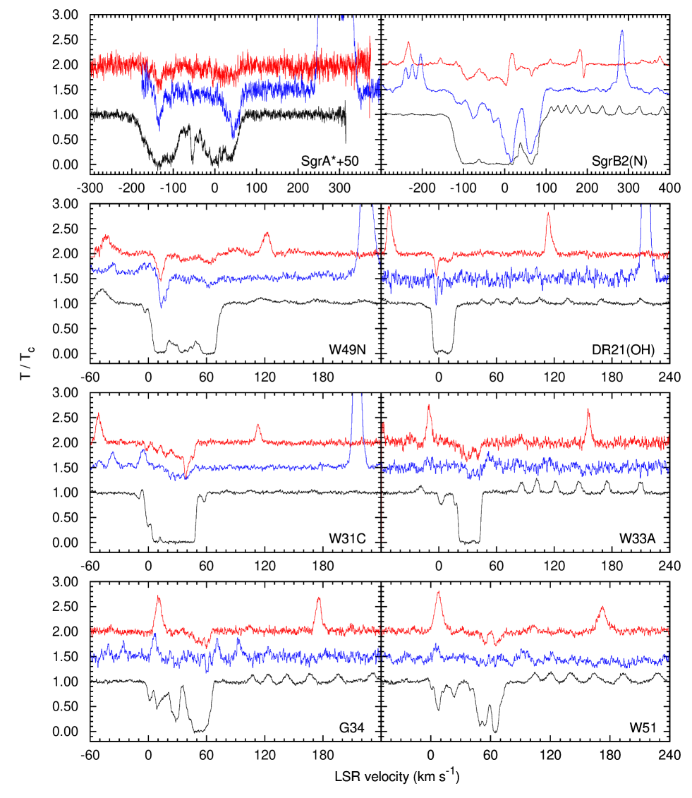
Figure 2: Spectra observed at the frequencies of the ground-state transitions of $\rm CH^{+}$ (black), $\rm{}^{13}CH^{+}$ (red), and $\rm SH^{+}$ (blue) in the direction of DR21(OH), G34.3+0.1, W31C, W33A, W49N, W51, SgrA*+50, and SgrB2(N). All spectra have been normalized to the continuum temperatures. To make the absorption features discernible, the $\rm{}^{13}CH^{+}$ and $\rm SH^{+}$ signals were mutiplied by a factor of 2 towards SgrA*+50, and SgrB2(N), and by factors of 2 and 3, respectively, towards the other sources. For more clarity the $\rm{}^{13}CH^{+}$ and $\rm SH^{+}$ spectra were shifted from the $\rm CH^{+}$ spectra by 0.5 and 1.0.

2.2 Deconvolution of the $\rm SH^{+}$ hyperfine structure

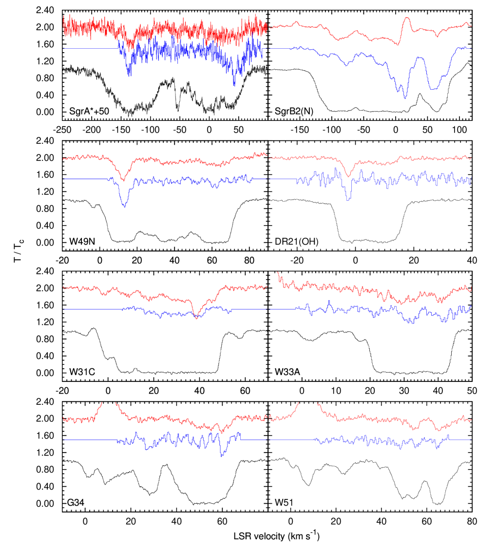
Figure 3: Absorption profiles observed in the direction of DR21(OH), G34.3+0.1, W31C, W33A, W49N, W51, SgrA*+50, and SgrB2(N) in the ground-state transitions of $\rm CH^{+}$ (black) and $\rm{}^{13}CH^{+}$ (red), and in the main hyperfine component (see Tab. 2) of the ground-state transition of $\rm SH^{+}$ (blue). All spectra have been normalized to the continuum temperatures. To make the absorption features discernible, the $\rm{}^{13}CH^{+}$ and $\rm SH^{+}$ signals were mutiplied by a factor of 2 towards SgrA*+50, and SgrB2(N), and by factors of 2 and 3, respectively, towards the other sources. For more clarity the $\rm{}^{13}CH^{+}$ and $\rm SH^{+}$ spectra were shifted from the $\rm CH^{+}$ spectra by 0.5 and 1.0. The x- and y- scales were chosen to display the velocity structure of the absorption features in detail.

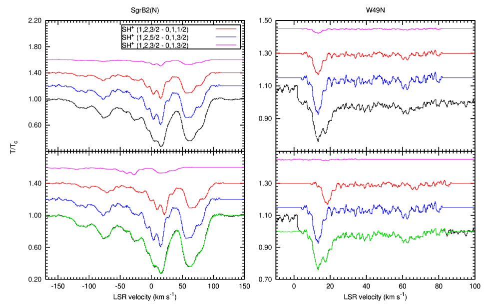
Figure 4: Result of the hyperfine structure deconvolution code applied on the $\rm SH^{+}$ $(1,2\leftarrow 0,1)$ absorption spectrum observed towards SgrB2(N) and W49N. The top panel displays the original data and the resulting decomposition in three hyperfine components, aligned to the same velocity scale. The hyperfine components are shifted by their velocity shift $\Delta\upsilon_{h}$ (see Table 2) in the bottom panels, to show how they can be combined (green line) to reproduce the original data (black line). For more clarity, the hyperfine components were vertically shifted from the original data.

Unfortunately (see Table 2), the velocity shifts $\Delta\upsilon_{h}$ associated with the $\rm SH^{+}$ hyperfine transitions are smaller than the observed velocity ranges of the $\rm SH^{+}$ absorption spectra, and prevent us from performing a direct cross comparison of the velocity profiles of the $\rm SH^{+}$, $\rm CH^{+}$, and $\rm{}^{13}CH^{+}$ lines. To solve this problem, we developed a numerical procedure to extract the signal associated with each hyperfine transition, solving the following set of equations for $\tau_{r}(\upsilon)$, over the entire absorption velocity domain,

$$\sum_{k=1}^{N_{h}}I_{h}(k)\,\tau_{r}(\upsilon-\Delta\upsilon_{h}(k))=-{\rm ln}\left[T(\upsilon)/T_{\rm c}\right],$$ (1)

where $N_{h}$, $I_{h}$, $\tau_{r}$, and $T(\upsilon)/T_{c}$ are the number of hyperfine transitions, the intensities relative to the strongest hyperfine component, the opacity of the reference hyperfine transition, and the normalized line profile (line/continuum), respectively. The resulting spectra are shown in Fig. 3, and, as an example, the outcome of the hyperfine decomposition code, applied to the absorption lines observed towards SgrB2(N) and W49N, is shown in Fig. 4. This figure illustrates the excellent agreement between the original data (in black) and the spectra rebuilt after decomposition (in green).

The $\rm{}^{13}CH^{+}$ $J=1\leftarrow 0$ line also exhibits a spin-rotation splitting (Amano 2010), although the associated $F=3/2\leftarrow 1/2$ and $F=1/2\leftarrow 1/2$ transitions are separated by only 1.636 MHz ($\sim 0.59$ km s^-1) and are therefore too close to be individually resolved given the significant velocity dispersion of the gas. This hyperfine structure induces a systematic broadening of the absorption velocity components that depends on their $FWHM$ $\Delta\upsilon_{\rm real}$ : for $\Delta\upsilon_{\rm real}$ varying between 2 and 10 km s^-1 the broadening ranges between 4% and 0.1%. Since this error is far smaller than that imputable to the rms noise levels of the $\rm{}^{13}CH^{+}$ spectra (see Sect. 3), we chose to ignore the hyperfine structure of $\rm{}^{13}CH^{+}$ in the following analysis.

The spectra shown in Fig. 3 are highly structured and have the following remarkable properties: (1) thanks to the high sensitivity of the HIFI receiver, the $\rm SH^{+}$ ion is seen in absorption along every line of sight; (2) all hydride lines are detected in absorption, and within the limits imposed by the signal/noise (S/N) ratio, $\rm CH^{+}$  $\rm{}^{13}CH^{+}$  and $\rm SH^{+}$ absorptions are detected over the whole velocity range of the foreground matter along each line of sight; (3) although the opacity ratios vary from one line of sight to another and from one velocity range to another, the velocity structure of $\rm SH^{+}$ is similar to those of $\rm CH^{+}$ and $\rm{}^{13}CH^{+}$. It is the similarity and differences of these absorption line profiles that are the focus of the present study.

3 Analysis of the line profiles

3.1 Multi-Gaussian decomposition

As in Godard et al. (2010), the decomposition of the spectra in velocity components was deduced through a multi-Gaussian fitting procedure that we developed, based on the Levenberg-Marquardt algorithm, which takes advantage of the information carried by the hyperfine structure of a given transition. This algorithm is applied to adjust, in the least-squares sense, the minimal number of Gaussians required to describe the data within the observational errors without introducing any systematic effect. The number of Gaussians was increased, for instance, when we visually spotted serpentine curves - characteristic of poor fits in the line wings - in the residuals. Thus, for each transition, the observed normalized line profile (line/continuum) is written

$$\frac{T(\upsilon)}{T_{\rm c}}={\rm exp}\left[-\sum_{j=1}^{N_{c}}\sum_{k=1}^{N_{h}}I_{h}(k)\,\tau_{0}(j)\,e^{-\frac{1}{2}\left[\frac{\upsilon-\upsilon_{0}(j)-\Delta\upsilon_{h}(k)}{\sigma_{0}(j)}\right]^{2}}\right],$$ (2)

where $\tau_{0}$, $\upsilon_{0}$, and $\sigma_{0}$ are the usual Gaussian fit parameters. All spectra were decomposed independently from one another, without imposing any constraints on the Gaussian parameters. The choice of the input parameters, namely the initial values of $\upsilon_{0}(j)$ and $\sigma_{0}(j)$ for each velocity components $j$, was guided by the comparison of the different lines observed towards each source. To correctly determine the opacity of weak absorption features blended with saturated lines, as observed in the $\rm CH^{+}$ spectra, we applied an empirical model constrained by the wings of the saturated line profiles. The results of the multi-Gaussian decomposition procedure and the associated errors on the Gaussian parameters are given in Table LABEL:TabFit of Appendix A, and the resulting fits and models of the saturated line profiles are displayed in Figs. 10 - 17. Because we aim to compare the kinematic signatures of the $\rm CH^{+}$, $\rm{}^{13}CH^{+}$, and $\rm SH^{+}$ spectra, we discuss below the reliability of the extracted Gaussian components in view of the errors on their parameters.

3.2 Validity and self-consistency of the multi-Gaussian decompositions

Since the decomposition algorithm allows the detection of components with very weak central opacities, the numerical procedure may converge upon Gaussian components whose reality is questionable. To keep only the most reliable velocity components for our subsequent analysis of the linewidths, we applied the following detection criterion: any Gaussian component was considered real if its Gaussian parameters simultaneously verify $\Delta\upsilon>3\sigma(\Delta\upsilon)$ and $\tau>2.5\sigma(\tau)$, where $\sigma(\Delta\upsilon)$ and $\sigma(\tau)$ are the errors on $\Delta\upsilon$ and $\tau$ respectively. The resulting confirmed or uncertain Gaussian components (in the following C-components and U-components) are indicated in Table LABEL:TabFit (in columns 4, 8, and 12), and in Figs. 10 - 17 (solid red and dashed blue curves) of Appendix A.

In total we found that 25 C-components are simultaneously observed in at least two molecular spectra towards DR21(OH), G34.3+0.1, W31C, W33A, W49N, and W51. When compared, the positions of these components are found to agree with one another within their respective error for 18 of them, within 0.5 km s^-1 for 6 of them, and within 1.3 km s^-1 for 1 of them; similarly, out of the 17 common C-components observed towards SgrA*+50 and SgrB2(N), 10 are found to agree with one another within 1 km s^-1, 6 within 2 km s^-1, and 1 within 3.5 km s^-1. Except for the $\rm SH^{+}$ components at -126 km s^-1 observed towards SgrA*+50 these shifts in the central positions are at least four times smaller than the corresponding Gaussian linewidths. Moreover, many of the U-components have corresponding C-components in other species, indicating that the fitting process is robust and that the selection method is severe.

These concordances combined with the strict selection on the Gaussian parameters suggest that all C-components are real detections and not artefacts caused by noise or the standing waves removing procedure.

3.3 Comparison of the Gaussian linewidths

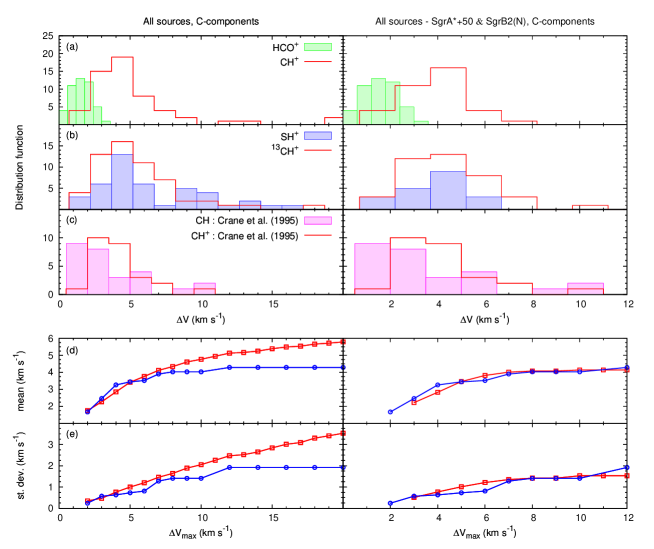
Figure 5: Top: (a) and (b) histogram of the linewidths of the $\rm CH^{+}$, $\rm{}^{13}CH^{+}$, $\rm SH^{+}$ (this work), and $\rm HCO^{+}$ (Godard et al. 2010) velocity components obtained with the multi-Gaussian decomposition procedure (see Table LABEL:TabFit); (c) linewidth distributions of $\rm CH^{+}$ and CH observed by Crane et al. (1995) in the local diffuse medium. Bottom: first- (mean) and second- (standard deviation) order moments of the $\Delta\upsilon$ distributions issued from the combined $\rm CH^{+}$, $\rm{}^{13}CH^{+}$, and $\rm SH^{+}$ data (red squares) and from the $\rm CH^{+}$ data observed in the solar neighbourhood (blue circles); the moments are computed over increasing $\Delta\upsilon$ intervals: mean = $\int_{0}^{\Delta\upsilon_{\rm max}}\Delta\upsilon N(\Delta\upsilon)d(\Delta\upsilon)/\int_{0}^{\Delta\upsilon_{\rm max}}N(\Delta\upsilon)d(\Delta\upsilon)$; standard deviation = $[\int_{0}^{\Delta\upsilon_{\rm max}}(\Delta\upsilon-{\rm mean})^{2}N(\Delta\upsilon)d(\Delta\upsilon)/\int_{0}^{\Delta\upsilon_{\rm max}}N(\Delta\upsilon)d(\Delta\upsilon)]^{1/2}$, where $N(\Delta\upsilon)$ is the linewidth distribution.

In Fig. 5, we display the distributions of linewidths associated with the C-components extracted from the $\rm CH^{+}$, $\rm{}^{13}CH^{+}$, and $\rm SH^{+}$ spectra. To emphasize the differences observed along the Galactic centre sight lines ($l\sim 0$), these distributions are computed for all sight lines (left panels), and for the $l\neq 0$ sight lines only (right panels). As a comparison, the linewidth distributions of the $\rm HCO^{+}$ ground state radio transition observed by Godard et al. (2010) towards W31C, W49N, W51, and G34.6 are displayed in panels (a), and those of CH and $\rm CH^{+}$ visible transitions observed at high spectral resolution ($\sim 0.3$ km s^-1) in the local diffuse medium by Crane et al. (1995) are shown in panels (c) of Fig. 5. Lastly, panels (d) and (e) of Fig. 5 display the first- and second-order moments of the $\Delta\upsilon$-distributions issued from the combined $\rm CH^{+}$, $\rm{}^{13}CH^{+}$, and $\rm SH^{+}$ data (red squares) and from the $\rm CH^{+}$ data observed in the solar neighbourhood (blue circles). In panels (a), the histogram of $\rm HCO^{+}$ linewidths is narrower and peaks at lower values than those of the submillimetre lines of $\rm CH^{+}$, $\rm{}^{13}CH^{+}$, and $\rm SH^{+}$. Conversely, the histogram of the visible $\rm CH^{+}$ data, characterising the local diffuse interstellar matter, is very similar to that of the submillimetre data. We discuss the validity and the significance of these comparisons below.

To demonstrate that the absence of narrow velocity components in the $\rm CH^{+}$, $\rm{}^{13}CH^{+}$, and $\rm SH^{+}$spectra is real and not due to a limitation of our extraction algorithm, we have derived the minimum width of a Gaussian component of optical depth $\tau_{0}$ that can be extracted from a given profile characterised by a noise $\sigma_{\tau}$ at the velocity resolution $\delta\upsilon$. Because $\sigma_{\tau}$ scales inversely with the square root of the velocity resolution, a component detected at a $3\sigma_{\tau}$ level necessarily verifies

$$\Delta\upsilon\geqslant\delta\upsilon\left[3\sigma_{\tau}/\tau_{0}\right]^{2}.$$ (3)

While the noise level of the $\rm SH^{+}$ spectra towards SgrA*+50, DR21(OH), G34.3+0.1, and W33A forbids us to extract components with linewidth smaller than 1 km s^-1, that of all the other spectra is small enough to allow us to detect narrow velocity structures down to two velocity channels (0.72 km s^-1 for $\rm CH^{+}$ and $\rm{}^{13}CH^{+}$, and 1.14 km s^-1 for $\rm SH^{+}$). Therefore the scarcity of components in the first bin [0 ; 2 km s^-1] of the $\rm CH^{+}$, $\rm{}^{13}CH^{+}$, and $\rm SH^{+}$ histograms is not a noise artefact.

Now, can we compare these linewidth distributions with one another? Because the S/N ratios of $\rm HCO^{+}$ (see Table. 1 of Godard et al. 2010) and $\rm CH^{+}$ (see Table. 2) profiles are high and comparable, those two sets of spectra are decomposed with the same level of detection. The noise therefore affects the statistics of the component linewidths at the same level. The same is true for the lines of $\rm SH^{+}$ and $\rm{}^{13}CH^{+}$, which have comparable, though poorer, S/N ratios. Finally, because $\rm CH^{+}$ and $\rm{}^{13}CH^{+}$ necessarily bear the same dynamical signatures, all distributions displayed in Fig. 5 can be compared with one another.

We recall that all absorption spectra have been decomposed into Gaussians independently from one another, without imposing the same velocity centroids or width to the different velocity components of a given line of sight. In addition, since the most intense $\rm SH^{+}$ components are saturated in $\rm CH^{+}$, and because the moderate S/N ratio of the $\rm{}^{13}CH^{+}$ and $\rm SH^{+}$ data prevents us from observing the low-opacity structures detected in the $\rm CH^{+}$ spectra, the respective distributions do not correspond to the same velocity components. It is therefore remarkable that the distributions of the $\rm CH^{+}$, $\rm{}^{13}CH^{+}$, and $\rm SH^{+}$ widths of the Gaussian velocity components are so similar, even identical within the statistical uncertainty. They exhibit a common pattern: a peak (hereafter called P1), observed towards all the sources, defined by a first- (mean) and a second- (standard deviation) order moments of $4.2\pm 0.2$ km s^-1 and $1.5\pm 0.1$ km s^-1, respectively, and an extended tail (hereafter called P2), observed only on the Galactic centre sight lines (left panels), with $\Delta\upsilon$-values up to 20 km s^-1.

Because the lines of sight sample kiloparsecs of interstellar material in the Galaxy, the patterns P1 and P2 result from the small-scale dynamics of the production processes of $\rm CH^{+}$ and $\rm SH^{+}$, the turbulent dynamics of the diffuse ISM, and the Galactic dynamics. The comparison between the left and right (d) and (e) panels of Fig. 5 shows that the first- and second-order moments of the $\Delta\upsilon$ distributions are the same for the components of the Galactic ISM along the $l\neq 0$ sight lines and the visible $\rm CH^{+}$ lines sampling the solar neighbourhood (defined by first- and second-order moments of $4.3\pm 0.4$ km s^-1 and $1.85\pm 0.3$ km s^-1, respectively). Because the latter is unaffected by the Galactic dynamics, this similarity suggests that the peak P1 results from the dynamics of the formation processes of $\rm CH^{+}$ and $\rm SH^{+}$ convolved with that of the turbulence of the diffuse gas. Because the tail of the $\Delta\upsilon$ distributions is observed only on the Galactic centre sight lines, and because the high absorption dips ($\Delta\upsilon>8$ km s^-1) observed on the $l\neq 0$ sight lines can be decomposed into many narrow components (as performed by Godard et al. 2010 with the $\rm HCO^{+}$ spectra), we conclude that P2 is caused by the Galactic dynamics only.

Lastly we note that while the first- and second-order moments of peak P1 both agree with those of the $\Delta\upsilon$ distribution obtained by Crane et al. (1995) within the statistical uncertainties, they also substantially differ from those of the $\rm CH^{+}$ $\Delta\upsilon$ distribution derived in the solar neighbourhood by Pan et al. (2004), who find first- and second-order moments of $3.3\pm 0.04$ km s^-1 and $0.4\pm 0.03$ km s^-1. As proposed by Pan et al. (2005), these differences may originate from their profile fitting method: (1) the number of $\rm CH^{+}$ components and their position were constrained by the observations of other species, possibly unrelated chemically (e.g. CN, CO, Ca), and (2) a maximal value of $\Delta\upsilon$ of 5.8 km s^-1 was set.

4 Analysis of the integrated opacities

Since the multi-Gaussian decomposition of $\rm CH^{+}$, $\rm{}^{13}CH^{+}$, and $\rm SH^{+}$ absorption profiles provides sets of C-components that do not always strictly coincide in velocity and width, and sets of U-components that sometimes clearly correspond to real absorption but with width and depth poorly constrained, our subsequent analysis and comparison of the column densities and abundances of these species is based on integrals of opacities computed over broad velocity intervals corresponding to marked absorption features common to all lines. These broad intervals (typically 5 to 20 km s^-1) are given in the two first columns of Table LABEL:TabIntTau. The column densities given in columns 4, 5, and 6 of Table LABEL:TabIntTau are derived assuming a single excitation temperature of 4.4 K for $\rm{}^{12}CH^{+}$ and $\rm{}^{13}CH^{+}$, and of 3.0 K for $\rm SH^{+}$ (see Appendix B). Following the method set in Sect. 3.2 to keep only the most reliable absorption features, a $3\sigma$ detection level was adopted. Throughout, every measurement below this level is considered as a lower limit. Conversely, we adopt a conservative lower limit of 2.3 on the optical depth for the saturated velocity intervals (Neufeld et al. 2010b).

4.1 Variation of the ¹²C/¹³C isotopic ratio across the Galactic disk

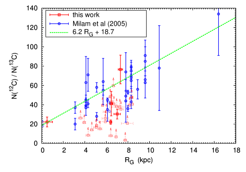
Figure 6: $N({\rm{}^{12}C})/N({\rm{}^{13}C})$ column density ratio as a function of the galactocentric distance $R_{G}$. The red squares are from this work, and therefore evaluated with measurements of the $N({\rm{}^{12}CH^{+}})/N({\rm{}^{13}CH^{+}})$ column density ratio. The blue circles are from previous measurements of the $N({\rm{}^{12}CN})/N({\rm{}^{13}CN})$, $N({\rm{}^{12}CO})/N({\rm{}^{13}CO})$, and $N({\rm H_{2}^{12}CO})/N({\rm H_{2}^{13}CO})$ column density ratios (Milam et al. 2005 and references therein) while the green curve corresponds to a linear least-squares fit applied to these data.

In Fig. 6, we display the ${\rm{}^{12}C}/{\rm{}^{13}C}$ column density ratio derived from the present $\rm{}^{12}CH^{+}$ and $\rm{}^{13}CH^{+}$ data as a function of the Galactocentric distance $R_{G}$ (given in columns 7 and 8 of Table LABEL:TabIntTau) which was computed assuming a flat Galactic rotation curve. We compared these results to those deduced from previous observations of CN, CO, $\rm H_{2}CO$ and their respective isotopologues (Milam et al. 2005). We found that the five firm values (indicated in Table 3) derived from the simultaneous detections of ${\rm{}^{12}CH^{+}}$ and ${\rm{}^{13}CH^{+}}$ absorption lines over the same velocity range are consistent with those derived from the neutral species. The 25 lower limits inferred from saturated $\rm{}^{12}CH^{+}$ lines (dashed symbols) are also consistent with Milam et al. (2005). This result not only suggests that the isotopic ratios measured with ions and neutrals are not substantially influenced by chemical fractionation processes, but it also validates the use of the empirical relation

$${\rm{}^{12}C}/{\rm{}^{13}C}=6.2(\pm 1.0)R_{G}+18.7(\pm 7.4)$$ (4)

found by Milam et al. (2005) to infer the $\rm{}^{12}CH^{+}$ column densities from those measured in the $\rm{}^{13}CH^{+}$ spectra. The ${\rm{}^{12}C}/{\rm{}^{13}C}$ ratio and $N({\rm{}^{12}CH^{+}})$ computed from Eq. 4 for the velocity intervals towards DR21(OH), G34.3+0.1, W31C, W33A, W49N, and W51 are given in columns 9 and 10 of Table LABEL:TabIntTau. Towards SgrA*+50 and SgrB2(N), because most of the gas appears to be associated with the Galactic centre environment (Rodriguez-Fernandez et al. 2006), a ${\rm{}^{13}C}/{\rm{}^{12}C}$ abundance ratio of 20 is assumed everywhere except for the velocity interval -20 to +30 km s^-1, a velocity domain where the absorption features are also associated with gas in the Galactic plane, and where we use two alternative values, 20 and 60, to bracket the result.

The uncertainties given in Eq. 4 correspond to the standard deviation of the best least-squares fit performed by Milam et al. (2005) on the CN, CO, and $\rm H_{2}CO$ data. They do not take into account the uncertainty on $R_{G}$ due to the random motion of interstellar clouds. To do so, we relied on the analysis of the HI emission in the first Galactic quadrant by Elmegreen & Elmegreen (1987): they found that a large part of the mass of the diffuse gas is distributed into $\sim$ 200 pc superclouds, separated along spiral arms by 1.5 kpc. Their one-dimensional internal velocity dispersion of 5.3 km s^-1 is the main source of uncertainty on $R_{G}$. Taking into account the $(l,v)$ location of the absorbing gas observed towards each source (see the equation of $R_{G}$ in the caption of Table LABEL:TabIntTau), we obtain a maximal uncertainty of about 30 % on $R_{G}$. When combined with the errors given in Eq. 4, we find a total uncertainty of about 50% on the ${\rm{}^{12}C}/{\rm{}^{13}C}$ ratio and the subsequent $N({\rm{}^{12}CH^{+}})$ given in columns 9 and 10 of Table LABEL:TabIntTau.

4.2 Comparison of the column densities of $\rm CH^{+}$ and $\rm SH^{+}$ 

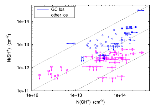
Figure 7: $\rm SH^{+}$ column density as a function of the $\rm CH^{+}$ column density per broad velocity interval (see Table LABEL:TabIntTau). The open squares and open circles are from the present analysis and from Menten et al. (2011), respectively. The blue and purple points are from the absorption lines observed along the Galactic centre sight lines (SgrA*+50, SgrB2(N), and SgrB2(M)) and along the other sight lines (DR21(OH), G34.3+0.1, W31C, W33A, W49N, and W51), respectively. The black dashed, dotted, and dashed-dotted curves indicate $N({\rm SH^{+}})/N({\rm CH^{+}})$ ratios of 0.01, 0.1, and 1, respectively.

Fig. 7 displays the $\rm SH^{+}$ and $\rm CH^{+}$ column densities inferred for each broad velocity interval. The $\rm CH^{+}$ column densities were derived either from the $\rm{}^{12}CH^{+}$ profile, where unsaturated, or from $\rm{}^{13}CH^{+}$ and the above isotopic ratio in the other case. The data set includes the results of the present study and those obtained by Menten et al. (2011) towards SgrB2(M). While Menten et al. (2011) reported the detection of two absorption components at $N({\rm CH^{+}})\sim 3\times 10^{12}$ and $N({\rm SH^{+}})\sim 10^{13}$ $\,{\rm cm}^{-2}$, we removed those points from Fig. 7 because the $\rm{}^{13}CH^{+}$ spectrum in the corresponding velocity range clearly exhibits contamination of the absorption features by a strong and broad emission line. Last, we note that the few points at $N({\rm CH^{+}})<10^{13}$ $\,{\rm cm}^{-2}$ correspond to the faintest $\rm{}^{12}CH^{+}$ absorption features. Since they are not detected in $\rm SH^{+}$, these points weakly constrain our subsequent analysis of the $\rm SH^{+}$/$\rm CH^{+}$ratio.

Taking into account the upper and lower limits shown in Fig. 7, we find that $N({\rm CH^{+}})$ and $N({\rm SH^{+}})$ span more than two orders of magnitude and that the ${\rm SH^{+}}/{\rm CH^{+}}$ column density ratio varies from less than 0.01 to 1. Interestingly, the $N({\rm SH^{+}})/N({\rm CH^{+}})$ ratios observed towards SgrB2(M), SgrB2(N), and SgrA*+50 are very similar, with a mean value of $0.28\pm 0.02$, $\sim$ 9 times higher than that towards DR21(OH), G34.3+0.1, W31C, W33A, W49N, and W51, $\left<N({\rm SH^{+}})/N({\rm CH^{+}})\right>\sim 0.03\pm 0.007$. The above difference in the mean ${\rm SH^{+}}/{\rm CH^{+}}$ ratio is much larger than the 50 % uncertainty on the computed ${\rm{}^{12}C}/{\rm{}^{13}C}$ ratio. Moreover, we obtain the same difference of values if we use only the few points detected in $\rm{}^{12}CH^{+}$. It is therefore unlikely that this difference can be ascribed to an uncertainty on the ${\rm{}^{12}CH^{+}}/{\rm{}^{13}CH^{+}}$ ratio. Last, Daflon & Cunha (2004) found that carbon and sulfur have similar abundance gradients across the Galactic disk (with slopes of -0.037 and -0.040 dex kpc^-1, respectively). Consequently, the difference observed in the ${\rm SH^{+}}/{\rm CH^{+}}$ column density ratios measured on the $l\sim 0$ and $l\neq 0$ sight lines is most likely tracing variations of both the physical and chemical conditions of the diffuse gas sampled in each case.

Finally, with a correlation coefficient of 0.1, no evident chemical relationship seems to stand out from Fig. 7, a surprising finding in view of the fact that $\rm CH^{+}$ and $\rm SH^{+}$ are clearly linked by their dynamics (see Sect. 3.3). However, this lack of correlation applies to the column densities. In the following, we discuss the properties of the abundances relative to hydrogen, a discussion that requires the knowledge of $N_{\rm H}$.

4.3 Estimation of the hydrogen column densities in the broad velocity intervals

To (1) estimate the mean molecular abundances that are to be compared with the chemical model predictions (Godard et al., in preparation), and (2) to establish a possible relation between the $\rm CH^{+}$ and $\rm SH^{+}$ abundances, it is essential to estimate the hydrogen column density ${N_{\rm H}}$ in the broad velocity intervals over which $N({\rm CH^{+}})$ and $N({\rm SH^{+}})$ are measured. Since the molecular fraction of the gas where $\rm CH^{+}$ and $\rm SH^{+}$ are detected is low (0.4 on average, see Appendix C), both atomic and molecular hydrogen HI and $\rm H_{2}$ are needed to estimate ${N_{\rm H}}$.

The method consists in separately evaluating the column densities of HI and $\rm H_{2}$, using the VLA observations of the $\lambda 21$ cm absorption line of H (Koo 1997; Fish et al. 2003; Dwarakanath et al. 2004; Pandian et al. 2008; Lang et al. 2010) and a relevant tracer for the molecular hydrogen because $\rm H_{2}$ is not directly observable. Then, ${N_{\rm H}}=N(HI)+2N({\rm H_{2}})$. In Appendix C we discuss the validity of using the HIFI observations of CH and HF to compute the $\rm H_{2}$ column densities. If available, HF is preferentially used in the following section to infer $N({\rm H_{2}})$ and the ensuing $\rm CH^{+}$, $\rm{}^{13}CH^{+}$, and $\rm SH^{+}$ mean abundances. If not, $N({\rm H_{2}})$ is derived from CH, assuming a HF/CH mean abundance ratio of 0.4 (a value defined with a large standard deviation of 0.25), deduced from columns 5 and 6 of Table LABEL:TabHI. Last, we compare these values of ${N_{\rm H}}$ to those inferred, as in Godard et al. (2010), from the analysis of the 2MASS survey (Cutri et al. 2003). Marshall et al. (2006) have measured the near infrared colour excess in large areas of the inner Galaxy ($|l|<100^{\circ}$, $|b|<10^{\circ}$) to obtain the visible extinctions ($A_{V}\sim 10A_{K}$), providing an estimate of the total hydrogen column density along the lines of sight. However, because of the low resolution of the 2MASS extinction analysis ($\sim 15$ arcmin), the uncertainty on ${N_{\rm H}}$ (computed as the standard deviation of the extinction measured along the four closest lines of sight surrounding a given source) can be important, and is as high as 50% for DR21(OH), W31C, and W33A. The last columns of Table LABEL:TabHI show that these two independent measurements of ${N_{\rm H}}$ differ by less than 25 %.

5 Results and discussion

5.1 Chemical properties of the gas seen in absorption

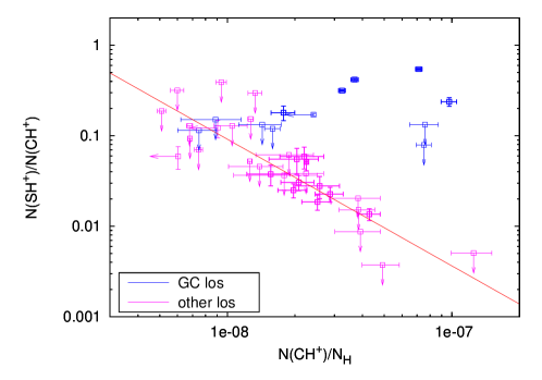
Figure 8: $N({\rm SH^{+}})/N({\rm CH^{+}})$ column density ratio as a function of the $\rm CH^{+}$ mean abundance. The $\rm CH^{+}$, $\rm SH^{+}$, and H column densities are computed from $\rm CH^{+}$, $\rm{}^{13}CH^{+}$, $\rm SH^{+}$, HI, HF, and CH opacities integrated over the velocity intervals given in Tables LABEL:TabIntTau and LABEL:TabHI. The blue and purple points are from the absorption lines observed along the Galactic centre sight lines (SgrA*+50 and SgrB2(N)) and along the other sight lines (DR21(OH), G34.3+0.1, W31C, W33A, W49N, and W51), respectively. The red line corresponds to a least-squares fit of the latter data.

In Fig. 8, we display the $N({\rm SH^{+}})/N({\rm CH^{+}})$ column density ratio as a function of the $\rm CH^{+}$ mean abundance (with respect to the total hydrogen column density $N_{\rm H}$) integrated over the velocity intervals given in Table LABEL:TabHI. Because Menten et al. (2011) used a different method than we did to estimate the $\rm H_{2}$ column densities the data obtained towards SgrB2(M) are not included in this plot. We found that both the mean abundances and the abundance ratios vary by two orders of magnitude in the diffuse ISM sampled by those lines of sight. In addition, Fig. 8 reveals major differences between the results obtained on the $l\sim 0$ and the $l\neq 0$ sight lines. While the $\rm CH^{+}$ mean abundances span the same range of values in both cases, the ${\rm SH^{+}}/{\rm CH^{+}}$ ratio measured towards SgrA*+50 and SgrB2(N) shows no correlation with $N({\rm CH^{+}})/N_{\rm H}$. Conversely, the points corresponding to the observations performed on the $l\neq 0$ sight lines exhibit a trend

$$N({\rm SH^{+}})/N({\rm CH^{+}})\sim 0.09\,\,\big{[}10^{8}\times N({\rm CH^{+}})/N_{\rm H}\big{]}^{-1.4},$$ (5)

with a correlation coefficient of 0.8. These are the results that have to be compared with the predictions of chemical models applied to the diffuse ISM.

5.2 Carbon and sulfur chemistries in the diffuse ISM

5.2.1 UV-driven chemistry

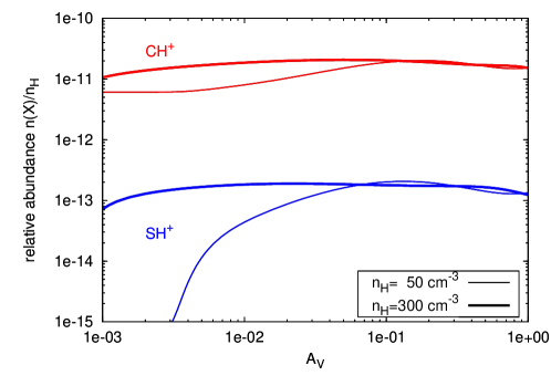
Figure 9: Predictions of two PDR models for gas densities ${n_{\rm H}}=50$ and $300$ $\,{\rm cm}^{-3}$. The $\rm CH^{+}$ (in red) and $\rm SH^{+}$ (in blue) relative abundances are displayed as functions of the shielding $A_{V}$ from the interstellar radiation field for a slab of gas illuminated on one side only.

In a chemistry entirely driven by the UV-radiation field and the cosmic ray particles, the hydrogenation chains of carbon and sulfur, and the subsequent productions of $\rm CH^{+}$ and $\rm SH^{+}$  are initiated by the radiative associations of $\rm C^{+}$ and $\rm S^{+}$ with molecular hydrogen,

$$\begin{array}[]{l l l l l l l}{\rm C}^{+}&+&{\rm H}_{2}&\rightarrow&{\rm CH}_{2}^{+}&+&\gamma\,\,{\rm and}\\[6.0pt] {\rm S}^{+}&+&{\rm H}_{2}&\rightarrow&{\rm SH}_{2}^{+}&+&\gamma,\\ \end{array}$$ (6)

two reactions with long timescales: $2\times 10^{6}\,{\rm yr}\,\,f_{{\rm H}_{2}}^{-1}\left(50\,{\,{\rm cm}^{-3}}/{n_{\rm H}}\right)$ and $1\times 10^{8}\,{\rm yr}\,\,f_{{\rm H}_{2}}^{-1}\left(50\,{\,{\rm cm}^{-3}}/{n_{\rm H}}\right)$, respectively (Herbst 1985; Herbst et al. 1989), where $f_{{\rm H_{2}}}$ is the molecular fraction defined as $f_{{\rm H_{2}}}=2n({\rm H_{2}})/{n_{\rm H}}$. In comparison, $\rm CH^{+}$ and $\rm SH^{+}$ are mainly destroyed by hydrogenation and dissociative recombination,

$$\begin{array}[]{l l l l l l l}{\rm CH}^{+}&+&{\rm H}_{2}&\rightarrow&{\rm CH}_{2}^{+}&+&{\rm H}\,\,{\rm and}\\[6.0pt] {\rm SH}^{+}&+&e^{-}&\rightarrow&{\rm S}&+&{\rm H},\\ \end{array}$$ (7)

two processes with short timescales: $1\,{\rm yr}\,\,f_{{\rm H}_{2}}^{-1}\left(50\,{\,{\rm cm}^{-3}}/{n_{\rm H}}\right)$ and $5\,{\rm yr}\,\,(T/100\,{\rm K})^{0.72}(1.38\times 10^{-4}/x_{e^{-}})(50\,{\,{\rm cm}^{-3}}/{n_{\rm H}})$, respectively. Because of the lack of efficient production pathways to balance their rapid destruction, the $\rm CH^{+}$ and $\rm SH^{+}$ abundances predicted by UV-dominated chemistry are very low. Fig. 9 displays the $\rm CH^{+}$ and $\rm SH^{+}$ relative abundances computed with two models of PhotoDissociation Regions (PDR) illuminated on one side as functions of the shielding from the ISRF $A_{V}$. For the physical conditions of the diffuse gas, we obtain $N({\rm CH^{+}})/N_{\rm H}\sim 1.8\times 10^{-11}$ and $N({\rm SH^{+}})/N_{\rm H}\sim 1.6\times 10^{-13}$, two to four orders of magnitude lower than the observed values, and with a corresponding abundance ratio never higher than 0.01.

5.2.2 Alternative models

In the diffuse interstellar medium sampled by the $l\neq 0$ sight lines, the only production pathways efficient enough to balance the fast destruction of $\rm CH^{+}$ and $\rm SH^{+}$ are

$${\rm C}^{+}+{\rm H}_{2}\rightarrow{\rm CH}^{+}+{\rm H}\quad\Delta E/k=4640{\rm K},\quad{\rm and}$$ (8)

$${\rm S}^{+}+{\rm H}_{2}\rightarrow{\rm SH}^{+}+{\rm H}\quad\Delta E/k=9860{\rm K}.$$ (9)

Since these reactions are highly endothermic, it has been proposed that high $\rm CH^{+}$ and $\rm SH^{+}$ abundances are the signatures of shock waves propagating through the ISM (Draine 1986; Millar et al. 1986). Comparing the predictions of HD and MHD shocks with the $\rm CH^{+}$ column density observed towards $\zeta$ Oph, Draine (1986) and Pineau des Forêts et al. (1986) favoured the MHD case in which $\rm CH^{+}$ and $\rm SH^{+}$ form mainly through ion-neutral friction. Including the sulfur chemistry Millar et al. (1986) and Pineau des Forêts et al. (1986) predicted a ${\rm SH^{+}}/{\rm CH^{+}}$ abundance ratio increasing from 0.01 to 0.4 for a shock speed increasing from 9 to 16 km s^-1, a transverse magnetic field of $5\mu$G and a preshock density of 20 $\,{\rm cm}^{-3}$. These results agree excellently with our observations.

Another scenario, alternative to the shock waves, is the TDR (turbulent dissipation regions) model. In this model the turbulent energy is dissipated in many small-scale magnetized vortices in which the ionized and neutral fluids decouple. Dissipation is caused by both ion-neutral friction and viscous dissipation at the edge of the vortices. Comparing the predictions of TDRs to observations of CH, $\rm CH^{+}$, OH, and $\rm HCO^{+}$ in the local diffuse gas, Godard et al. (2009) also favoured models in which the dissipation is dominated by the ion-neutral friction and where the production of $\rm CH^{+}$ and $\rm SH^{+}$ via reactions 8 and 9 is triggered by the ambipolar diffusion. An analysis of the ${\rm SH^{+}}/{\rm CH^{+}}$ ratio obtained in the framework of the TDR model will be presented in a forthcoming paper (Godard et al. in prep.).

While the scenarios of shocks and vortices could equally apply to gas sampled by the $l\sim 0$ sight lines, an alternative chemical process may be at work there. Large amounts of the diffuse gas detected along SgrA*+50, SgrB2(N), and SgrB2(M) belong to the Central Molecular Zone (CMZ). Because the CMZ is pervaded by a strong X-ray radiation field, high $\rm CH^{+}$ and $\rm SH^{+}$ abundances could be due to regions where $\rm C^{++}$ and $\rm S^{++}$ ions co-exist with $\rm H_{2}$ and form $\rm CH^{+}$ and $\rm SH^{+}$ by the reactions

$${\rm C}^{++}+{\rm H}_{2}\rightarrow{\rm CH}^{+}+{\rm H}^{+},\quad{\rm and}$$ (10)

$${\rm S}^{++}+{\rm H}_{2}\rightarrow{\rm SH}^{+}+{\rm H}^{+},$$ (11)

as proposed by Langer (1978). Using the high rate of reaction (11) obtained by Chen et al. (2003), Abel et al. (2008) found that the predicted $\rm SH^{+}$ column density for molecular gas surrounding an active galactic nucleus is two orders of magnitude higher than that predicted by UV-dominated chemistry. Since rate measurements of reaction (10) point to lower values, this chemical process could account for the high mean ${\rm SH^{+}}/{\rm CH^{+}}$ abundance ratio derived towards SgrA*+50, SgrB2(N), and SgrB2(M) (about nine times higher than that obtained along the other Galactic sight lines, see Sect. 4.2).

The above results are in line with the detection of large amounts of warm diffuse gas recently identified with the 3$\mu m$ absorption lines of $\rm H_{3}^{+}$ (Oka et al. 2005; Geballe & Oka 2010) in the CMZ. The temperature ($\sim 200-300$ K) of the low-density gas phase is found to be considerably higher than that of typical diffuse clouds, and unique to the Galactic CMZ (Goto et al. 2008). They also corroborate the specific dynamics of molecular clouds associated with the Galactic centre regions (e.g. Rodriguez-Fernandez et al. 2006).

6 Summary and perspectives

We have presented the analysis of Herschel/HIFI observations of the ground-state transitions of $\rm CH^{+}$, $\rm{}^{13}CH^{+}$, and $\rm SH^{+}$, all detected in absorption against the submillimetre dust continuum of distant star-forming regions and the Galactic centre sources, SgrA*+50 and SgrB2(N). The velocity range over which the absorption features are detected corresponds to diffuse or transluscent environments. The deconvolution of the hyperfine structure embedded in the $\rm SH^{+}$ $1,2-0,1$ spectra, and the independent decomposition of the absorption domains in Gaussian velocity components allowed us to identify many velocity components per sight line and to perform a cross comparison of the dynamical and chemical signatures of those three species.

This study provides the following main results. (1) The linewidth distributions of $\rm CH^{+}$, $\rm{}^{13}CH^{+}$, and $\rm SH^{+}$ are found to be similar and likely trace the kinematics of the chemical production processes of these species convolved with that of the turbulent and Galactic dynamics of the diffuse ISM. (2) These lines are broad ($\sim 4.2$ km s^-1), similar to those found in visible absorption lines in the solar neighbourhood, and broader than those of $\rm HCO^{+}$ and CN along the same lines of sight. (3) The ${\rm SH^{+}}/{\rm CH^{+}}$ abundance ratio covers a broad range of values from 0.01 to more than 1, shows higher values in warmer environments (such as the Galactic centre clouds), and appears to be proportional to $(N({\rm CH^{+}})/N_{\rm H})^{-1.4}$ in the diffuse gas sampled by the $l\neq 0$ sight lines. (4) As for $\rm CH^{+}$, the $\rm SH^{+}$ abundances cannot be reproduced by UV-driven chemistry in the diffuse gas.

The unique properties of the carbon and sulfur chemistries support the framework of a warm chemistry triggered by turbulent dissipation (either in shocks or intense velocity shears) that selectively enhances the production of $\rm SH^{+}$ for which the formation endothermicity is the highest. A detailed comparison of the TDR model predictions with these observational results will be given in a forthcoming paper (Godard et al. in prep.).

Table 3: Comparison between the column densities of $\rm CH^{+}$, $\rm{}^{13}CH^{+}$, and $\rm SH^{+}$obtained with the integrations of the respective opacities over several velocity intervals. The two last columns contain the ratios $r_{12}=N({\rm SH^{+}})/N({\rm CH^{+}})$ and $r_{13}=N({\rm SH^{+}})/N({\rm{}^{13}CH^{+}})\times{\rm{}^{13}C}/{\rm{}^{12}C}$. In column 10, $\rm CH^{+}$ column densities are inferred from those of $\rm{}^{13}CH^{+}$ and the $\rm{}^{12}C$/$\rm{}^{13}C$ Galactic gradient derived by Milam et al. (2005): $N({\rm CH^{+}})=N({\rm{}^{13}CH^{+}})\times{\rm{}^{12}C}/{\rm{}^{13}C}$. The blank spaces correspond to unusable $\rm{}^{13}CH^{+}$ or $\rm SH^{+}$ data owing to the contamination of an emission line from the SFRs, or because the spectrum measured over the associated velocity interval could not be deconvolved from the $\rm SH^{+}$ hyperfine structure.

$\upsilon_{\rm min}$	$\upsilon_{\rm max}$	$*$	$N$(CH+)b				$N$(SH+)				$N$(13CH+)				$R_{g,{\rm min}}^{a}$	$R_{g,{\rm max}}^{a}$	${\rm{}^{12}C}/{\rm{}^{13}C}$	$N$(CH+)b				$r_{12}$b				$r_{13}$b
(km s-1)	(km s-1)		($10^{13}$ cm-2)				($10^{12}$ cm-2)				($10^{12}$ cm-2)				(kpc)	(kpc)		($10^{13}$ cm-2)				$\times 10$				$\times 10$
SgrA*+50
-215	-198			0.	3	$\pm$ 0.1					$<$	0.	6				20	$<$	1.	2
-198	-168			3.	4	$\pm$ 0.1					$<$	0.	8				20	$<$	1.	6
-168	-150		$>$	6.	9		$<$	3.	4			2.	3	$\pm$ 0.6			20		4.	7	$\pm$ 1.3	$<$	0.	5		$<$	0.	7
-150	-123		$>$	19.	1			56.	8	$\pm$ 4.8		11.	9	$\pm$ 0.9			20		23.	9	$\pm$ 1.7	$<$	3.	0			2.	4	$\pm$ 0.3
-123	-95		$>$	17.	7			15.	5	$\pm$ 4.3		5.	8	$\pm$ 0.8			20		11.	6	$\pm$ 1.6	$<$	0.	9			1.	3	$\pm$ 0.4
-95	-75			4.	4	$\pm$ 0.2	$<$	3.	5		$<$	0.	6				20	$<$	1.	3		$<$	0.	8
-75	-45		$>$	7.	9			8.	6	$\pm$ 4.3		2.	9	$\pm$ 0.8			20		5.	7	$\pm$ 1.7	$<$	1.	1			1.	5	$\pm$ 0.9
-45	-15	1		9.	1	$\pm$ 0.3		10.	9	$\pm$ 4.3		4.	1	$\pm$ 0.8			20		8.	2	$\pm$ 1.7		1.	2	$\pm$ 0.5		1.	3	$\pm$ 0.6
-15	0		$>$	9.	6			8.	6	$\pm$ 3.1		3.	7	$\pm$ 0.6			20		7.	5	$\pm$ 1.2	$<$	0.	9			1.	1	$\pm$ 0.5
																	60		22.	5	$\pm$ 3.6						0.	4	$\pm$ 0.1
0	26		$>$	14.	4			28.	0	$\pm$ 4.2		7.	8	$\pm$ 0.8			20		15.	6	$\pm$ 1.6	$<$	2.	0			1.	8	$\pm$ 0.3
																	60		46.	8	$\pm$ 4.8						0.	6	$\pm$ 0.1
26	49	E	$>$	12.	9		$>$	89.	2		$>$	8.	1				20	$>$	16.	1
49	67	E	$>$	2.	8		$>$	41.	0		$>$	3.	2				20	$>$	6.	5
67	75	E	$>$	0.	2												20
SgrB2(N)
-135	-100		$>$	13.	5			31.	5	$\pm$ 0.9							20					$<$	2.	3
-82	-62		$>$	15.	0			49.	3	$\pm$ 0.8		5.	9	$\pm$ 0.2			20		11.	8	$\pm$ 0.3	$<$	3.	3			4.	2	$\pm$ 0.1
-62	-35		$>$	20.	0			33.	6	$\pm$ 0.8		9.	8	$\pm$ 0.2			20		19.	6	$\pm$ 0.4	$<$	1.	7			1.	7	$\pm$ 0.1
-35	-15		$>$	15.	0			57.	3	$\pm$ 0.8		9.	1	$\pm$ 0.2			20		18.	1	$\pm$ 0.4	$<$	3.	8			3.	2	$\pm$ 0.1
-15	23		$>$	27.	8			296.	8	$\pm$ 1.6							20					$<$	10.	7
																	60
23	38			7.	8	$\pm$ 0.1		42.	7	$\pm$ 0.7							20						5.	5	$\pm$ 0.1
38	74	E	$>$	20.	9		$>$	235.	0		$>$	5.	6				20	$>$	11.	2
74	100	E	$>$	4.	9		$>$	68.	4		$>$	0.	8				20	$>$	1.	6
DR21(OH)
-17	-9	E	$>$	0.	2										8.9	9.2	75
-8	1	E	$>$	5.	4		$>$	5.	4		$>$	3.	1		8.5	8.8	72	$>$	22.	1
1	7		$>$	4.	0		$<$	1.	0			1.	0	$\pm$ 0.1	8.3	8.5	71		7.	0	$\pm$ 1.5	$<$	0.	3		$<$	0.	1
7	15		$>$	6.	0			2.	7	$\pm$ 1.3		1.	5	$\pm$ 0.1	8.0	8.3	69		10.	5	$\pm$ 2.1	$<$	0.	5			0.	3	$\pm$ 0.1
18	26	E	$>$	0.	1						$>$	0.	3		7.6	7.9	67	$>$	2.	1
G34.3+0.1
-4	5			0.	8	$\pm$ 0.02					$<$	0.	2		8.2	8.5	71	$<$	1.	1
5	21			2.	2	$\pm$ 0.03									7.3	8.2	67
21	34	2		3.	7	$\pm$ 0.05		3.	5	$\pm$ 1.4		1.	2	$\pm$ 0.2	6.7	7.3	62		7.	6	$\pm$ 2.1		0.	9	$\pm$ 0.4		0.	5	$\pm$ 0.2
36	44	3		2.	1	$\pm$ 0.04	$<$	1.	1			0.	5	$\pm$ 0.2	6.3	6.6	59		3.	1	$\pm$ 1.2	$<$	0.	5		$<$	0.	4
44	58	E	$>$	9.	5		$>$	3.	4		$>$	3.	7		5.8	6.3	56	$>$	20.	7
58	66	E	$>$	4.	2		$>$	3.	5		$>$	2.	2		5.5	5.8	54	$>$	11.	7
W31C
-5	3	E	$>$	1.	8						$>$	1.	0		8.0	8.5	70	$>$	6.	9
3	13		$>$	6.	8							1.	8	$\pm$ 0.1	6.5	8.0	64		11.	5	$\pm$ 2.2
13	25		$>$	8.	7			4.	0	$\pm$ 0.5		3.	9	$\pm$ 0.2	5.3	6.5	55		21.	4	$\pm$ 3.1	$<$	0.	5			0.	2	$\pm$ 0.04
25	31		$>$	4.	8			3.	6	$\pm$ 0.4		2.	8	$\pm$ 0.1	4.8	5.3	50		14.	2	$\pm$ 2.0	$<$	0.	7			0.	2	$\pm$ 0.04
31	36		$>$	3.	3			2.	6	$\pm$ 0.3		2.	4	$\pm$ 0.1	4.5	4.8	48		11.	3	$\pm$ 1.6	$<$	0.	8			0.	2	$\pm$ 0.04
36	44		$>$	6.	2			4.	5	$\pm$ 0.4		7.	3	$\pm$ 0.2	4.1	4.5	45		33.	1	$\pm$ 3.8	$<$	0.	7			0.	1	$\pm$ 0.03
44	51		$>$	3.	6		$<$	0.	4			1.	7	$\pm$ 0.1	3.8	4.1	43		7.	1	$\pm$ 1.1	$<$	0.	1		$<$	0.	1
51	61			0.	3	$\pm$ 0.01	$<$	0.	4		$<$	0.	1		3.4	3.8	41	$<$	0.	6		$<$	1.	3
W33A
-2	7			0.	5	$\pm$ 0.02	$<$	1.	1		$<$	0.	2		7.4	8.5	69	$<$	1.	2		$<$	2.	3
14	18			0.	3	$\pm$ 0.01	$<$	0.	7			0.	3	$\pm$ 0.2	6.2	6.6	59		1.	8	$\pm$ 1.1	$<$	3.	0		$<$	0.	4
18	25		$>$	3.	8			1.	7	$\pm$ 1.0		1.	5	$\pm$ 0.2	5.6	6.2	56		8.	1	$\pm$ 2.1	$<$	0.	4			0.	2	$\pm$ 0.1
25	31		$>$	4.	2			2.	2	$\pm$ 0.9		2.	8	$\pm$ 0.2	5.2	5.6	52		14.	7	$\pm$ 2.7	$<$	0.	5			0.	2	$\pm$ 0.1
31	35		$>$	3.	0			4.	7	$\pm$ 0.8		1.	6	$\pm$ 0.2	5.0	5.2	50		8.	0	$\pm$ 1.7	$<$	1.	6			0.	6	$\pm$ 0.2
35	39	E	$>$	3.	0		$>$	1.	2		$>$	1.	1		4.7	5.0	49	$>$	5.	3
39	47	E	$>$	3.	4		$>$	5.	3		$>$	1.	9		4.3	4.7	47	$>$	8.	8
W49N
-8	2	E	$>$	0.	5										8.4	8.5	71
5	20	E	$>$	10.	4		$>$	19.	6		$>$	6.	6		7.5	8.2	68	$>$	44.	8
20	30	4		5.	1	$\pm$ 0.1		2.	6	$\pm$ 0.5		0.	7	$\pm$ 0.1	7.1	7.5	64		4.	3	$\pm$ 1.2		0.	5	$\pm$ 0.1		0.	6	$\pm$ 0.2
30	37		$>$	5.	0			2.	3	$\pm$ 0.5		1.	3	$\pm$ 0.1	6.8	7.1	62		8.	1	$\pm$ 1.5	$<$	0.	4			0.	3	$\pm$ 0.1
37	44		$>$	4.	7			2.	6	$\pm$ 0.4		1.	1	$\pm$ 0.1	6.6	6.8	60		6.	9	$\pm$ 1.4	$<$	0.	6			0.	4	$\pm$ 0.1
44	49		$>$	3.	1		$<$	0.	4			0.	7	$\pm$ 0.1	6.4	6.6	59		4.	2	$\pm$ 1.0	$<$	0.	1		$<$	0.	1
49	54		$>$	3.	0			2.	0	$\pm$ 0.4		0.	6	$\pm$ 0.1	6.3	6.4	58		3.	7	$\pm$ 0.9	$<$	0.	7			0.	6	$\pm$ 0.2
54	72		$>$	11.	9			6.	2	$\pm$ 0.7		3.	6	$\pm$ 0.2	5.7	6.3	56		20.	3	$\pm$ 3.1	$<$	0.	5			0.	3	$\pm$ 0.1
72	80			0.	4	$\pm$ 0.02	$<$	0.	5		$<$	0.	1		5.6	5.7	54	$<$	0.	6		$<$	1.	2
W51
-1	3			0.	2	$\pm$ 0.01									8.4	8.5	71
3	11			1.	3	$\pm$ 0.02									8.0	8.4	69
11	16			0.	3	$\pm$ 0.01	$<$	0.	5						7.8	8.0	68					$<$	1.	9
16	20			0.	2	$\pm$ 0.01	$<$	0.	5						7.6	7.8	66					$<$	3.	2
20	32			0.	6	$\pm$ 0.02	$<$	0.	8		$<$	0.	2		7.1	7.6	64	$<$	1.	1		$<$	1.	3
36	43			0.	3	$\pm$ 0.01		1.	1	$\pm$ 0.6		0.	4	$\pm$ 0.1	6.8	7.0	61		2.	6	$\pm$ 1.2		3.	9	$\pm$ 2.3		0.	4	$\pm$ 0.3
43	50			2.	5	$\pm$ 0.05		3.	0	$\pm$ 0.7		0.	4	$\pm$ 0.1	6.5	6.8	60		2.	5	$\pm$ 1.1		1.	2	$\pm$ 0.3		1.	2	$\pm$ 0.6
50	60	5		4.	5	$\pm$ 0.1		2.	7	$\pm$ 0.7		2.	0	$\pm$ 0.2	6.3	6.5	59		11.	9	$\pm$ 2.3		0.	6	$\pm$ 0.2		0.	2	$\pm$ 0.1
60	69	E	$>$	5.	4		$>$	2.	1		$>$	2.	5		6.0	6.3	57	$>$	14.	4
69	75	E	$>$	0.	8						$>$	0.	6		5.9	6.0	56	$>$	3.	5
$*$ E = absorption line profile observed in the star-forming region; $T_{\rm ex}$ may be underestimated, hence the lower limit on $N({\rm CH^{+}})$, $N({\rm{}^{13}CH^{+}})$, and $N({\rm SH^{+}})$. 1,2,3,4,5 = velocity intervals where $\rm{}^{12}CH^{+}$ and $\rm{}^{13}CH^{+}$ are observed simultaneously with a $3\sigma$ detection level.
a Galactocentric distances derived as $R_{G}=R_{0}\frac{\theta(R_{G})\,{\rm sin}(l){\rm cos}(b)}{V_{\rm lsr}+\theta_{0}\,{\rm sin}(l){\rm cos}(b)}$ with $R_{0}=8.5$ kpc and $\theta_{0}=220$ km s-1 as recommended by the IAU (Kerr & Lynden-Bell 1986), and assuming a flat Galactic rotation curve ($\theta(R_{G})=\theta_{0}$).
b Towards SgrA*+50 and SgrB2(N), when the comparison is possible, $N({\rm CH^{+}})$ derived from $\rm{}^{12}CH^{+}$ and $\rm{}^{13}CH^{+}$ and the ratios $r_{12}$ and $r_{13}$ agree within the combination of their respective errors and the uncertainty of 50 % on the ${\rm{}^{12}C}/{\rm{}^{13}C}$ ratio (see main text).

Table 3: continued.

Table 4: HI, H₂, and total hydrogen column densities per velocity interval. In the last column, the total hydrogen column densities are estimated over the entire sight line.

$\upsilon_{\rm min}$	$\upsilon_{\rm max}$	$*$	$N$(H)a			$N({\rm CH})$b				$N({\rm HF})$c				$N({\rm H}_{2})^{d}$				$N({\rm H}_{2})^{e}$				$N_{\rm H}^{d}$				$N_{\rm H}^{e}$				$N_{\rm H}^{f}$
(km s-1)	(km s-1)		(cm-2)			(cm-2)				(cm-2)				(cm-2)				(cm-2)				(cm-2)				(cm-2)				(cm-2)
			$\times 10^{20}$			$\times 10^{13}$				$\times 10^{12}$				$\times 10^{20}$				$\times 10^{20}$				$\times 10^{20}$				$\times 10^{20}$				$\times 10^{20}$
SgrA*+50
-168	-150			1.	5
-150	-123			4.	3		21.	4	$\pm$ 3.3		35.	3	$\pm$ 1.5		24.	4	$\pm$ 3.8		10.	1	$\pm$ 0.4		53.	2	$\pm$ 7.6		24.	5	$\pm$ 0.9
-123	-95			1.	9		8.	0	$\pm$ 1.8		23.	5	$\pm$ 1.1		9.	2	$\pm$ 2.1		6.	7	$\pm$ 0.3		20.	3	$\pm$ 4.2		15.	3	$\pm$ 0.6
-95	-75			1.	9		4.	9	$\pm$ 0.3		6.	9	$\pm$ 0.7		5.	7	$\pm$ 0.4		2.	0	$\pm$ 0.2		13.	2	$\pm$ 0.7		5.	8	$\pm$ 0.4
-75	-45			24.	7		17.	4	$\pm$ 2.0	$>$	62.	3			19.	8	$\pm$ 2.2	$>$	17.	8			64.	4	$\pm$ 4.5	$>$	60.	3
-45	-15			14.	3		18.	9	$\pm$ 1.8	$>$	63.	9			21.	6	$\pm$ 2.1	$>$	18.	3			57.	5	$\pm$ 4.2	$>$	50.	8		480
-15	0			47.	7		22.	8	$\pm$ 4.7	$>$	61.	2			26.	0	$\pm$ 5.4	$>$	17.	5			99.	7	$\pm$ 10.8	$>$	82.	7
0	26			61.	8		11.	2	$\pm$ 2.3	$>$	26.	2			12.	8	$\pm$ 2.7	$>$	7.	5			87.	5	$\pm$ 5.3	$>$	76.	8
26	49	E	$>$	39.	0					$>$	101.	3						$>$	28.	9						$>$	96.	9
49	67	E	$>$	31.	0					$>$	35.	0						$>$	10.	0						$>$	51.	0
67	75	E	$>$	8.	7					$>$	0.	9						$>$	0.	2						$>$	9.	2
SgrB2(N)
-135	-100			1.	7						26.	0	$\pm$ 0.8						7.	4	$\pm$ 0.22						16.	6	$\pm$ 0.4
-82	-62			5.	4						46.	7	$\pm$ 1.3						13.	4	$\pm$ 0.38						32.	1	$\pm$ 0.8
-62	-35			17.	4					$>$	111.	8						$>$	32.	0						$>$	81.	3
-35	-15			9.	2						82.	1	$\pm$ 2.8						23.	5	$\pm$ 0.80						56.	1	$\pm$ 1.6	450
-15	23			55.	8						138.	7	$\pm$ 3.6						39.	6	$\pm$ 1.01						135.	1	$\pm$ 2.0
23	38			1.	0						19.	0	$\pm$ 0.6						5.	4	$\pm$ 0.16						11.	9	$\pm$ 0.3
38	74	E	$>$	69.	7					$>$	143.	0						$>$	40.	9						$>$	151.	4
74	100	E	$>$	14.	2					$>$	74.	6						$>$	21.	3						$>$	56.	8
DR21(OH)
-17	-9	E	$>$	36.	3					$>$	0.	8						$>$	0.	2						$>$	36.	8
-8	1	E	$>$	40.	8	$>$	12.	8		$>$	30.	9		$>$	14.	6		$>$	8.	8		$>$	70.	1		$>$	58.	5
1	7		$>$	24.	9		2.	0	$\pm$ 0.9		7.	0	$\pm$ 0.2		2.	3	$\pm$ 1.0		2.	0	$\pm$ 0.05	$>$	29.	4		$>$	28.	9		160
7	15		$>$	38.	5		11.	2	$\pm$ 0.3	$>$	27.	4			12.	9	$\pm$ 0.3	$>$	7.	8		$>$	64.	2		$>$	54.	1
18	26		$>$	36.	3	$<$	0.	1			0.	3	$\pm$ 0.1	$<$	0.	1			0.	1	$\pm$ 0.03					$>$	36.	5
G34.3+0.1
-4	5			5.	4		0.	4	$\pm$ 0.3		1.	1	$\pm$ 0.1		0.	4	$\pm$ 0.3		0.	3	$\pm$ 0.04		6.	2	$\pm$ 0.7		6.	0	$\pm$ 0.1
5	21			20.	1		4.	1	$\pm$ 0.5	$>$	19.	8			4.	7	$\pm$ 0.6	$>$	5.	7			29.	4	$\pm$ 1.2	$>$	31.	4
21	34			44.	2		4.	7	$\pm$ 0.5	$>$	12.	9			5.	3	$\pm$ 0.6	$>$	3.	7			54.	9	$\pm$ 1.1	$>$	51.	6		230
36	44			15.	5	$<$	0.	2			2.	7	$\pm$ 0.1	$<$	0.	2			0.	8	$\pm$ 0.04	$<$	15.	9			17.	1	$\pm$ 0.1
44	58	E	$>$	52.	8	$>$	9.	1		$>$	62.	9		$>$	10.	4		$>$	18.	0		$>$	73.	7		$>$	88.	7
58	66	E	$>$	56.	1	$>$	15.	4		$>$	37.	8		$>$	17.	6		$>$	10.	8		$>$	91.	4		$>$	77.	7
W31C
3	13			18.	1		0.	9	$\pm$ 0.4		9.	4	$\pm$ 0.2		1.	0	$\pm$ 0.4		2.	7	$\pm$ 0.1		20.	1	$\pm$ 0.9		23.	4	$\pm$ 0.1
13	25			35.	3		21.	8	$\pm$ 0.7	$>$	59.	2			24.	9	$\pm$ 0.7	$>$	16.	9			85.	1	$\pm$ 1.5	$>$	69.	1
25	31			26.	1		20.	1	$\pm$ 1.3	$>$	36.	2			23.	0	$\pm$ 1.4	$>$	10.	4			72.	1	$\pm$ 2.9	$>$	46.	8
31	36			18.	5		9.	2	$\pm$ 0.4	$>$	25.	3			10.	5	$\pm$ 0.4	$>$	7.	2			39.	4	$\pm$ 0.8	$>$	33.	0		220
36	44			36.	9		17.	6	$\pm$ 0.4	$>$	41.	0			20.	1	$\pm$ 0.4	$>$	11.	7			77.	1	$\pm$ 0.9	$>$	60.	3
44	51			1.	8		1.	7	$\pm$ 0.3	$>$	8.	7			1.	9	$\pm$ 0.4	$>$	2.	5			5.	7	$\pm$ 0.7	$>$	6.	8
51	61			2.	5		0.	3	$\pm$ 0.2	$<$	0.	2			0.	4	$\pm$ 0.3	$<$	0.	05			3.	3	$\pm$ 0.5	$<$	2.	6
W33A
14	18			1.	7		0.	4	$\pm$ 0.1		0.	3	$\pm$ 0.2		0.	4	$\pm$ 0.2		0.	1	$\pm$ 0.04		2.	5	$\pm$ 0.3		1.	9	$\pm$ 0.1
18	25			18.	0		2.	1	$\pm$ 0.7		5.	8	$\pm$ 0.4		2.	4	$\pm$ 0.8		1.	7	$\pm$ 0.1		22.	9	$\pm$ 1.5		21.	3	$\pm$ 0.2
25	31			22.	2		7.	0	$\pm$ 0.4	$>$	21.	1			8.	0	$\pm$ 0.4	$>$	6.	0			38.	3	$\pm$ 0.9	$>$	34.	3		100
31	35			17.	9		8.	1	$\pm$ 1.0	$>$	20.	9			9.	2	$\pm$ 1.2	$>$	6.	0			36.	3	$\pm$ 2.3	$>$	29.	8
35	39	E	$>$	7.	7	$>$	9.	1		$>$	20.	9		$>$	10.	4		$>$	6.	0		$>$	28.	5		$>$	19.	6
39	47	E	$>$	9.	8	$>$	5.	5		$>$	17.	9		$>$	6.	3		$>$	5.	1		$>$	22.	4		$>$	20.	1
W49N
5	20	E	$>$	89.	1	$>$	7.	2		$>$	75.	6		$>$	8.	2		$>$	21.	6		$>$	105.	5		$>$	132.	3
20	30			19.	3		1.	6	$\pm$ 0.4		6.	1	$\pm$ 0.1		1.	8	$\pm$ 0.5		1.	7	$\pm$ 0.04		23.	0	$\pm$ 1.0		22.	8	$\pm$ 0.1
30	37			19.	6		5.	2	$\pm$ 1.7	$>$	23.	7			5.	9	$\pm$ 1.9	$>$	6.	8			31.	4	$\pm$ 3.8	$>$	33.	1
37	44			30.	9		5.	8	$\pm$ 1.7	$>$	24.	4			6.	6	$\pm$ 2.0	$>$	7.	0			44.	1	$\pm$ 4.0	$>$	44.	8		460
44	49			9.	0		1.	0	$\pm$ 0.3		3.	3	$\pm$ 0.1		1.	1	$\pm$ 1.4		0.	9	$\pm$ 0.03		11.	2	$\pm$ 2.8		10.	8	$\pm$ 0.1
49	54			11.	5		3.	2	$\pm$ 1.4		11.	3	$\pm$ 0.2		3.	7	$\pm$ 1.7		3.	2	$\pm$ 0.1		18.	8	$\pm$ 3.3		18.	0	$\pm$ 0.1
54	72			52.	6		19.	8	$\pm$ 3.0	$>$	56.	0			22.	6	$\pm$ 3.4	$>$	16.	0			97.	8	$\pm$ 6.9	$>$	84.	6
72	80			21.	7		0.	8	$\pm$ 0.4		0.	4	$\pm$ 0.1		0.	9	$\pm$ 0.4		0.	1	$\pm$ 0.03		23.	5	$\pm$ 0.8		21.	9	$\pm$ 0.1
W51
3	11			14.	8		3.	1	$\pm$ 1.0		15.	2	$\pm$ 0.4		3.	5	$\pm$ 1.1		4.	3	$\pm$ 0.1						23.	5	$\pm$ 0.2
11	16			4.	3		0.	7	$\pm$ 0.7		2.	1	$\pm$ 0.1		0.	8	$\pm$ 0.8		0.	6	$\pm$ 0.03						5.	5	$\pm$ 0.1
16	20			2.	3						0.	4	$\pm$ 0.1						0.	1	$\pm$ 0.03						2.	5	$\pm$ 0.0
20	32			8.	6						1.	4	$\pm$ 0.1						0.	4	$\pm$ 0.04						9.	4	$\pm$ 0.1
36	43			2.	9						0.	1	$\pm$ 0.1						0.	04	$\pm$ 0.04						3.	0	$\pm$ 0.1	250
43	50			18.	7		2.	3	$\pm$ 0.7	$>$	15.	5			2.	6	$\pm$ 0.8	$>$	4.	4						$>$	27.	6
50	60			50.	9					$>$	41.	5						$>$	11.	8						$>$	74.	6
60	69	E	$>$	64.	2	$>$	12.	5		$>$	53.	1		$>$	14.	3		$>$	15.	2		$>$	92.	8		$>$	94.	5
69	75	E	$>$	10.	4	$>$	0.	8		$>$	12.	0		$>$	0.	9		$>$	3.	4		$>$	12.	2		$>$	17.	2
$*$ E = absorption line profile observed in the star-forming region; $T_{\rm ex}$ may be underestimated, hence the lower limit on $N({\rm HF})$, and $N({\rm CH})$.
a From the observations with the VLA interferometer by Koo (1997), Fish et al. (2003), Pandian et al. (2008), Dwarakanath et al. (2004), and Lang et al. (2010) assuming a spin temperature of 100 K.
b From (Gerin et al. 2010b; Gerin et al., priv. comm.).
c From (Neufeld et al. 2010b; Sonnentrucker et al. 2010; Neufeld et al. priv. comm.; Sonnentrucker et al., priv. comm.).
d Estimate from the observation of the CH absorption lines, a mean value of the ${\rm HF}/{\rm CH}$ column density ratio of 0.4 (inferred from columns 5 and 6) and an abundance ratio $n({\rm HF})/n({\rm H}_{2})=3.6\times 10^{-8}$, as predicted by UV-dominated chemical models (see Appendix C).
e Estimate from the observation of the HF absorption lines and an abundance ratio $n({\rm HF})/n({\rm H}_{2})=3.6\times 10^{-8}$, as predicted by UV-dominated chemical models (see Appendix C).
f Estimate of $N_{\rm H}$ integrated over the entire line of sight from models of the extinction at 2 $\mu$m by Marshall et al. (2006).

Table 4: continued.

Appendix A Gaussian decomposition and calculation of column densities

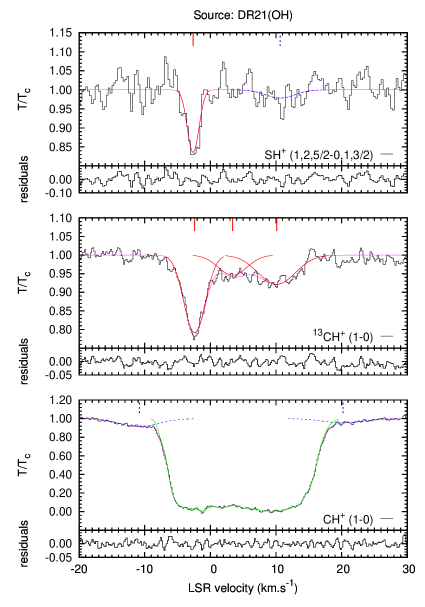
Figure 10: Observational data (black lines) compared to the multi-Gaussian decomposition (purple lines) of the $\rm SH^{+}$ $(1,2,5/2\leftarrow 0,1,3/2)$ (top), $\rm{}^{13}CH^{+}$$(1\leftarrow 0)$ (middle), and $\rm CH^{+}$ $(1\leftarrow 0)$ (bottom) absorption spectra observed towards DR21(OH). The solid red lines and the dashed blue lines correspond to the confirmed (C) and uncertain (U) Gaussian components, respectively (see main text). The solid green lines are the empirical modelling of the $\rm CH^{+}$saturated line profiles.

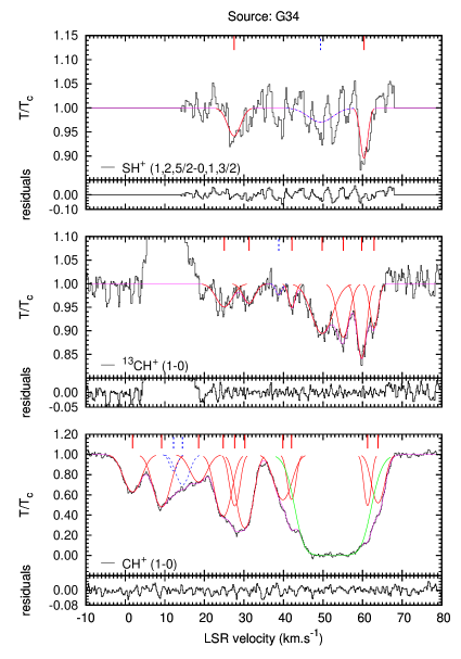
Figure 11: Same as Fig. 10 for the observations towards G34.3+0.1.

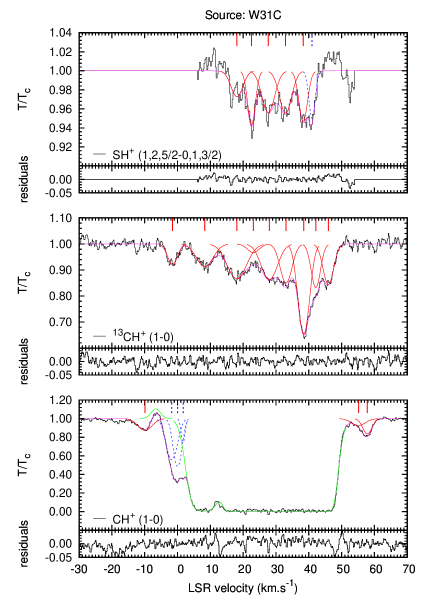
Figure 12: Same as Fig. 10 for the observations towards W31C.

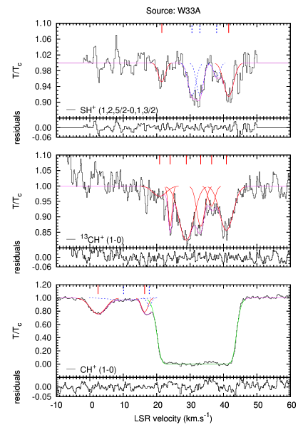
Figure 13: Same as Fig. 10 for the observations towards W33A.

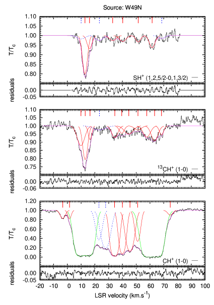
Figure 14: Same as Fig. 10 for the observations towards W49N.

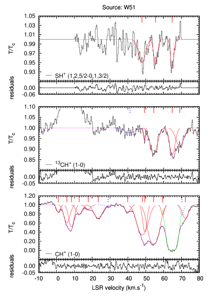
Figure 15: Same as Fig. 10 for the observations towards W51.

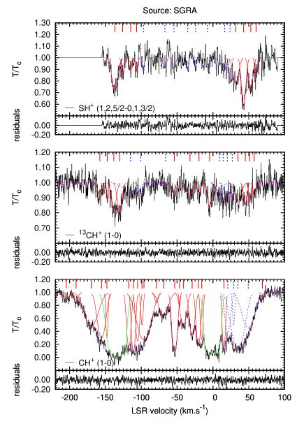
Figure 16: Same as Fig. 10 for the observations towards SgrA*+50.

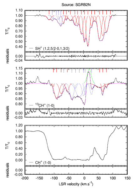
Figure 17: Same as Fig. 10 for the observations towards SgrB2(N).

The results of the Gaussian decomposition procedure applied to the spectra are given in Tables LABEL:TabFit. In turn, Figs. 10 - 17 display the comparison between the result of the fit and the original data, along with the associated residuals. The uncertainties given in the Table LABEL:TabFit are the formal 1-$\sigma$ errors derived from the diagonal elements of the covariance matrix and do not take into account the systematic errors introduced by (1) the finite velocity resolution, (2) the uncertainty on the continuum level, and (3) the error introduced by the decomposition procedure, which depends on its convergence criteria.

According to Godard et al. (2010) (Appendix B), the finite velocity resolution of the spectra introduces an error on the linewidth determination smaller than 8 % for the $\rm CH^{+}$ and $\rm{}^{13}CH^{+}$ components, and smaller than 14 % for the $\rm SH^{+}$ components, if $\Delta\upsilon>1.3$ km s^-1 (the smallest observed linewidth). Furthermore, a relative uncertainty $\epsilon$ on the continuum temperature leads to an error $\delta\tau\sim\epsilon-{\rm ln}(1+\epsilon e^{\tau})$ on the opacity that ranges between 6% and 30 % when $\tau$ varies between 0.03 and 2.7 (the lowest and highest observed central opacities) and using $\epsilon=10$ % (value corresponding to the error on the beam efficiency and the side band ratio, Roelfsema et al. 2012).

Unlike the other numerical fitting methods that are devised to find the global minimum of $\chi^{2}$, the Levenberg Marquardt algorithm is a so-called single-shot method: used when the initial conditions are easily fixed, this algorithm takes advantage of the information on the $\chi^{2}$ derivatives with respect to each parameter to converge on the nearest local minimum. However, since the minimum only corresponds to a statistical estimate of the fit parameters, the code can converge on different solutions close to each other depending on the initial condition, the $\chi^{2}$ valley topography, and the criteria to stop the optimization. To estimate the associated error, we analysed the dispersion of the best-fit solutions when varying the initial conditions: for each spectrum, we assumed an uncertainty of 2 km s^-1 on the initial guess of the positions and the linewidths of the Gaussians. The resulting 4200 fits are found to bracket the optimum solutions given in Table LABEL:TabFit with a standard deviation of 10 % on the central optical depths and the Gaussian linewidths.

When combined, the robustness of the decomposition procedure, the finite resolution, and the uncertainty on the continuum temperature correspond to maximal errors on the calculation of $\Delta\upsilon$ and $\tau$ of 20 % and 30 %, respectively.

Table 5: $\rm CH^{+}$ $(1\leftarrow 0)$, $\rm{}^{13}CH^{+}$ $(1\leftarrow 0)$, and $\rm SH^{+}$ $(1\leftarrow 0)$ absorption line analysis results.

$\rm CH^{+}$ $(1\leftarrow 0)$				$\rm{}^{13}CH^{+}$ $(1\leftarrow 0)$				$\rm SH^{+}$ $(1,2,5/2\leftarrow 0,1,3/2)$
$\upsilon_{0}$	$\Delta\upsilon\pm\sigma(\Delta\upsilon)$	$\tau_{0}\pm\sigma(\tau_{0})$	Va	$\upsilon_{0}$	$\Delta\upsilon\pm\sigma(\Delta\upsilon)$	$\tau_{0}\pm\sigma(\tau_{0})$	Va	$\upsilon_{0}$	$\Delta\upsilon\pm\sigma(\Delta\upsilon)$	$\tau_{0}\pm\sigma(\tau_{0})$	Va
(km s-1)	(km s-1)			(km s-1)	(km s-1)			(km s-1)	(km s-1)
DR21(OH)
-10.8 $\pm$ 0.3	6.9 $\pm$ 0.5	9.1 (-2) $\pm$ 4 (-3)	U	-2.4 $\pm$ 0.1	3.7 $\pm$ 0.1	2.3 (-1) $\pm$ 6 (-3)	C	-2.6 $\pm$ 0.1	2.0 $\pm$ 0.4	1.8 (-1) $\pm$ 3 (-2)	C
20.2 $\pm$ 1.8	7.0 $\pm$ 2.4	4.7 (-2) $\pm$ 1 (-2)	U	3.4 $\pm$ 0.2	5.1 $\pm$ 0.4	5.6 (-2) $\pm$ 4 (-3)	C	10.6 $\pm$ 1.2	5.2 $\pm$ 2.7	2.2 (-2) $\pm$ 2 (-2)	U
				10.1 $\pm$ 0.4	6.6 $\pm$ 0.7	8.2 (-2) $\pm$ 4 (-3)	C
G34
1.8 $\pm$ 0.1	5.0 $\pm$ 0.1	4.6 (-1) $\pm$ 9 (-3)	C	25.0 $\pm$ 0.3	4.8 $\pm$ 0.7	5.1 (-2) $\pm$ 6 (-3)	C	27.5 $\pm$ 0.3	3.8 $\pm$ 0.6	6.2 (-2) $\pm$ 2 (-2)	C
9.2 $\pm$ 0.1	4.6 $\pm$ 0.2	7.3 (-1) $\pm$ 1 (-2)	C	31.3 $\pm$ 0.3	3.5 $\pm$ 0.7	4.2 (-2) $\pm$ 7 (-3)	C	49.4 $\pm$ 0.8	7.3 $\pm$ 2.4	3.3 (-2) $\pm$ 2 (-2)	U
12.2 $\pm$ 0.3	2.2 $\pm$ 0.9	1.8 (-1) $\pm$ 2 (-1)	U	38.8 $\pm$ 0.4	1.7 $\pm$ 0.8	2.4 (-2) $\pm$ 1 (-2)	U	60.4 $\pm$ 0.1	2.2 $\pm$ 0.3	1.1 (-1) $\pm$ 3 (-2)	C
14.5 $\pm$ 0.5	3.7 $\pm$ 1.6	3.6 (-1) $\pm$ 9 (-2)	U	42.1 $\pm$ 0.2	1.9 $\pm$ 0.4	5.2 (-2) $\pm$ 9 (-3)	C
18.5 $\pm$ 0.6	4.7 $\pm$ 0.9	3.2 (-1) $\pm$ 4 (-2)	C	49.8 $\pm$ 0.2	6.2 $\pm$ 0.4	1.1 (-1) $\pm$ 6 (-3)	C
24.8 $\pm$ 0.2	4.2 $\pm$ 0.5	9.5 (-1) $\pm$ 5 (-2)	C	55.1 $\pm$ 0.1	3.5 $\pm$ 0.3	1.2 (-1) $\pm$ 8 (-3)	C
27.7 $\pm$ 0.2	2.7 $\pm$ 0.4	7.1 (-1) $\pm$ 2 (-1)	C	59.8 $\pm$ 0.1	2.8 $\pm$ 0.2	1.7 (-1) $\pm$ 9 (-3)	C
30.2 $\pm$ 0.2	4.0 $\pm$ 0.2	1.3 (+0) $\pm$ 8 (-2)	C	62.9 $\pm$ 0.1	2.3 $\pm$ 0.2	9.9 (-2) $\pm$ 9 (-3)	C
39.8 $\pm$ 0.3	4.8 $\pm$ 0.3	6.0 (-1) $\pm$ 4 (-2)	C
42.0 $\pm$ 0.0	2.3 $\pm$ 0.2	5.9 (-1) $\pm$ 8 (-2)	C
61.3 $\pm$ 0.0	1.9 $\pm$ 0.1	7.1 (-1) $\pm$ 3 (-2)	C
63.9 $\pm$ 0.1	3.5 $\pm$ 0.1	6.5 (-1) $\pm$ 1 (-2)	C
W31C
-9.9 $\pm$ 0.1	5.0 $\pm$ 0.2	1.4 (-1) $\pm$ 4 (-3)	C	-1.5 $\pm$ 0.1	3.5 $\pm$ 0.2	8.2 (-2) $\pm$ 5 (-3)	C	18.1 $\pm$ 0.4	4.2 $\pm$ 1.0	2.7 (-2) $\pm$ 7 (-3)	C
-1.8 $\pm$ 0.8	3.7 $\pm$ 0.6	5.8 (-1) $\pm$ 3 (-1)	U	8.3 $\pm$ 0.2	5.9 $\pm$ 0.4	9.1 (-2) $\pm$ 4 (-3)	C	22.6 $\pm$ 0.2	2.8 $\pm$ 0.4	5.8 (-2) $\pm$ 1 (-2)	C
0.0 $\pm$ 0.2	2.8 $\pm$ 0.5	7.2 (-1) $\pm$ 4 (-1)	U	18.1 $\pm$ 0.2	6.8 $\pm$ 0.5	1.4 (-1) $\pm$ 5 (-3)	C	27.7 $\pm$ 0.5	4.6 $\pm$ 1.3	4.5 (-2) $\pm$ 8 (-3)	C
1.7 $\pm$ 0.1	1.3 $\pm$ 0.2	2.9 (-1) $\pm$ 8 (-2)	U	23.1 $\pm$ 0.4	4.2 $\pm$ 0.8	3.4 (-2) $\pm$ 7 (-3)	C	32.9 $\pm$ 0.4	4.4 $\pm$ 1.3	4.5 (-2) $\pm$ 8 (-3)	C
55.2 $\pm$ 1.6	4.9 $\pm$ 1.6	7.6 (-2) $\pm$ 3 (-2)	C	28.0 $\pm$ 0.2	5.7 $\pm$ 0.4	1.5 (-1) $\pm$ 5 (-3)	C	38.3 $\pm$ 0.4	3.1 $\pm$ 1.0	5.4 (-2) $\pm$ 1 (-2)	C
57.8 $\pm$ 0.2	3.1 $\pm$ 0.4	1.8 (-1) $\pm$ 6 (-2)	C	33.1 $\pm$ 0.1	4.1 $\pm$ 0.2	1.6 (-1) $\pm$ 7 (-3)	C	41.0 $\pm$ 0.3	2.2 $\pm$ 0.5	5.1 (-2) $\pm$ 3 (-2)	U
				38.5 $\pm$ 0.1	3.9 $\pm$ 0.3	4.2 (-1) $\pm$ 1 (-2)	C
				42.1 $\pm$ 0.2	3.2 $\pm$ 0.6	1.8 (-1) $\pm$ 2 (-2)	C
				46.0 $\pm$ 0.2	3.7 $\pm$ 0.3	1.7 (-1) $\pm$ 9 (-3)	C
W33A
2.5 $\pm$ 0.1	5.2 $\pm$ 0.2	2.8 (-1) $\pm$ 1 (-2)	C	20.9 $\pm$ 0.8	4.7 $\pm$ 1.3	4.2 (-2) $\pm$ 1 (-2)	C	21.5 $\pm$ 0.2	2.4 $\pm$ 0.5	4.9 (-2) $\pm$ 1 (-2)	C
10.1 $\pm$ 1.2	8.6 $\pm$ 4.9	3.5 (-2) $\pm$ 5 (-3)	U	24.1 $\pm$ 0.1	1.3 $\pm$ 0.1	1.4 (-1) $\pm$ 1 (-2)	C	30.6 $\pm$ 1.0	2.7 $\pm$ 1.4	8.6 (-2) $\pm$ 7 (-2)	U
16.4 $\pm$ 0.5	2.1 $\pm$ 0.6	2.4 (-1) $\pm$ 6 (-2)	C	28.9 $\pm$ 0.2	5.0 $\pm$ 0.4	1.9 (-1) $\pm$ 7 (-3)	C	32.9 $\pm$ 0.9	2.4 $\pm$ 1.1	8.7 (-2) $\pm$ 9 (-2)	U
17.8 $\pm$ 0.3	1.5 $\pm$ 0.4	1.4 (-1) $\pm$ 1 (-1)	U	33.2 $\pm$ 0.2	2.7 $\pm$ 0.5	1.4 (-1) $\pm$ 1 (-2)	C	38.0 $\pm$ 0.3	2.1 $\pm$ 0.7	3.6 (-2) $\pm$ 2 (-2)	U
				36.5 $\pm$ 0.2	2.3 $\pm$ 0.6	7.0 (-2) $\pm$ 1 (-2)	C	41.6 $\pm$ 0.2	3.4 $\pm$ 0.3	8.9 (-2) $\pm$ 1 (-2)	C
				40.9 $\pm$ 0.1	4.6 $\pm$ 0.3	1.6 (-1) $\pm$ 6 (-3)	C
W49N
-3.4 $\pm$ 0.1	4.1 $\pm$ 0.2	1.9 (-1) $\pm$ 6 (-3)	C	9.9 $\pm$ 0.1	6.2 $\pm$ 0.3	1.3 (-1) $\pm$ 7 (-3)	C	10.0 $\pm$ 1.0	6.3 $\pm$ 2.0	1.8 (-2) $\pm$ 2 (-2)	U
1.6 $\pm$ 0.1	2.8 $\pm$ 0.2	2.0 (-1) $\pm$ 9 (-3)	C	13.0 $\pm$ 0.1	4.1 $\pm$ 0.2	2.3 (-1) $\pm$ 7 (-3)	C	12.8 $\pm$ 0.1	4.0 $\pm$ 0.2	2.2 (-1) $\pm$ 1 (-2)	C
22.9 $\pm$ 0.8	4.8 $\pm$ 0.7	9.9 (-1) $\pm$ 8 (-1)	U	16.5 $\pm$ 0.1	2.9 $\pm$ 0.2	8.8 (-2) $\pm$ 1 (-2)	C	16.1 $\pm$ 0.2	4.0 $\pm$ 0.5	7.2 (-2) $\pm$ 2 (-2)	C
27.8 $\pm$ 0.5	6.5 $\pm$ 4.1	1.7 (+0) $\pm$ 3 (-1)	U	23.3 $\pm$ 1.2	9.9 $\pm$ 2.3	2.5 (-2) $\pm$ 3 (-3)	U	23.3 $\pm$ 0.6	5.8 $\pm$ 1.3	2.6 (-2) $\pm$ 7 (-3)	U
34.3 $\pm$ 0.3	5.2 $\pm$ 1.6	4.0 (+0) $\pm$ 4 (-1)	U	34.5 $\pm$ 0.2	5.1 $\pm$ 0.4	7.5 (-2) $\pm$ 7 (-3)	C	32.9 $\pm$ 0.5	5.4 $\pm$ 1.0	2.7 (-2) $\pm$ 7 (-3)	C
40.0 $\pm$ 0.4	4.6 $\pm$ 1.0	2.7 (+0) $\pm$ 4 (-1)	C	39.5 $\pm$ 0.2	4.1 $\pm$ 0.4	4.7 (-2) $\pm$ 4 (-3)	C	40.2 $\pm$ 0.4	5.5 $\pm$ 0.8	3.1 (-2) $\pm$ 7 (-3)	C
45.5 $\pm$ 0.3	5.8 $\pm$ 0.9	2.1 (+0) $\pm$ 9 (-2)	C	44.6 $\pm$ 0.9	7.3 $\pm$ 1.8	5.2 (-2) $\pm$ 4 (-3)	C	51.5 $\pm$ 0.3	4.0 $\pm$ 0.6	3.4 (-2) $\pm$ 8 (-3)	C
51.1 $\pm$ 0.2	4.1 $\pm$ 0.2	1.1 (+0) $\pm$ 1 (-1)	C	51.3 $\pm$ 0.4	5.8 $\pm$ 0.9	2.6 (-2) $\pm$ 4 (-3)	C	61.6 $\pm$ 0.2	4.7 $\pm$ 0.3	6.5 (-2) $\pm$ 8 (-3)	C
74.7 $\pm$ 0.1	4.1 $\pm$ 0.2	1.1 (-1) $\pm$ 6 (-3)	C	57.7 $\pm$ 0.3	6.0 $\pm$ 0.6	7.2 (-2) $\pm$ 9 (-3)	C	68.6 $\pm$ 0.8	5.2 $\pm$ 1.6	1.5 (-2) $\pm$ 7 (-3)	U
				63.4 $\pm$ 0.3	5.7 $\pm$ 0.5	9.5 (-2) $\pm$ 5 (-3)	C
				68.4 $\pm$ 0.2	3.6 $\pm$ 0.4	5.5 (-2) $\pm$ 6 (-3)	C
W51
1.0 $\pm$ 0.1	2.3 $\pm$ 0.1	1.8 (-1) $\pm$ 9 (-3)	C	41.1 $\pm$ 0.7	7.2 $\pm$ 1.6	2.4 (-2) $\pm$ 5 (-3)	U	47.9 $\pm$ 0.2	4.5 $\pm$ 0.6	5.1 (-2) $\pm$ 1 (-2)	C
5.8 $\pm$ 0.8	3.7 $\pm$ 0.7	5.0 (-1) $\pm$ 2 (-1)	C	49.3 $\pm$ 0.1	1.0 $\pm$ 0.2	5.9 (-2) $\pm$ 1 (-2)	C	55.5 $\pm$ 0.2	2.5 $\pm$ 0.4	5.6 (-2) $\pm$ 2 (-2)	C
8.3 $\pm$ 0.4	3.2 $\pm$ 0.4	6.7 (-1) $\pm$ 2 (-1)	C	54.5 $\pm$ 0.1	4.6 $\pm$ 0.3	1.3 (-1) $\pm$ 6 (-3)	C	64.8 $\pm$ 0.1	2.0 $\pm$ 0.3	6.4 (-2) $\pm$ 2 (-2)	C
12.7 $\pm$ 0.1	3.7 $\pm$ 0.4	2.4 (-1) $\pm$ 8 (-3)	C	64.9 $\pm$ 0.3	3.7 $\pm$ 0.4	1.3 (-1) $\pm$ 2 (-2)	C
17.8 $\pm$ 0.2	3.3 $\pm$ 0.5	1.1 (-1) $\pm$ 8 (-3)	C	69.0 $\pm$ 0.6	5.2 $\pm$ 1.0	8.9 (-2) $\pm$ 9 (-3)	C
23.4 $\pm$ 0.1	5.2 $\pm$ 0.4	3.6 (-1) $\pm$ 7 (-3)	C
28.9 $\pm$ 1.2	4.7 $\pm$ 1.9	3.3 (-2) $\pm$ 1 (-2)	U
39.9 $\pm$ 0.1	3.5 $\pm$ 0.2	1.8 (-1) $\pm$ 7 (-3)	C
48.1 $\pm$ 0.7	6.2 $\pm$ 0.7	1.1 (+0) $\pm$ 2 (-1)	C
49.5 $\pm$ 0.1	2.4 $\pm$ 0.3	8.8 (-1) $\pm$ 2 (-1)	C
54.4 $\pm$ 0.2	5.8 $\pm$ 0.4	2.0 (+0) $\pm$ 1 (-1)	C
59.5 $\pm$ 0.1	1.9 $\pm$ 0.2	2.5 (-1) $\pm$ 3 (-2)	C
70.3 $\pm$ 0.1	2.1 $\pm$ 0.4	2.7 (-1) $\pm$ 1 (-1)	U
72.2 $\pm$ 0.5	3.7 $\pm$ 0.6	3.5 (-1) $\pm$ 5 (-2)	C
SgrA*+50
-204.4 $\pm$ 0.5	8.9 $\pm$ 1.1	1.1 (-1) $\pm$ 1 (-2)	C	-157.9 $\pm$ 0.4	6.4 $\pm$ 0.9	1.0 (-1) $\pm$ 1 (-2)	C	-136.9 $\pm$ 0.2	9.4 $\pm$ 0.5	3.2 (-1) $\pm$ 3 (-2)	C
-191.0 $\pm$ 0.4	6.7 $\pm$ 1.0	1.3 (-1) $\pm$ 2 (-2)	C	-147.4 $\pm$ 0.2	2.1 $\pm$ 0.5	1.3 (-1) $\pm$ 3 (-2)	C	-126.0 $\pm$ 0.3	3.8 $\pm$ 0.6	1.6 (-1) $\pm$ 5 (-2)	C
-169.8 $\pm$ 0.9	20.1 $\pm$ 1.6	7.3 (-1) $\pm$ 2 (-2)	C	-138.3 $\pm$ 0.9	7.5 $\pm$ 1.5	2.0 (-1) $\pm$ 2 (-2)	C	-114.6 $\pm$ 0.4	4.5 $\pm$ 0.9	1.1 (-1) $\pm$ 4 (-2)	C
-155.5 $\pm$ 0.3	11.4 $\pm$ 0.8	1.2 (+0) $\pm$ 7 (-2)	C	-130.3 $\pm$ 0.8	7.3 $\pm$ 1.7	2.0 (-1) $\pm$ 3 (-2)	C	-106.5 $\pm$ 0.4	3.6 $\pm$ 0.8	1.1 (-1) $\pm$ 4 (-2)	C
-147.9 $\pm$ 0.1	3.0 $\pm$ 0.2	1.2 (+0) $\pm$ 8 (-2)	C	-115.0 $\pm$ 2.7	22.7 $\pm$ 10.5	6.7 (-2) $\pm$ 8 (-3)	U	-97.0 $\pm$ 0.3	2.4 $\pm$ 0.6	1.2 (-1) $\pm$ 6 (-2)	U
-117.4 $\pm$ 0.4	5.8 $\pm$ 0.7	1.8 (+0) $\pm$ 1 (-1)	C	-100.7 $\pm$ 0.7	6.9 $\pm$ 2.4	7.4 (-2) $\pm$ 2 (-2)	U	-67.0 $\pm$ 0.6	4.8 $\pm$ 1.4	8.4 (-2) $\pm$ 4 (-2)	U
-110.9 $\pm$ 0.5	5.0 $\pm$ 1.2	2.3 (+0) $\pm$ 3 (-1)	C	-66.0 $\pm$ 1.1	4.4 $\pm$ 2.5	3.3 (-2) $\pm$ 2 (-2)	U	-54.4 $\pm$ 0.5	4.5 $\pm$ 1.1	9.1 (-2) $\pm$ 4 (-2)	U
-105.1 $\pm$ 0.8	5.5 $\pm$ 1.8	1.4 (+0) $\pm$ 4 (-1)	C	-53.7 $\pm$ 0.7	8.8 $\pm$ 1.6	7.8 (-2) $\pm$ 1 (-2)	C	-35.2 $\pm$ 0.3	3.0 $\pm$ 0.7	1.1 (-1) $\pm$ 5 (-2)	U
-98.9 $\pm$ 0.5	3.3 $\pm$ 1.1	7.0 (-1) $\pm$ 2 (-1)	C	-32.0 $\pm$ 0.6	9.0 $\pm$ 1.4	8.9 (-2) $\pm$ 1 (-2)	C	-24.2 $\pm$ 0.3	2.6 $\pm$ 0.8	9.5 (-2) $\pm$ 5 (-2)	U
-96.2 $\pm$ 2.1	19.5 $\pm$ 3.1	1.3 (+0) $\pm$ 1 (-1)	C	-19.4 $\pm$ 0.5	4.7 $\pm$ 1.0	8.3 (-2) $\pm$ 2 (-2)	C	-7.9 $\pm$ 1.0	9.0 $\pm$ 2.2	6.3 (-2) $\pm$ 3 (-2)	U
-78.7 $\pm$ 0.4	5.2 $\pm$ 1.3	1.8 (-1) $\pm$ 5 (-2)	C	-4.7 $\pm$ 0.3	6.3 $\pm$ 0.7	1.8 (-1) $\pm$ 2 (-2)	C	16.4 $\pm$ 2.1	11.7 $\pm$ 4.2	8.3 (-2) $\pm$ 3 (-2)	U
-68.7 $\pm$ 0.4	14.0 $\pm$ 1.3	4.6 (-1) $\pm$ 2 (-2)	C	9.4 $\pm$ 2.5	10.4 $\pm$ 4.9	9.1 (-2) $\pm$ 2 (-2)	U	23.9 $\pm$ 0.5	4.5 $\pm$ 1.3	1.6 (-1) $\pm$ 9 (-2)	U
-53.4 $\pm$ 0.1	6.8 $\pm$ 0.2	2.3 (+0) $\pm$ 9 (-2)	C	14.2 $\pm$ 0.4	2.1 $\pm$ 1.1	8.1 (-2) $\pm$ 4 (-2)	U	31.8 $\pm$ 0.5	8.9 $\pm$ 1.7	2.4 (-1) $\pm$ 4 (-2)	C
-46.4 $\pm$ 0.2	2.2 $\pm$ 0.6	2.5 (-1) $\pm$ 7 (-2)	C	20.1 $\pm$ 1.6	9.0 $\pm$ 4.5	1.1 (-1) $\pm$ 2 (-2)	U	42.9 $\pm$ 0.2	6.5 $\pm$ 0.5	5.3 (-1) $\pm$ 5 (-2)	C
-41.2 $\pm$ 0.3	9.3 $\pm$ 1.0	7.3 (-1) $\pm$ 2 (-2)	C	27.0 $\pm$ 0.3	2.3 $\pm$ 0.9	9.4 (-2) $\pm$ 3 (-2)	U	52.8 $\pm$ 0.2	6.7 $\pm$ 0.8	3.2 (-1) $\pm$ 4 (-2)	C
-28.9 $\pm$ 0.2	7.5 $\pm$ 0.6	1.1 (+0) $\pm$ 3 (-2)	C	34.9 $\pm$ 0.6	10.6 $\pm$ 2.6	1.3 (-1) $\pm$ 1 (-2)	C	60.2 $\pm$ 0.4	3.9 $\pm$ 0.9	1.5 (-1) $\pm$ 5 (-2)	C
-20.2 $\pm$ 0.4	6.1 $\pm$ 0.9	1.6 (+0) $\pm$ 7 (-2)	C	45.3 $\pm$ 0.4	5.5 $\pm$ 1.4	1.5 (-1) $\pm$ 2 (-2)	C
-15.7 $\pm$ 0.3	3.6 $\pm$ 0.3	1.3 (+0) $\pm$ 3 (-1)	C	51.4 $\pm$ 0.4	3.7 $\pm$ 0.9	1.4 (-1) $\pm$ 2 (-2)	C
15.3 $\pm$ 0.2	4.1 $\pm$ 0.3	1.8 (+0) $\pm$ 3 (-1)	C	57.7 $\pm$ 0.4	3.9 $\pm$ 0.9	9.7 (-2) $\pm$ 2 (-2)	C
20.7 $\pm$ 0.8	7.9 $\pm$ 3.2	9.7 (-1) $\pm$ 4 (-1)	U
28.9 $\pm$ 0.3	3.1 $\pm$ 1.1	7.1 (-1) $\pm$ 3 (-1)	U
34.9 $\pm$ 1.6	17.2 $\pm$ 6.0	1.8 (+0) $\pm$ 4 (-1)	U
49.4 $\pm$ 5.6	18.2 $\pm$ 4.4	7.9 (-1) $\pm$ 5 (-1)	U
69.1 $\pm$ 0.5	3.9 $\pm$ 1.2	8.0 (-2) $\pm$ 2 (-2)	C
SgrB2(N)
				-102.0 $\pm$ 0.3	3.6 $\pm$ 0.7	3.3 (-2) $\pm$ 5 (-3)	C	-117.0 $\pm$ 1.4	14.4 $\pm$ 1.4	8.4 (-2) $\pm$ 3 (-2)	C
				-91.5 $\pm$ 0.9	18.0 $\pm$ 1.3	1.6 (-1) $\pm$ 8 (-3)	C	-106.0 $\pm$ 0.3	6.3 $\pm$ 1.2	6.4 (-2) $\pm$ 4 (-2)	U
				-76.0 $\pm$ 0.8	14.1 $\pm$ 3.4	1.1 (-1) $\pm$ 1 (-2)	C	-92.2 $\pm$ 10.6	23.0 $\pm$ 29.7	7.8 (-2) $\pm$ 4 (-2)	U
				-67.2 $\pm$ 0.8	7.0 $\pm$ 2.6	3.2 (-2) $\pm$ 2 (-2)	U	-84.9 $\pm$ 1.3	7.6 $\pm$ 3.2	8.5 (-2) $\pm$ 2 (-1)	U
				-54.8 $\pm$ 1.1	12.4 $\pm$ 2.3	7.4 (-2) $\pm$ 1 (-2)	C	-77.0 $\pm$ 0.4	8.4 $\pm$ 1.6	1.9 (-1) $\pm$ 2 (-1)	U
				-39.4 $\pm$ 2.9	15.5 $\pm$ 4.7	1.6 (-1) $\pm$ 1 (-1)	U	-68.1 $\pm$ 0.7	8.6 $\pm$ 1.3	1.6 (-1) $\pm$ 6 (-2)	C
				-26.9 $\pm$ 0.8	8.4 $\pm$ 4.6	4.9 (-2) $\pm$ 8 (-2)	U	-58.3 $\pm$ 0.2	5.8 $\pm$ 0.6	7.7 (-2) $\pm$ 1 (-2)	C
				-13.9 $\pm$ 10.5	26.5 $\pm$ 56.9	1.4 (-1) $\pm$ 3 (-2)	U	-44.3 $\pm$ 0.6	15.8 $\pm$ 1.7	1.0 (-1) $\pm$ 5 (-3)	C
				0.2 $\pm$ 6.7	11.9 $\pm$ 16.8	1.3 (-1) $\pm$ 4 (-1)	U	-29.1 $\pm$ 0.7	10.8 $\pm$ 1.5	1.8 (-1) $\pm$ 3 (-2)	C
				5.7 $\pm$ 0.8	7.3 $\pm$ 2.7	1.2 (-1) $\pm$ 2 (-1)	U	-20.0 $\pm$ 0.5	9.2 $\pm$ 1.2	1.9 (-1) $\pm$ 5 (-2)	C
				27.4 $\pm$ 1.0	10.6 $\pm$ 2.9	1.1 (-1) $\pm$ 1 (-1)	U	-7.2 $\pm$ 0.2	10.8 $\pm$ 0.6	4.3 (-1) $\pm$ 1 (-2)	C
				55.1 $\pm$ 2.4	31.1 $\pm$ 6.1	3.9 (-2) $\pm$ 2 (-3)	C	3.5 $\pm$ 0.1	8.8 $\pm$ 0.3	6.6 (-1) $\pm$ 3 (-2)	C
				65.7 $\pm$ 0.2	7.7 $\pm$ 0.6	8.5 (-2) $\pm$ 8 (-3)	C	15.3 $\pm$ 0.1	10.6 $\pm$ 0.2	8.7 (-1) $\pm$ 1 (-2)	C
				78.3 $\pm$ 0.4	8.1 $\pm$ 1.6	3.2 (-2) $\pm$ 7 (-3)	C	27.8 $\pm$ 0.2	8.2 $\pm$ 0.5	2.3 (-1) $\pm$ 2 (-2)	C
								38.3 $\pm$ 0.4	11.1 $\pm$ 1.9	1.1 (-1) $\pm$ 9 (-3)	C
								54.8 $\pm$ 0.6	13.3 $\pm$ 1.0	6.0 (-1) $\pm$ 7 (-2)	C
								65.8 $\pm$ 0.5	11.8 $\pm$ 1.1	5.0 (-1) $\pm$ 1 (-1)	C
								79.0 $\pm$ 0.4	13.8 $\pm$ 0.6	3.7 (-1) $\pm$ 2 (-2)	C
								91.9 $\pm$ 0.2	4.3 $\pm$ 0.7	3.6 (-2) $\pm$ 9 (-3)	C
a Validity of the Gaussian detection: C = confirmed if $\Delta\upsilon>3\sigma(\Delta\upsilon)$ and $\tau_{0}>2.5\sigma(\tau_{0})$; U = uncertain otherwise

Table 5: continued.

Appendix B Determination of the excitation temperatures and of the subsequent column densities

The column densities given in Table LABEL:TabIntTau are derived assuming a single excitation temperature $T_{\rm ex}$ for all levels of a given molecule as

$$N=Q(T_{\rm ex})\frac{8\pi\nu_{0}^{3}}{c^{3}}\frac{1}{g_{u}}\frac{1}{A_{ul}}\left[1-e^{-h\nu_{0}/kT_{\rm ex}}\right]^{-1}\int\tau\,d\upsilon$$ (12)

where $\nu_{0}$, $g_{u}$, $g_{l}$ and $A_{ul}$ are the rest frequency, the upper and lower level degeneracies and the Einstein’s coefficients of the observed transition, $Q(T_{\rm ex})$ is the partition funtion, and $c$ is the speed of light.

To derive the $\rm CH^{+}$ and $\rm SH^{+}$ $J=1\leftarrow 0$ line excitation temperatures $T_{\rm ex}$, we adopt the recent computation of the $\rm CH^{+}$ de-excitation rate coefficients by collision with He and $e^{-}$ (Hammami et al. 2009; Lim et al. 1999), and assume a generic $\rm SH^{+}$ de-excitation rate coefficient by collision with H and $\rm H_{2}$ of $10^{-10}$ cm³ s^-1. Because the corresponding critical densities at 100 K, $n_{\rm crit,He}({\rm CH^{+}})\sim 6\times 10^{7}$ $\,{\rm cm}^{-3}$, $n_{{\rm crit},e^{-}}({\rm CH^{+}})\sim 4\times 10^{4}$ $\,{\rm cm}^{-3}$, and $n_{\rm crit,{\rm H_{2}}}({\rm SH^{+}})\sim 7\times 10^{6}$ $\,{\rm cm}^{-3}$, are considerably higher than those of the diffuse ISM, collisions are irrelevant in the excitation of $\rm CH^{+}$ and $\rm SH^{+}$, all the more so collisions of $\rm CH^{+}$ with $\rm H_{2}$ are its destruction pathway. Therefore, the level populations of these two ions only result from radiative excitation and possible additional excitation processes during their chemical formation. Neglecting the latter, we derive the $\rm CH^{+}$ and $\rm SH^{+}$ $J=1\leftarrow 0$ line excitation temperatures $T_{\rm ex}$, from statistical equilibrium, using the submillimetre interstellar radiation field measured at $l=45^{\circ}$ and $b=0^{\circ}$ with the Cosmic Background Explorer (Reach et al. 1995). We obtain low excitation temperatures $T_{\rm ex}(835\,{\rm GHz})=4.4$ K, and $T_{\rm ex}(526\,{\rm GHz})=3.0$ K that agree with the lack of $\rm CH^{+}$ $(2\leftarrow 1)$ and $\rm SH^{+}$ $(21\leftarrow 11)$, $(22\leftarrow 11)$, $(21\leftarrow 10)$, and $(22\leftarrow 12)$ detection in absorption at the velocities of the diffuse medium along the same lines of sight (PRISMAS and HEXOS observations, to be published). Note that an error of about 1 K corresponds to an error on the $\rm CH^{+}$ and $\rm SH^{+}$ column densities smaller than 1 %. While these values of $T_{\rm ex}$ are valid for the velocity components associated with the diffuse interstellar gas, they clearly correspond to lower limits for those associated with the SFRs molecular environments. In the latter case, since the PRISMAS lines of sight target bright IR and submm emitting sources, a complete description of the IR radiative transfer accross the molecular gas surrounding the sources is needed (De Luca et al., in prep.; Vastel et al., in prep.).

For excitation temperatures of ${}^{12,13}{\rm CH^{+}}$ and $\rm SH^{+}$ of 4.4 K and 3.0 K, respectively, Eq. 12 finally becomes

$$N({\rm CH^{+}})=3.11\times 10^{12}\int\tau\,d\upsilon\quad{\rm cm}^{-2},$$ (13)

$$N({\rm{}^{13}CH^{+}})=3.05\times 10^{12}\int\tau\,d\upsilon\quad{\rm cm}^{-2},$$ (14)

and

$$N({\rm SH^{+}})=1.42\times 10^{13}\int\tau\,d\upsilon\quad{\rm cm}^{-2},$$ (15)

using the $\rm CH^{+}$ $J=1\leftarrow 0$, $\rm{}^{13}CH^{+}$ $J=1\leftarrow 0$, and the $\rm SH^{+}$ $N,J,F=1,2,5/2\leftarrow 0,1,3/2$ transitions, respectively.

The $\rm CH^{+}$ line opacity for $N({\rm CH^{+}})=10^{14}$ $\,{\rm cm}^{-2}$ and a linewidth of 4 km s^-1 is of the order of 15 and the expected line emission is about 4 mK (below the noise level, see Tables 1 and 2). The intensities of the $\rm{}^{13}CH^{+}$ and $\rm SH^{+}$ lines that are optically thin are even lower.

Appendix C Tracers of molecular hydrogen in the diffuse ISM

The methylidyne radical CH has often been used as a probe of molecular hydrogen because of its linear relation with $\rm H_{2}$ observed in the local diffuse medium (Federman 1982) and in dark clouds (Mattila 1986). Compiling the UV and visible data obtained on 48 lines of sight (Savage et al. 1977; Rachford et al. 2002; Crane et al. 1995; Crawford 1995; Allen 1994; Gredel et al. 1993; Federman et al. 1994; Danks et al. 1984; Jenniskens et al. 1992), Liszt & Lucas (2002) derived a mean ratio ${N({\rm CH})}/{N({\rm H}_{2})}\sim 4.3\times 10^{-8}$, while Sheffer et al. (2008) found ${N({\rm CH})}/{N({\rm H}_{2})}\sim 3.5\times 10^{-8}$, using their observations of the absorption profiles of $\rm H_{2}$ and CH on a sample of 90 diffuse clouds. Although the latter could be used in this work to estimate $N({\rm H}_{2})$, based on the Herschel observations of the six hyperfine components of the CH $J=1/2-3/2$ absorption line (Gerin et al. 2010b), it raises several problems that have to be taken into account.

• As quoted by Liszt & Lucas (2002) and Sheffer et al. (2008), there is a significant scatter (a dispersion of about a factor of 3) on the ${N({\rm CH})}-{N({\rm H}_{2})}$ relation observed in the local diffuse medium, up to ${N({\rm H}_{2})}=10^{21}$ cm^-2.

• Despite the similarity of the CH absorption profiles with those of other tracers of molecular hydrogen (PRISMAS observations, to be published), a ${N({\rm CH})}-{N({\rm H}_{2})}$ correlation has never been directly measured in the inner Galactic ISM.

• Crane et al. (1995) and Lambert et al. (1990) found that the linewidths of CH observed in absorption are highly variable from one diffuse cloud component to another. They reported the detection of CH line profiles either similar to or more Gaussian and less broad than those of $\rm CH^{+}$. This result was then confirmed by Pan et al. (2005), who divided their observed CH absorption features into two categories: those with CN-like and those with $\rm CH^{+}$-like line profiles. This implies that the production of CH in the interstellar medium can sometimes be linked to the production of $\rm CH^{+}$and depends only slightly on the molecular hydrogen abundance (Godard et al., in prep.).

For these reasons, we derive the $\rm H_{2}$ column densities from observations of the $J=1\leftarrow 0$ ground-state rotational transition of hydrogen fluoride (HF) performed with the Herschel/HIFI instrument. If HF is saturated or not available, $\rm H_{2}$ is deduced from CH, assuming a mean HF/CH abundance ratio of 0.4 (see columns 5 and 6 of Table LABEL:TabHI). The absorption line analysis performed by Neufeld et al. (2010b) and Sonnentrucker et al. (2010) showed that (1) the HF profiles are similar to those of $\rm H_{2}O$, and (2) HF accounts for more than 30 % of the total fluorine nuclei in the gas-phase along these sight-lines. Since both results agree with the chemical models that predict that the production of HF does not depend on the dynamics of the gas and that HF is the main F-bearing species, we deduce the ${N({\rm HF})}-{N({\rm H}_{2})}$ relation from an analytical study of the fluorine chemistry. For the range of parameters defining the diffuse and transluscent gas (Snow & McCall 2006), $10<{n_{\rm H}}<5000{\,{\rm cm}^{-3}}$, $0<A_{V}<5$, and ${n({\rm CO})}/[{\rm C}]<0.9$, the abundance of HF is driven by only four chemical reactions (Neufeld & Wolfire 2009) :

$$\begin{array}[]{l l l l l l l l}{\rm F}&+&{\rm H}_{2}&\rightarrow&{\rm HF}&+&{\rm H}&\qquad(k_{1}),\\ {\rm HF}&+&\gamma&\rightarrow&{\rm F}&+&{\rm H}&\qquad(\zeta_{\rm HF}),\\ {\rm HF}&+&{\rm C}^{+}&\rightarrow&{\rm CF}^{+}&+&{\rm H}&\qquad(k_{2}),\,\,{\rm and}\\ {\rm CF}^{+}&+&{\rm e}^{-}&\rightarrow&{\rm F}&+&{\rm C}&\qquad(k_{3}),\\ \end{array}$$ (16)

where

$$\begin{array}[]{l l l}k_{1}&=&1.00\times 10^{-10}\,\,[{\rm exp}(-450{\rm K}/T)+0.078\,{\rm exp}(-80{\rm K}/T)\\ &&+0.0155\,{\rm exp}(-10{\rm K}/T)]\,\,{\rm cm}^{3}{\rm s}^{-1},\\ \zeta_{\rm HF}&=&1.17\times 10^{-10}\,\,{\rm exp}(-2.2A_{V})\,\,{\rm s}^{-1},\\ k_{2}&=&7.20\times 10^{-09}\,\,(T/300K)^{-0.15}\,\,{\rm cm}^{3}{\rm s}^{-1},\,\,{\rm and}\\ k_{3}&=&5.20\times 10^{-08}\,\,(T/300K)^{-0.80}\,\,{\rm cm}^{3}{\rm s}^{-1}\end{array}$$ (17)

are their respective reaction rate coefficients from the calculations and laboratory measurements (Zhu et al. 2002; Brown & Balint-Kurti 2000; Neufeld et al. 2005; Novotny et al. 2005). Therefore, assuming that there is no depletion of F on interstellar dust, and that the carbon is fully ionized and the sole source of electrons, the HF and $\rm H_{2}$ abundances are related by

$$\frac{n({\rm HF})}{n({\rm H}_{2})}=\frac{\left[{\rm F}\right]}{\big{(}\left[{\rm C}\right]k_{2}+\zeta_{\rm HF}/n_{\rm H}\big{)}/k_{1}+1/2f_{{\rm H}_{2}}\big{(}1+k_{2}/k_{3}\big{)}},$$ (18)

where $\left[{\rm F}\right]$ and $\left[{\rm C}\right]$ are the fluorine and carbon elemental gas phase abundances relative to H nuclei (assumed to equal those observed in the solar neighbourhood, $\sim 1.8\times 10^{-8}$ and $\sim 1.4\times 10^{-4}$ respectively, Savage & Sembach 1996; Sofia & Meyer 2001; Snow et al. 2007), ${n_{\rm H}}$ is the gas density, and $f_{{\rm H}_{2}}$ is the molecular fraction defined as $f_{{\rm H}_{2}}=2n({\rm H}_{2})/n_{\rm H}$. For ${n_{\rm H}}>30$ $\,{\rm cm}^{-3}$ and $A_{V}>0.2$, because F reacts rapidly with $\rm H_{2}$, the left-hand side of the denominator of Eq. 18 can be neglected, more than 90 % of the interstellar fluorine being in HF and less than 10 % in $\rm CF^{+}$. We thus assume a ${n({\rm HF})}/{n({\rm H}_{2})}$ abundance ratio of $3.6\times 10^{-8}$.

Although HF is preferred to CH here as a tracer of molecular hydrogen, relation 18 has to be used cautiously because: (1) it has never been proven observationally, (2) this abundance ratio linearly depends on the fluorine elemental abundance, which can vary with the Galactocentric distance (Daflon & Cunha 2004; Rudolph et al. 2006; Abia et al. 2010), and (3) it also depends on the depletion of fluorine onto grains, which can become important in the molecular gas. We note that the $\rm H_{2}$ molecular fraction computed as $2N({\rm H_{2}})/{N_{\rm H}}$ on the velocity intervals given in Table LABEL:TabHI ranges between 0.05 and 1 with an average value of $\sim 0.4$ (Neufeld et al., in prep.). While this value suggests that the diffuse medium sampled by $\rm CH^{+}$, $\rm{}^{13}CH^{+}$, and $\rm SH^{+}$ is on average weakly molecular, it does not preclude the existence within this gas of regions where $f_{{\rm H_{2}}}=1$. A complete analysis of HF and CH as tracers of molecular hydrogen will be performed by Godard et al. (in prep).