Comparing Mid-Infrared Globular Cluster Colors With Population Synthesis Models

Abstract

Several population synthesis models now predict integrated colors of simple stellar populations in the mid-infrared bands. To date, the models have not been extensively tested in this wavelength range. In a comparison of the predictions of several recent population synthesis models, the integrated colors are found to cover approximately the same range but to disagree in detail, for example on the effects of metallicity. To test against observational data, globular clusters are used as the closest objects to idealized groups of stars with a single age and single metallicity. Using recent mass estimates, we have compiled a sample of massive, old globular clusters in M31 which contain enough stars to guard against the stochastic effects of small-number statistics, and measured their integrated colors in the Spitzer/IRAC bands. Comparison of the cluster photometry in the IRAC bands with the model predictions shows that the models reproduce the cluster colors reasonably well, except for a small (not statistically significant) offset in $[4.5]-[5.8]$. In this color, models without circumstellar dust emission predict bluer values than are observed. Model predictions of colors formed from the $V$ band and the IRAC 3.6 and 4.5 µm bands are redder than the observed data at high metallicities and we discuss several possible explanations. In agreement with model predictions, $V-[3.6]$ and $V-[4.5]$ colors are found to have metallicity sensitivity similar to or slightly better than $V-K_{s}$.

1 Introduction

Star clusters are popular probes of the history of galaxy and star formation. As compact systems with relatively homogeneous properties, their stellar and dynamical histories can be modeled with reasonable accuracy, at least compared to their parent galaxies. Studies of extragalactic star clusters have experienced a major step forward with the availability of the Hubble Space Telescope, which provided the spatial resolution necessary to identify clusters in distant galaxies and resolve those in nearby galaxies into individual stars, and large ground-based telescopes, which provide the light-gathering power to study these faint objects spectroscopically. The study of extragalactic GCs has provided important clues to the process of galaxy assembly and complements the direct study of high-redshift galaxies (Brodie & Strader, 2006).

Star clusters also provide important tests of simple stellar population (SSP) models constructed via population synthesis methods. Although the evidence is now overwhelming that globular clusters are not single-age, single-metallicity populations as previously believed (see the review by Bragaglia, 2010), they are still less complex than the population mix found in even the smallest galaxies. As such, they provide important observational tests for population synthesis models, and there have been many examples of such tests (Peacock et al., 2011; Riffel et al., 2010; Conroy & Gunn, 2010; Pessev et al., 2008; Barmby & Huchra, 2000; Bica & Alloin, 1986). Although becoming increasingly important in the study of nearby stellar populations (e.g. Sheth et al., 2010), and having the advantage of reduced extinction sensitivity, the model predictions at mid-infrared wavelengths $\lambda\gtrsim 3$ $\mu$m, have not been well-tested. Mid-infrared observations from ground-based telescopes are impractical for all but the brightest sources, due to the high background, and the existing stellar libraries may not yet be adequate (although see Vandenbussche et al., 2002; Sloan et al., 2003; Hodge et al., 2004). The ATLAS9 model atmospheres, on which many population synthesis models are at least partly based, have line opacity spectra calculated to a maximum wavelength of 10 µm. Modeling infrared stellar spectra with a Rayleigh-Jeans law is quite common (e.g. Zasowski et al., 2009), but this is “clearly a crude approximation” (Marigo et al., 2008). Those authors state that bolometric corrections for the coolest stars are uncertain by up to a few tenths of a magnitude. In their investigation on the use of model atmospheres for infrared calibration, Decin & Eriksson (2007) found that model spectra are accurate to 3% in the mid-IR but also noted that “for the purpose of calculating theoretical spectra in the mid to far-IR, some line lists are still far from complete or accurate”.

The Spitzer Space Telescope probes these mid-infrared wavelengths. While young star clusters have been the subject of numerous investigations with Spitzer (e.g. Gutermuth et al., 2009), there has been relatively little analysis of the mid-infrared properties of old star clusters. Old star clusters’ declining spectral energy distribution in the mid-infrared, in combination with the presumed lack of interesting spectral features, is presumably the reason for this lack of attention. Mid-infrared observations have been used in studies of mass-losing stars in individual clusters (Boyer et al., 2006, 2008, 2010; Origlia et al., 2007, 2010) as well as searches for cold dust in the intracluster medium (Matsunaga et al., 2008; Barmby et al., 2009). One of the few studies of extragalactic globular cluster systems is that of Spitler et al. (2008). The present paper provides mid-infrared photometry of massive globular clusters in the Andromeda galaxy, M31 (catalog ), taken with the Spitzer Space Telescope, and compares them to population synthesis models which predict magnitudes in the IRAC bands, namely GALEV (Kotulla et al., 2009), FSPS (Conroy et al., 2009) and models from the Padova group (Marigo et al., 2008). Only the four IRAC bands are used here. M31 clusters are generally too faint to be detected in the MIPS observations of Gordon et al. (2005), and photometry of the handful of Milky Way clusters observed with the MIPS instrument is published elsewhere (Boyer et al., 2006, 2008; Barmby et al., 2009).

Throughout this work we use the Vega magnitude system and assume a distance to M31 of 780 kpc (McConnachie et al., 2005), for which 1″ corresponds to 3.78 pc.

2 Data and Models

2.1 Cluster Mass Limit

Star clusters contain a limited number of stars and photometry of star clusters must consider stochastic effects (Buzzoni, 1989; Renzini, 1998). The integrated light of a cluster can be dominated by a few bright stars, particularly in the infrared where the luminosity of the asymptotic giant branch is highest (Fouesneau & Lançon, 2010). For this first comparison of star cluster photometry with SSP models in the mid-infrared, we wanted to avoid stochastic effects as much as possible, so we sought to select only the most massive clusters. One criterion for choosing a selection limit is the lowest luminosity limit (LLL) defined by Cerviño & Luridiana (2004). This limit is defined for a specific SSP model as the luminosity of the brightest star included in the model, at the age, metallicity, and wavelength under consideration. For 10 Gyr old clusters, Cerviño & Luridiana (2004) found the total mass corresponding to the LLL in the $K$-band to be approximately $10^{5}$ M_☉; those authors showed that a total mass of about 10 times this limit is required in order for stochastic effects to cause less than a 10% dispersion in the total luminosity.

Related to the LLL approach is the concept of the “effective number of stars” emitting at a given wavelength, introduced by Buzzoni (1989). With $N_{\rm eff}$ defined via $\delta L_{\rm tot}/L_{\rm tot}=N_{\rm eff}^{-1/2}$, the value of $N_{\rm eff}$ for a 10% uncertainty in luminosity is $N_{\rm eff}=(0.1)^{-2}=100$. For a 10% color uncertainty, assuming the same $N_{\rm eff}$ for both bands, $N_{\rm eff}\geq 200$ (Buzzoni, 2005). The Evolutionary Population Synthesis (EPS) website tabulates model predictions of $N_{\rm eff}(\lambda)$ as a function of age for populations with $L_{\rm bol}=10^{10}L_{\sun}$. For ages of 10–15 Gyr, typical values of $N_{\rm eff}(4\,\mu{\rm m})$ range from $10^{6.6}-10^{6.85}$ depending on the metallicity, IMF and horizontal branch treatment; for ages of 5 Gyr, $N_{\rm eff}(4\,\mu{\rm m})\sim 10^{6.4}$. To scale $N_{\rm eff}$ from $L_{\rm bol}=10^{10}L_{\sun}$ to a fixed mass, we used the $M/L_{\rm bol}$ tabulated by the EPS models. For $[{\rm M/H}]=-1.27$, a typical value for the globular clusters under consideration, $N_{\rm eff}$ values for a $10^{6}$ M_☉ population are 300 (15 Gyr), 270 (10 Gyr), and 260 (8 Gyr). These suggest that clusters with masses of $10^{6}$ M_☉ should not have their integrated mid-IR photometry strongly affected by stochastic effects, while clusters with mass $10^{5}$ M_☉ would have $N_{\rm eff}$ well below the requirements. We used this result to set our lower mass limit at $10^{6}$ M_☉.

2.2 Cluster Sample Selection

For this first comparison between SSP models and star cluster colors, we wanted to remove age as a variable if possible, and select only old clusters. The clusters we considered all belong to the Milky Way, M31, or the LMC. While many other Local Group dwarf galaxies have a few globular clusters each (see the compilation by Forbes et al., 2000), the few available estimates of those clusters’ masses in the literature show the largest of them to have masses about $10^{5}$ M_☉. M33 has numerous star clusters, with a recent catalogue given by Sarajedini & Mancone (2007); however it has few truly old clusters, and few clusters with mass estimates comparable to those available in other galaxies. For Milky Way globular clusters we take the inclusion of a cluster in the catalog of Harris (2010) to mean that its age is $\gtrsim 10$ Gyr. For LMC clusters we considered only clusters classified as having ages $>10$ Gyr by Pessev et al. (2008); these ages were compiled from the results of color-magnitude diagram (CMD) fitting. Age determination for M31 clusters is more difficult, and, with one exception (Brown et al., 2004), CMD-fitting ages from the main sequence turnoff are not available. Perina et al. (2011) noted that deriving M31 cluster ages from integrated spectroscopy can be problematic. They found that two clusters previously suspected to be of intermediate age based on integrated spectra had blue horizontal branches and were likely of comparable age to the oldest Galactic GCs. They also found significant differences between ages determined from spectral energy distribution (SED) fitting and the CMD analysis. With the caveat that ages from spectroscopy may be unreliable, a uniform determination of ages for the M31 GCs reduces scatter due to mixing of different methods, and we use the values by Caldwell et al. (2011) as the basis for selecting our sample. These were derived by comparing Lick indices from integrated spectroscopy to the SSP models of Schiavon (2007). An important limitation of this analysis is that ages could not be determined for clusters with metallicities ${\rm[Fe/H]}\lesssim-1$. It is possible that some younger clusters could be lurking in the sample, although we considered only M31 clusters that had not been identified as young by any previous work.

There are a number of methods for estimating the total mass of a star cluster. While velocity dispersions either from integrated spectra or spectra of individual stars provide the most direct measurements of the gravitational potential of a cluster, such measurements are not available for many Local Group star clusters, particularly in M31 which has the largest population. A more widely-applicable method involves measuring the total luminosity and multiplying by a mass-to-light ratio. Total luminosity can be measured by either large-aperture photometry or fitting and extrapolation of a surface brightness profile. For M31 clusters, a comprehensive set of mass estimates is available in the work of Caldwell et al. (2011), who estimated masses by multiplying reddening-corrected $V$-band luminosities (from Caldwell et al., 2009) by $M/L_{V}=2$. With the goal of selecting a uniform sample, we used these mass estimates exclusively to select the final M31 sample; a few additional outlying clusters for which masses were not given by Caldwell et al. (2011) but which have mass estimates in their online catalog (G001, B358, MGC-1, B468, B293) were also included. For Milky Way and LMC clusters, we used near-infrared $K_{s}$-band magnitudes as given by Cohen (2006) and Pessev et al. (2006, 2008). The near-infrared is often used as an indicator of stellar mass in studies of external galaxies since it is expected to be dominated by low-mass stars and is not strongly sensitive to recent star formation (Bell & de Jong, 2001). The clusters’ magnitude were converted to luminosities using $M_{\sun,Ks}=3.29$ (Blanton & Roweis, 2007) and multiplied by $(M/L)_{K_{s}}=0.9$ in solar units, the lower end of the range quoted for single-metallicity populations by Maraston (2005). We also considered cluster masses derived from fitting of optical surface brightness profiles by McLaughlin & van der Marel (2005); these masses are primarily derived from $V$-band observations (corrected for extinction) and assume $(M/L)_{V}=2$ (McLaughlin, 2000). Some Milky Way clusters (particularly core-collapse candidates) are missing from the McLaughlin & van der Marel (2005) database.

We combined the two methods to select a final list of massive Local Group globular clusters. Excluding the anomalous cluster $\omega$ Cen, only a handful of Milky Way clusters have masses $>10^{6}$ M_☉: NGC 104 (catalog ), NGC 6388 (catalog ), NGC 6441 (catalog ), and NGC 6715 (catalog ). A further 8 Milky Way clusters (NGC 2808 (catalog ), NGC 7089 (catalog ), NGC 2419 (catalog ), NGC 6266 (catalog ), NGC 6273 (catalog ), NGC 6356 (catalog ), NGC 6402 (catalog ), NGC 6440 (catalog )) and two Magellanic Cloud clusters (NGC 1835 (catalog ), NGC 1916 (catalog )) had masses likely to be above $5\times 10^{5}$ M_☉. But nearly all of the massive Local Group globular clusters belong to M31, a total of 58 objects. After examining the available Spitzer/IRAC data for Milky Way and LMC clusters, we eventually decided against using data on those galaxies’ GCs in our analysis: the Milky Way cluster data had technical issues (long frametimes and in-place repeats) as well as only covering a single $5\arcmin\times 5\arcmin$ field of view in all four IRAC bands. The LMC clusters NGC 1916 is located near a region of diffuse emission, making background subtraction for this cluster extremely difficult. IRAC photometry of a larger sample of LMC clusters has been reported by Pessev et al. (2010).

2.3 IRAC Observations and Photometry

The M31 bulge and some of the brightest M31 clusters had individual deep Spitzer/IRAC observations as part of PID 3400 (PI M. Rich). These images also include a number of additional clusters fortuitously located near the target clusters. The data were taken with 30-second frame times, 22 dither positions with 4 frames per position, and so have overall depths of about 40 minutes per sky position. Saturation limits for IRAC images with these frametimes are in the range $8<m_{\rm Vega}<11$ (Spitzer Science Center, 2010). The brightest GCs in M31 have $K_{s}\sim 11$ (Galleti et al., 2004), so saturation of the clusters was not expected to be an issue. We retrieved the data from the Spitzer Heritage Archive and used the post-BCD mosaics as produced by versions 18.7 and 18.18 of the pipeline.

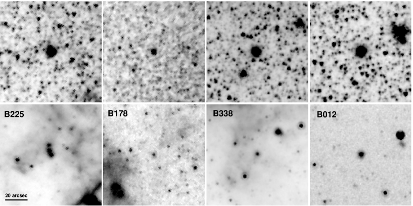
Figure 1: IRAC 3.6µm (top) and 8.0µm (bottom) images of M31 globular clusters. All images are 90″ square with north up and east to the left. The clusters range from $K_{s}\sim 11.5$ (B225) to $K_{s}\sim 13.3$ (B178). The left two panels show clusters in the shallow M31 mosaic (PID 3126) while the right two panels show clusters observed in deeper images (PID 3400).

The main observational dataset for the M31 clusters comprises the IRAC mosaics taken as part of program PID 3126, described in Barmby et al. (2006). In brief, the observations cover a total area of about $3\fdg 7\times 1\fdg 0$ along the major axis of M31, with an extension to include NGC 205. The central portion of the disk was covered to a depth of six 12-second frames per position, and the outer area by four 30-second frames per position. The mosaics used for this analysis are improved versions of the mosaics used by Barmby et al. (2006) and are described by Mould et al. (2008). Of the 58 clusters in our list of massive M31 globulars, 11 were imaged in all four bands in the deep PID3400 data, 41 were imaged only on the shallow M31 mosaics, two objects (B405, MGC-1) had no IRAC images available, and 3 objects (B240, B381, B383) were at the edge of the mosaic image and had only noisy data in 4.5 and 8.0 µm available. Cluster B095 is located about 7″ from a much brighter star and is contaminated by detector artifacts due to the star; we judged that obtaining reliable photometry in the IRAC bands was not possible. The final sample of M31 clusters analyzed here therefore has a total of 52 members. Sample IRAC images of M31 globular clusters are shown in Figure 1.

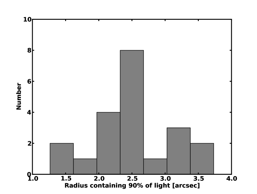
Figure 2: Distribution of $R_{90}$—the radius containing 90% of the integrated light, in projection— for M31 globular clusters.

The typical half-light radius of an M31 GC is $R_{h}\sim 3$ pc, or about 0.75″ (Peacock et al., 2010; Barmby et al., 2007). While this is smaller than the full-width at half-maximum of the IRAC point spread function (PSF), it is large enough that M31 GCs appear slightly resolved (see Figure 1). Aperture photometry is thus more appropriate for these objects than PSF-fitting photometry. But how do we best account for the different PSF in the different IRAC bands, and decide which aperture should be used? From the point of view of capturing all of the light from a cluster, a large aperture is desirable. Use of ‘total’ magnitudes also facilitates comparison between widely-separated wavelength regimes, where not only the PSF but the apparent cluster structure, may differ (see Cohen, 2006, for a discussion of the subtleties in aperture-matching). However, the use of a large aperture would result in low signal-to-noise in 5.8 and 8.0 $\mu$m  bands, where the clusters are faint and the background bright. Using smaller apertures has the problem that the different PSF results in aperture corrections that are not the same in all bands.

To deal with the aperture issues, we took two approaches to photometry of the M31 clusters. To compute IRAC-only colors, we computed aperture magnitudes in a relatively small apertures, and dealt with the variable PSF by convolving the images in the 3.6, 4.5, and 5.8 $\mu$m  bands to the 8.0 $\mu$m  resolution. (A similar approach was used by Clemens et al., 2009, in their study of near-to-mid-infrared colors of Coma cluster galaxies.) For colors which combine the 3.6 and 4.5 $\mu$m  bands with visible-light or near-infrared bands, we measured ‘total’ IRAC magnitudes in a standard large aperture. Convolution was done using the IRAF fconvolve task and the convolution kernels described by Gordon et al. (2008). For the clusters observed as part of the large mosaics, we extracted $2.5\arcmin\times 2.5\arcmin$ ‘postage stamp’ images and convolved these, rather than attempting to convolve the original mosaics. We compared aperture photometry on the original and convolved deep images to show that the convolution performed as expected: the median difference in aperture magnitudes between convolved and unconvolved images was close to the difference between aperture corrections between the convolved band and the 8.0 $\mu$m  band as tabulated in the IRAC Instrument Handbook (Spitzer Science Center, 2010). To choose a small aperture size, we used the results of surface brightness profile fitting from Hubble Space Telescope images of M31 globular clusters (Barmby et al., 2007) to compute $R_{90}$, the projected radius containing 90% of the integrated light, for each cluster. Figure 2 shows the distribution of $R_{90}$ for the 34 clusters from our sample analyzed by Barmby et al. (2007). The median of the $R_{90}$ distribution is 2$\farcs$5, with a maximum of 3$\farcs$7. These values refer to the intrinsic profile before convolution with the HST PSF; the effects of the Spitzer/IRAC PSF are more significant and mean that $R_{90}$ as observed in IRAC images will be larger. To maximize signal-to-noise and still include a significant fraction of cluster light, we chose one of the standard IRAC aperture sizes, a radius of 3$\farcs$66.

Aperture photometry was performed using the IRAF/APPHOT package. Flux was measured in circular apertures of radii 3$\farcs$66 (and 12$\farcs$2 for the 3.6 and 4.5 $\mu$m  bands only), with background measured in an annulus of inner and outer radii 3$\farcs$6–8$\farcs$5 (14$\farcs$6–24$\farcs$4) subtracted. This background annulus for the small aperture is the smaller of two tabulated in the Instrument Handbook. We used it because a few clusters had nearby diffuse emission which could bias the background estimate in a larger annulus. We verified that in most cases the choice of background annulus had no effect on the resulting photometry. Calibration to the Vega system was made using the Vega IRAC-band flux densities given by the Spitzer Science Center. Uncertainties on the photometric measurements were estimated using the formula in apphot/phot, with a correction to the background noise term which accounts for the correlated noise introduced by pixel re-sampling during mosaicing. As the background variation is by far the dominant source of noise in these measurements, this is an important correction. Table 1 gives the photometry. We checked the internal consistency of the photometry by comparing measurements of the same clusters on the deep and shallow IRAC images. There is some scatter between the two image types, but magnitude offsets are consistent with zero. In the 4 IRAC bands, the offsets are (mean $\pm$ standard deviation): $-0.03\pm 0.04,-0.06\pm 0.08,-0.06\pm 0.07,-0.06\pm 0.09$.

2.4 2MASS Photometry and Extinction Correction

While globular clusters have not been extensively observed in the mid-infrared, there is a long history of using them to test population synthesis models in the near-infrared, so it is of interest to connect these two regimes. The most widely-used near-infrared photometric system is that of 2MASS (Skrutskie et al., 2006), and the 2MASS data on M31 GCs has been examined by Galleti et al. (2004) and Nantais et al. (2006). Peacock et al. (2010) also presented observations of M31 GCs in the $K_{s}$ band based on deeper UKIRT imaging. We chose to re-measure the M31 GC magnitudes on the 2MASS ‘6x’ Atlas images because the observations of Peacock et al. (2010) only covered 60% of our cluster sample, the compilation of Galleti et al. (2004) used the original shallow 2MASS images of M31, and the compilation of Nantais et al. (2006) used the 2MASS Point Source Catalog, which might be inappropriate for the larger M31 clusters. To maintain consistency with the colors measured using the IRAC data, we retrieved 2MASS images of the M31 GCs and used these to measure aperture magnitudes with the same large photometric and background apertures used for the IRAC data. We chose to use the large apertures rather than trying to match the spatial resolution between IRAC and 2MASS because the temporal variation in the 2MASS PSF makes any such matching significantly more complicated. The photometric uncertainties were estimated using the same procedure as for the IRAC magnitudes, which is based on the procedure detailed in section 8av of the 2MASS All-Sky Data Release Explanatory Supplement. Table 1 gives the 2MASS $K_{s}$ photometry. We compared our aperture photometry with the total magnitudes measured on UKIRT images by Peacock et al. (2010). The UKIRT magnitudes are slightly fainter, with the median offset $0.08\pm 0.09$ mag. This is not too surprising, since we used an aperture slightly larger than most of the apertures used by Peacock et al. (2010). It could result in our ‘total’ $K_{s}$ magnitudes being slightly too bright; however for the purposes of computing 2MASS-to-IRAC colors this effect should cancel out.

While extinction has a much smaller effect on photometry in the mid-infrared than in visible-light or even the near-infrared, the effect is not completely negligible. The exact shape of the extinction law in the mid-infrared appears to vary with position in the Galaxy (Indebetouw et al., 2005; Román-Zúñiga et al., 2007; Flaherty et al., 2007; Nishiyama et al., 2009; Gao et al., 2009) but all of these analyses agree that the extinction at IRAC wavelengths is greater than would be expected from a power-law extrapolation of the near-infrared extinction curve. In the analysis that follows, we correct the cluster colors for extinction using the $E(B-V)$ values given by Caldwell et al. (2011). These values include both foreground extinction and extinction internal to M31. For this analysis we use the bandpass-averaged extinction values of Indebetouw et al. (2005), as tabulated in Gao et al. (2009): $A_{3.6}/A_{K_{s}}=0.56$ and $A_{\lambda}/A_{K_{s}}=0.43$ for the other three IRAC bands. We assume $A_{K_{s}}/E(B-V)=0.35$ (Cambrésy et al., 2002) and the standard $A_{V}/E(B-V)=3.1$.

2.5 Population Synthesis Models

While there are numerous population synthesis models currently available — two of the most widely-used being Bruzual & Charlot (2003) and Maraston (2005) — to our knowledge only three models give explicit predictions for magnitudes in the IRAC bandpasses. These are GALEV (Kotulla et al., 2009), FSPS (Conroy et al., 2009; Conroy & Gunn, 2010), and the SSP models provided by the Padova group through their STEL webserver (Marigo et al., 2008; Girardi et al., 2010, hereafter referred to as ‘Padova’). While many other models can be used to generate predicted IRAC magnitudes from spectral energy distributions, using three model families suffices for this first analysis. These models contain some of the same input ingredients but differ in other ways, such as the treatment of thermally-pulsing asymptotic giant branch and horizontal branch stars. GALEV also provides chemically consistent modeling of galaxies while the other two do not, although this difference is not relevant for the present study.

Population synthesis models have mostly focused on the visible-light regime, so it is reasonable to ask what the input ingredients of these models are in the infrared. The treatment of red giant and asymptotic giant branch stars is expected to be particularly important, since these evolutionary stages dominate the light of old populations, especially in the near-infrared (Buzzoni, 1989; Maraston, 2005, and many others). All three models were consider here use Padova isochrones, so an important factor in any different outputs is the stellar libraries. GALEV and FSPS both use the BaSeL stellar libraries: version 2.2 for GALEV (Lejeune et al., 1998) and version 3.1 (Westera et al., 2002) for FSPS. BaSeL is based mainly on the stellar atmosphere models of Kurucz (1992), but those models do not include the coolest stars, so BaSeL also includes model M giant atmospheres from Fluks et al. (1994) and Bessell et al. (1989, 1991). The Padova SSP models use some of the same input ingredients—newer ATLAS models from Castelli & Kurucz (2003) and the Fluks et al. (1994) models—but without going through the BaSeL library. Since the Fluks et al. (1994) models extend to wavelengths up to 12.5µm and the Bessell et al. (1989, 1991) models only to 4.1µm, we can infer that the former models provide the basis for the predictions tested here; however, this is not explicitly stated in any of the model descriptions. The thermally-pulsing asymptotic giant branch can also be an important contributor to the integrated light of star clusters (Maraston, 2005), although it is not expected to be important at globular cluster ages. For these stars, FSPS uses empirical spectra from Lançon & Mouhcine (2002) while the Padova models use synthetic spectra from Loidl et al. (2001). Both the Lançon & Mouhcine (2002) and Loidl et al. (2001) spectra extend only to 2.5 µm. The Padova models extend the AGB spectra beyond 2.5 $\mu$m  with a Rayleigh-Jeans model: FSPS extrapolates carbon star spectra with Aringer et al. (2009) synthetic spectra. Kotulla et al. (2009) did not describe any special treatment of TP-AGB stars in GALEV.

For all three models, we generated predicted SSP colors in the 2MASS and IRAC bands for a Salpeter (1955) ($0.1-100$ M_☉) initial mass function and ages from 1 Gyr up to the oldest available. We retrieved SSP predictions from the online GALEV interface using all available fixed metallicity values ${\rm[M/H]}=\log(Z/Z_{\sun})=(-1.7,-0.7,-0.3,0.0,+0.3)$. For FSPS, we used version 2.3 of the code to generate predicted magnitudes for simple stellar populations with metallicity values ${\rm[M/H]}=(-1.68,-0.69,-0.30,0.0,+0.20)$. The default options for other parameters were used. For the Padova models, we used metallicities of ${\rm[M/H]}=(-1.68,-0.70,-0.30,0.0,+0.20)$, with the default parameters: evolutionary tracks from Marigo et al. (2008), with the Girardi et al. (2010) case A correction, and no circumstellar dust (although see below). For all models, no intrinsic dust extinction was applied. We interpolated the GALEV magnitudes to ${\rm[M/H]}=+0.2$ so that all three models represented the same five metallicity values. These metallicity values adequately cover the range of metallicities for clusters in the present sample ($-1.9\leq{\rm[M/H]}\leq-0.1$); although M31 has lower-metallicity clusters (Caldwell et al., 2011), they are not present among the most massive objects.

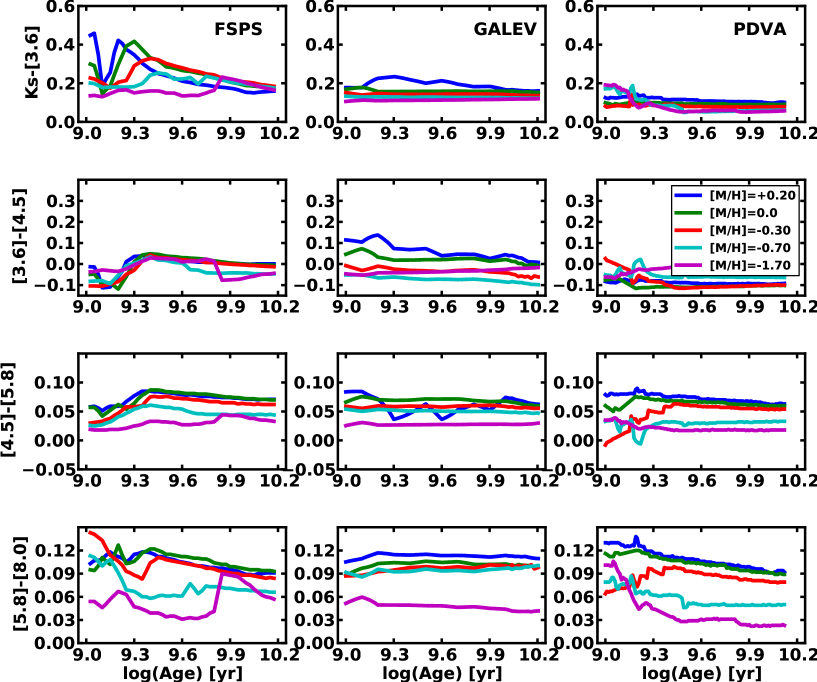
Figure 3: Predicted IRAC colors from three population synthesis models, as a function of simple stellar population age. Left column: FSPS Conroy et al. (2009), center column: GALEV (Kotulla et al., 2009), right column: Padova (Marigo et al., 2008). The same set of metallicities is plotted for all 3 models.

Figure 3 shows predicted colors from the models as functions of age. At old ages, all models show a rather small range of predicted mid-infrared colors, only a few tenths of a magnitude. Although the colors mostly become slightly bluer with age, the size of this effect is very small. There are some systematic differences in the models’ predictions, with, in general, the FSPS models predicting the greatest color variations over the displayed age range. While there is general agreement that higher metallicities result in redder colors within a model family, the different models do not agree on either the size of this effect or its location. For example, the FSPS $K_{s}-[3.6]$ color for the most metal-poor model is redder than the same color for the most metal-rich Padova model. Each of the models has at least one metallicity track that behaves differently from others in the same family, but which metallicity is the outlier changes depending on the color and model family. Since all three models use the same set of isochrones, the difference in predicted colors must be due to some other factor. One likely contributor is the different spectral libraries used for post-main-sequence stars. Another could be numerical issues surrounding the stability of integration over short-lived, but luminous stages (Maraston, 2005; Tinsley & Gunn, 1976).

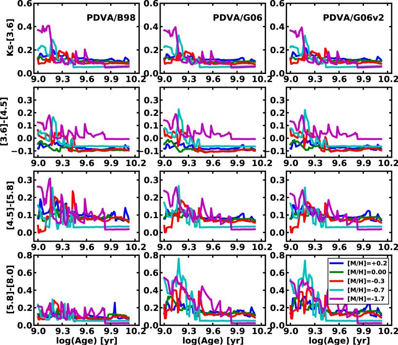
Figure 4: Predicted IRAC colors from Padova population synthesis models, as a function of simple stellar population age. The 3 columns show colors resulting from 3 different options for circumstellar dust: B98 is Bressan et al. (1998), G06 is Groenewegen (2006) 100% AlO_x for M stars and 100% amorphous carbon for C stars, and G06v2 is Groenewegen (2006) 60% silicate/40% AlO_x for M stars and 85% amorphous carbon/15% SiC for C stars.

While Milky Way globular clusters have not shown evidence for intracluster dust (Matsunaga et al., 2008; Barmby et al., 2009), mid-infrared observations have provided important evidence for dust in the envelopes of individual mass-losing stars (Boyer et al., 2010; Origlia et al., 2010). So it is reasonable to ask what the effects of dusty mass loss would be on the integrated mid-infrared colors of a clusters. The Padova models can optionally include these effects for stars with significant mass loss: red supergiants, TP-AGB, and upper-RGB stars (see Marigo et al., 2008, for details). Figure 4 shows the result of adding circumstellar dust to the Padova simple stellar populations. This figure shows the Padova models with three different prescriptions for circumstellar dust: silicate dust for M stars and carbon-rich dust for C stars (Bressan et al., 1998), 100% AlO_x for M stars and 100% amorphous carbon for C stars, and 60% silicate/40% AlO_x for M stars and 85% amorphous carbon/15% SiC for C stars (the latter two both from Groenewegen, 2006). Comparing with the right panel of Figure 3 shows that including circumstellar dust emission causes the colors to vary more with age (all of the Padova models are plotted with the same time resolution) and become redder, particularly at the longer wavelengths. These effects are stronger for ages $\lesssim 8$ Gyr: models at the oldest ages are close in color to the non-circumstellar-dust version. In most cases, the choice of circumstellar dust prescription does not have a large effect on the predicted colors. The exception is $[5.8]-[8.0]$ where the Bressan et al. (1998) prescription results in bluer colors, particularly at lower metallicity, than either of the two prescriptions from Groenewegen (2006). To maintain compatibility with the other two families, the dusty circumstellar models are not shown in the comparison with the cluster data, but these effects will be considered in the discussion.

3 Analysis and Discussion

3.1 Cluster color distributions

Before comparing to models, the most basic analysis of the globular cluster colors is to examine their distribution. Figure 5 shows the distribution of the four colors constructed with bandpasses adjacent in wavelength. Overplotted are Gaussians normalized to the same area, with the data-derived means and standard deviations: $K_{s}-[3.6]=0.13\pm 0.11$, $[3.6]-[4.5]=-0.04\pm 0.05$, $[4.5]-[5.8]=0.09\pm 0.07$ and $[5.8]-[8.0]=0.09\pm 0.12$ (mean $\pm$ standard deviation). Pahre et al. (2004) gave theoretical colors of M0 III stars in the IRAC bands of $[3.6]-[4.5]=-0.15$, $[4.5]-[5.8]=+0.11$ and $[5.8]-[8.0]=+0.04$. The mean colors of the cluster sample are formally consistent with the naive expectation of zero magnitudes, and in the longer wavelengths with the theoretical colors. The mean $[3.6]-[4.5]$ color of the clusters is slightly redder than the expected giant color, as are the model colors described in Section 3.2, so we suggest that there may be a problem with the value given by Pahre et al. (2004). The $[3.6]-[4.5]$ color shows the narrowest color distribution, unsurprising since these two bands have the most similar PSF and do not suffer from any possible aperture-matching problems between 2MASS and IRAC data. At the longer wavelengths, where the clusters are fainter and the background brighter, the observational uncertainties are larger. Contributions by diffuse PAH emission could also skew the 5.8 and 8.0 µm fluxes, although this should be minimized by the close-in background aperture used for photometry.

As Figure 3 shows, the expected range of mid-infrared colors for old stellar populations is rather small, a few tenths of a magnitude. Are the distributions that we measure the result of a single intrinsic color, broadened by observational uncertainty? One argument against this is that, for the IRAC-only colors, the standard deviations of the color distributions are broader than the average photometric uncertainties, by factors of 1.5–2.5. Applying the D’Agostino-Pearson normality test to all four color distributions, we can reject the hypothesis of normality in the $[3.6]-[4.5]$ and $[5.8]-[8.0]$ colors, but not in $K_{s}-[3.6]$ or $[4.5]-[5.8]$. We also compared the color distributions to Gaussians with zero mean and standard deviation given by the average photometric uncertainty using a Kolmorgorov-Smirnov test. In all cases the hypothesis that the observed distributions were drawn from the zero-mean distribution was rejected. We conclude that the cluster colors have some intrinsic spread and that the observed distributions are not merely delta functions broadened by observational uncertainty. Mis-estimates of reddening should have only a small effect on colors derived from adjacent band and are unlikely to cause significant scatter. A spread in ages is a possible reason for a color distribution spread; this is discussed further in Section 3.2. Another possible explanation is that the relatively poor spatial resolution of IRAC leads to contamination of some clusters’ colors by sources nearby in the M31 disk.

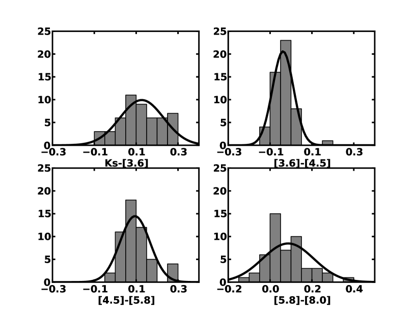
Figure 5: Distribution of near- and mid-infrared extinction-corrected colors for massive M31 globular clusters. Gaussians with mean and standard deviation computed from the data are overplotted for reference.

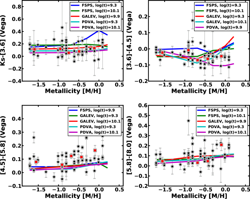
Figure 6: Near and mid-infrared colors (corrected for extinction) as a function of metallicity for massive M31 globular clusters (points) and SSP model predictions (lines). Each of the model prediction lines represents one model family at a specific age between 2 and 12.5 Gyr. Solid black symbols are individual M31 clusters; open symbols (red in the online version) represent the luminosity-weighted mean colors of clusters in quintiles of metallicity.

3.2 Observed and model colors

While, by design, the M31 clusters in our sample cover a fairly small range in mass, they do cover a range of about 2 dex in metallicity. Comparing models to cluster colors as a function of metallicity allows us to see how the ranges of the data and models coincide. Figure 6 shows these comparisons for the same colors as shown in Figure 5. The models plotted are a subset of those shown in Figure 3, chosen to represent the range of model colors for ages of 2, 8, and 12.5 Gyr. For metallicity values of the clusters, we used the spectroscopic ${\rm[Fe/H]}$ measurements of Caldwell et al. (2011) and converted to total metallicity with ${\rm[M/H]}={\rm[Fe/H]}+0.94[\alpha/{\rm Fe}]$ (Thomas et al., 2003). Beasley et al. (2005) found a large spread in the degree of $\alpha$-element enhancement for M31 clusters; we use a typical value of $[\alpha/{\rm Fe}]=0.2$. As well as data for individual clusters, the Figure also shows the luminosity-weighted mean colors of clusters grouped in quintiles of metallicity. In general, the clusters cover a wider range of color than do the models, but the models typically fall within the range of the cluster data. The reddest model in the $K_{s}-[3.6]$ and $[3.6]-[4.5]$ plots is the FSPS 2 Gyr model, which does not appear to be a good fit to the data; however, the 2 Gyr Padova model does match the data in $K_{s}-[3.6]$, as does the 2 Gyr GALEV model in $[3.6]-[4.5]$. The observational scatter in these two colors is large enough that older models are also broadly consistent with the data.

At the longer IRAC wavelengths, the range of model colors is very small and the models are generally in good agreement with each other. In $[4.5]-[5.8]$, the cluster mean colors are slightly redder than all of the models by up to 0.1 mag, but the offset is statistically significant in only two of the five metallicity bins. The scatter of some objects to redder colors could be due to systematic effects in the photometry (incomplete background subtraction, failure to completely match apertures with the convolution method), or, more interestingly, it could indicate that some clusters’ colors are affected by circumstellar dust emission. In $[5.8]-[8.0]$, the mean cluster colors are generally in agreement with the models except possibly at the highest metallicity. For the most part, the redder colors predicted by the Padova models for stars with circumstellar dust do not appear to match the cluster data. This lends support to the idea that these clusters are truly old objects and their infrared light is not dominated by emission from circumstellar dust.

Optical to near-infrared colors (e.g., $V-K_{s}$) are good metallicity indicators in old stellar populations, because they are sensitive to the temperature of the red giant branch. Optical-to-mid-infrared colors have been less well studied. Spitler et al. (2008) measured $V-[3.6]$ for GCs in NGC 5128 and NGC 4594 and found that this color showed a good correlation with spectroscopic metallicity. To see if the same is true for M31 GCs, we computed optical-to-mid-infrared colors using the $V$-band photometry tabulated by Caldwell et al. (2009), corrected for extinction using the $E(B-V)$ values given by Caldwell et al. (2011). These colors are much more sensitive to reddening than the infrared-only colors considered above. Caldwell et al. (2011) estimated the typical reddening uncertainty to be 0.1 mag: changing a reddening estimate by this much would correspond to a change of nearly 0.3 mag in reddening-corrected $V-K_{s}$.

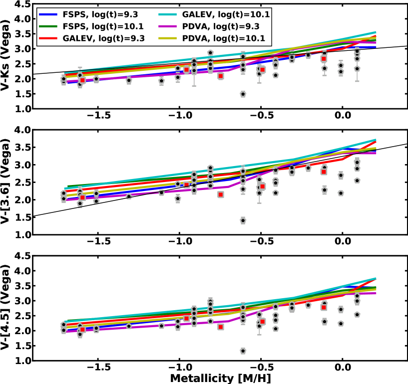
Figure 7: Optical to near/mid-infrared colors (corrected for extinction) as a function of metallicity for massive M31 globular clusters (points) and SSP model predictions (thick lines). Thin lines in the top two panels are fits of $V-K_{s}$ against metallicity for Milky Way clusters from Cohen et al. (2007) and $V-[3.6]$ against metallicity for GCs in NGC 5128 and NGC 4594 from Spitler et al. (2008). Symbols as in Figure 6; error bars on the data points do not include uncertainties due to reddening correction, which could be up to 0.3 mag. The very blue cluster at ${\rm[M/H]}=-0.6$ is B037, a cluster with a large ($E(B-V)\gtrsim 1.3$) and highly uncertain reddening (Caldwell et al., 2011; Barmby et al., 2002).

Figure 7 shows the $V-K_{s}$, $V-[3.6]$ and $V-[4.5]$ colors as a function of metallicity for M31 GCs. Overplotted are the relations predicted by the GALEV, FSPS, and Padova models (ages 2 and 12 Gyr), as well as fits to the color-metallicity relationships for other GC systems: $V-K_{s}$ for Milky Way clusters from Cohen et al. (2007) and $V-[3.6]$ from Spitler et al. (2008). In all three model families, older models are redder at a given metallicity than younger models. There is a significant spread in predicted color with metallicity: the GALEV models are almost always redder than the Padova models at a given metallicity, with the FSPS models intermediate. The Figure shows that the models do not predict a strictly linear color-metallicity relation for any of the colors; particularly for $V-[3.6]$ and $V-[4.5]$, all of the models show a slight change in slope at $[M/H]=-0.7$. The empirical fit in $V-K_{s}$ captures the model behavior reasonably well, although as noted by Conroy & Gunn (2010), the models are redder than the data at high metallicities. In $V-[3.6]$, the fit matches the models well at high metallicities but is bluer than the models at low metallicities. Spitler et al. (2008) found the same result, although interestingly they were comparing to a completely different set of models.

The cluster data points plotted in Figure 7 are bluer than the models except at the lowest metallicities. A problem with the photometry does not provide an immediate explanation. Since our large-aperture IR magnitudes could slightly overestimate the clusters’ brightness (because of contamination by nearby objects), our photometry seems more prone to make the clusters too red, rather than too blue. A number of other systematic effects could come into play:

1. One possibility is that our method of using the average $\alpha$-element abundances to compute ${\rm[M/H]}$ is too simplistic, although the ${\rm[M/H]}$ values would have to change drastically to make the data points compatible with the models.

2. Another possibility is that the clusters are much younger than expected and should therefore be compared to younger models. We think this is unlikely: deriving ages from mid-IR model predictions and colors alone (clearly a risky idea given the limited age sensitivity shown in Figure 3) would suggest ages younger than 2 Gyr. Such young ages would have a substantial effect on optical and near-infrared colors, and there are no suggestions from recent spectroscopic or SED-fitting studies of M31 clusters (e.g. Rey et al., 2007; Caldwell et al., 2009; Wang et al., 2010) that the brightest clusters are all so young.

3. Reddening corrections could play a role: the metal-rich clusters have a higher average reddening than the metal-poor clusters, so if the $E(B-V)$ estimates of Caldwell et al. (2011) were too high, the corrected colors of metal-rich clusters would be more strongly affected. As an example, we found that reducing the reddening values of all clusters by 20% brought the data points and models into better agreement over the entire metallicity range.

4. All three model families could have some common flaw in the spectral libraries that causes them to predict too much infrared flux, or too little $V$-band. Some SSP models are known to have problems reproducing globular cluster colors in the infrared (Conroy & Gunn, 2010, Figure 6), so a problem with the less-well-calibrated IRAC bands seems plausible.

5. Finally, the results of Strader et al. (2009) on the mass-to-light ratios for M31 clusters suggest an interesting alternative. Those authors found $M/L$ to be lower for metal-rich M31 clusters than for metal-poor clusters, contrary to predictions from SSP models. While younger populations are expected to have lower $M/L$, Strader et al. argued against the metal-rich M31 clusters being even intermediate-age, and concluded that variations in the cluster mass function, either initially or through dynamical evolution, were more likely explanations. A flatter mass function, required to match the mass-to-light ratios, should qualitatively also result in bluer predicted colors: fewer low-mass stars would mean less $V$-band light (dominated by the main sequence), and more high-mass stars should mean more infrared light (dominated by giants). The different initial mass functions available in the SSP models do not result in large differences in predicted colors, but perhaps more drastic alterations to the mass function would change colors more dramatically.

We consider the last three of these options to be more plausible explanations of the offset. Distinguishing between them requires better-quality data than are currently available.

If we assume that the model-data offset in $V-$infrared colors is due to a systematic problem in the models, we can still use our data to explore the metallicity sensitivity of these colors. We performed least-squares fits of color as a function of metallicity, weighted by the color uncertainty. For the clusters binned in metallicity, we found slopes in the range 0.42–0.46 for all three colors, very close to the value of 0.409 derived by Cohen et al. (2007) for $V-K_{s}$ in Milky Way globular clusters. For the full, unbinned M31 sample we derive a slope of 0.39 for $V-K_{s}$. For this sample we derive somewhat steeper slopes of 0.68 for $V-[3.6]$ and 0.59 for $V-[4.5]$, still shallower than the slope of 0.90 derived by Spitler et al. (2008), although those authors were fitting the reverse function (metallicity as a function of color). The steeper slopes for the unbinned data agree better with the general trend of the models. Of course, there is no guarantee that a linear fit is the correct representation of the actual physical situation (and see Yoon et al., 2006), but the scatter visible in Figure 7 indicates that a more complicated fit is not likely to be meaningful.

The slopes of the linear fits indicate that $V-{\rm IRAC}$ colors could be a useful metallicity indicator for simple stellar populations. The low infrared background seen by Spitzer means that IRAC observations to comparable depth can be made much more quickly than ground-based near-infrared observations; however compared to $V-K_{s}$, $V-{\rm IRAC}$ colors have the disadvantage of being somewhat more sensitive to reddening uncertainties and having (typically) poorer spatial resolution. Echoing Spitler et al. (2008), we caution that these colors are not well-calibrated for super-solar or very low ($[M/H]\lesssim-1.9$) metallicities. Using the M31 clusters to calibrate the relation would require careful matching of apertures in photometric bands differing by almost a factor of 10 in wavelength (see Cohen et al., 2007, for a description of the difficulties involved in matching just between visible and near-infrared) and is not a trivial task even for these bright clusters. Using more distant, unresolved clusters to calibrate the visible-to-IRAC color/metallicity relation might be a better approach.

4 Summary

We have presented mid-infrared photometry of massive globular clusters in M31, in order to test the color predictions of population synthesis models. To our knowledge, this is the first such test of the models in all four IRAC bands. The three different model families discussed here differ somewhat in their predicted colors and in the systematic effects of age and metallicity. As might be expected, models including circumstellar dust emission predict redder colors, particularly at longer wavelengths, and more color variability with age, particularly for ages $\lesssim 8$ Gyr. Except for the $[5.8]-[8.0]$ color, the exact choice of circumstellar dust prescription does not make a substantial difference. The present level of observational precision does not permit distinguishing between models; the considerable observational uncertainties, especially at the longer wavelengths, are due to the bright background from the galaxy and the falling cluster spectral energy distribution. Within these uncertainties, the data and models are mostly in agreement. We find a small but not statistically significant offset between models and data in the $[4.5]-[5.8]$ color; if real, this could be an indication of emission from circumstellar dust in some clusters. Finally, we find that visible-to-IRAC colors are bluer than model predictions, for reasons which are unclear. These colors could still be feasible metallicity indicators for simple stellar populations but further work is required to establish accurate calibrations.

Facilities: Spitzer (IRAC), FLWO:2MASS ()

Table 1: IRAC photometry for massive M31 globular clusters

Name	3$\farcs$66 radius aperture				12$\farcs$2 radius aperture			${\rm[Fe/H]}$	$E(B-V)$
	[3.6]	[4.5]	[5.8]	[8.0]	$K_{s}$	[3.6]	[4.5]
B006	$12.90\pm 0.01$	$12.97\pm 0.01$	$12.89\pm 0.02$	$12.81\pm 0.02$	$12.43\pm 0.03$	$12.27\pm 0.01$	$12.32\pm 0.01$	$-0.5$	0.17
B012	$12.99\pm 0.01$	$13.00\pm 0.01$	$12.91\pm 0.01$	$12.89\pm 0.01$	$12.70\pm 0.04$	$12.67\pm 0.01$	$12.60\pm 0.01$	$-1.7$	0.17
B017	$12.85\pm 0.01$	$12.80\pm 0.01$	$12.78\pm 0.01$	$12.63\pm 0.02$	$12.44\pm 0.04$	$12.36\pm 0.01$	$12.30\pm 0.01$	$-0.8$	0.47
B019	$12.17\pm 0.01$	$12.28\pm 0.01$	$12.21\pm 0.01$	$12.13\pm 0.02$	$11.93\pm 0.03$	$11.70\pm 0.01$	$11.79\pm 0.01$	$-0.8$	0.22
B023	$11.03\pm 0.01$	$11.11\pm 0.01$	$10.95\pm 0.01$	$10.91\pm 0.01$	$10.73\pm 0.01$	$10.59\pm 0.01$	$10.67\pm 0.01$	$-0.7$	0.42
B027	$13.23\pm 0.01$	$13.26\pm 0.01$	$13.29\pm 0.03$	$13.28\pm 0.04$	$13.16\pm 0.12$	$12.85\pm 0.04$	$12.89\pm 0.03$	$-1.3$	0.19
B034	$12.74\pm 0.01$	$12.77\pm 0.01$	$12.67\pm 0.02$	$12.67\pm 0.03$	$12.37\pm 0.06$	$12.09\pm 0.01$	$12.12\pm 0.01$	$-0.6$	0.16
B037	$11.20\pm 0.01$	$11.25\pm 0.01$	$11.12\pm 0.01$	$11.02\pm 0.01$	$10.94\pm 0.02$	$10.74\pm 0.01$	$10.79\pm 0.01$	$-0.8$	1.61
B051	$13.07\pm 0.01$	$13.14\pm 0.01$	$13.05\pm 0.02$	$13.12\pm 0.04$	$12.49\pm 0.05$	$12.35\pm 0.01$	$12.38\pm 0.01$	$-0.8$	0.38
B055	$12.86\pm 0.02$	$12.85\pm 0.02$	$12.57\pm 0.03$	$12.05\pm 0.03$	$12.34\pm 0.09$	$11.98\pm 0.02$	$11.90\pm 0.02$	$-0.1$	0.54
B058	$12.76\pm 0.01$	$12.71\pm 0.01$	$12.76\pm 0.02$	$12.65\pm 0.04$	$12.33\pm 0.05$	$12.15\pm 0.01$	$12.14\pm 0.01$	$-1.1$	0.15
B061	$13.16\pm 0.01$	$13.20\pm 0.01$	$13.10\pm 0.02$	$13.04\pm 0.03$	$12.90\pm 0.08$	$12.58\pm 0.02$	$12.61\pm 0.02$	$-0.7$	0.49
B063	$12.18\pm 0.01$	$12.26\pm 0.01$	$12.10\pm 0.01$	$11.98\pm 0.01$	$11.92\pm 0.03$	$11.75\pm 0.01$	$11.82\pm 0.01$	$-0.8$	0.49
B068	$12.91\pm 0.01$	$12.94\pm 0.01$	$12.84\pm 0.02$	$12.76\pm 0.04$	$12.56\pm 0.13$	$12.23\pm 0.02$	$12.20\pm 0.02$	$-0.2$	0.45
B082	$11.64\pm 0.01$	$11.66\pm 0.01$	$11.58\pm 0.01$	$11.50\pm 0.02$	$11.38\pm 0.09$	$11.19\pm 0.01$	$11.20\pm 0.01$	$-0.7$	0.94
B086	$12.95\pm 0.03$	$13.02\pm 0.03$	$12.76\pm 0.03$	$12.64\pm 0.05$	$12.63\pm 0.26$	$12.47\pm 0.10$	$12.71\pm 0.10$	$-1.8$	0.13
B088	$12.50\pm 0.01$	$12.49\pm 0.01$	$12.47\pm 0.01$	$12.36\pm 0.02$	$12.12\pm 0.04$	$11.96\pm 0.01$	$11.96\pm 0.01$	$-1.8$	0.53
B091D	$12.29\pm 0.03$	$12.41\pm 0.03$	$12.32\pm 0.03$	$12.20\pm 0.04$	$\cdots$	$\cdots$	$\cdots$	$-0.7$	0.24
B094	$12.70\pm 0.01$	$12.74\pm 0.01$	$12.65\pm 0.02$	$12.44\pm 0.04$	$12.22\pm 0.05$	$12.06\pm 0.01$	$12.11\pm 0.01$	$-0.4$	0.22
B096	$13.19\pm 0.03$	$13.28\pm 0.04$	$13.27\pm 0.04$	$13.30\pm 0.13$	$12.54\pm 0.23$	$12.50\pm 0.09$	$12.46\pm 0.07$	$-0.3$	0.63
B103	$12.20\pm 0.03$	$12.27\pm 0.02$	$12.18\pm 0.03$	$12.03\pm 0.06$	$11.46\pm 0.17$	$11.30\pm 0.01$	$11.43\pm 0.01$	$-0.5$	0.34
B107	$13.25\pm 0.04$	$13.07\pm 0.03$	$13.05\pm 0.06$	$12.92\pm 0.13$	$12.59\pm 0.29$	$12.32\pm 0.10$	$12.16\pm 0.08$	$-1.0$	0.22
B116	$12.84\pm 0.01$	$12.85\pm 0.01$	$12.76\pm 0.02$	$12.72\pm 0.04$	$12.35\pm 0.04$	$12.17\pm 0.01$	$12.19\pm 0.01$	$-0.6$	0.72
B124	$11.70\pm 0.10$	$11.72\pm 0.09$	$11.47\pm 0.10$	$11.41\pm 0.11$	$\cdots$	$\cdots$	$\cdots$	$-0.5$	0.17
B131	$12.81\pm 0.09$	$12.79\pm 0.08$	$12.60\pm 0.09$	$12.34\pm 0.11$	$\cdots$	$\cdots$	$\cdots$	$-0.7$	0.18
B135	$13.33\pm 0.01$	$13.34\pm 0.01$	$13.22\pm 0.02$	$13.16\pm 0.04$	$13.05\pm 0.10$	$12.98\pm 0.03$	$12.95\pm 0.03$	$-1.8$	0.28
B143	$13.03\pm 0.05$	$13.14\pm 0.05$	$12.94\pm 0.05$	$12.75\pm 0.06$	$12.71\pm 0.41$	$12.44\pm 0.01$	$12.44\pm 0.01$	$-0.1$	0.34
B148	$13.52\pm 0.08$	$13.51\pm 0.08$	$13.49\pm 0.11$	$13.04\pm 0.09$	$12.78\pm 0.46$	$12.27\pm 0.04$	$12.34\pm 0.04$	$-1.1$	0.28
B151	$11.57\pm 0.01$	$11.65\pm 0.01$	$11.46\pm 0.01$	$11.39\pm 0.02$	$11.20\pm 0.05$	$11.03\pm 0.01$	$11.14\pm 0.01$	$-0.6$	0.53
B163	$11.90\pm 0.01$	$11.97\pm 0.01$	$11.86\pm 0.01$	$11.68\pm 0.01$	$11.50\pm 0.03$	$11.32\pm 0.01$	$11.40\pm 0.01$	$-0.1$	0.21
B171	$12.35\pm 0.01$	$12.35\pm 0.01$	$12.25\pm 0.01$	$12.02\pm 0.02$	$11.90\pm 0.07$	$11.79\pm 0.03$	$11.79\pm 0.02$	$-0.3$	0.19
B174	$12.79\pm 0.01$	$12.86\pm 0.01$	$12.79\pm 0.02$	$12.76\pm 0.03$	$12.33\pm 0.05$	$12.18\pm 0.01$	$12.26\pm 0.02$	$-1.0$	0.28
B178	$12.90\pm 0.01$	$12.91\pm 0.01$	$12.84\pm 0.02$	$12.71\pm 0.03$	$12.65\pm 0.12$	$12.64\pm 0.05$	$12.54\pm 0.05$	$-1.2$	0.10
B179	$13.05\pm 0.02$	$13.08\pm 0.02$	$13.08\pm 0.03$	$12.86\pm 0.07$	$12.67\pm 0.17$	$12.53\pm 0.06$	$12.37\pm 0.05$	$-1.0$	0.10
B182	$12.74\pm 0.01$	$12.83\pm 0.02$	$12.71\pm 0.03$	$12.63\pm 0.06$	$12.16\pm 0.04$	$11.84\pm 0.01$	$11.84\pm 0.01$	$-1.0$	0.33
B185	$12.84\pm 0.01$	$12.88\pm 0.01$	$12.79\pm 0.02$	$12.75\pm 0.04$	$12.54\pm 0.09$	$12.49\pm 0.04$	$12.61\pm 0.04$	$-0.6$	0.21
B193	$12.43\pm 0.01$	$12.48\pm 0.01$	$12.36\pm 0.01$	$12.16\pm 0.02$	$12.03\pm 0.05$	$11.77\pm 0.01$	$11.66\pm 0.01$	$-0.1$	0.23
B206	$12.78\pm 0.02$	$12.76\pm 0.02$	$12.75\pm 0.03$	$12.62\pm 0.03$	$12.19\pm 0.06$	$12.15\pm 0.02$	$12.13\pm 0.02$	$-1.1$	0.10
B212	$13.42\pm 0.01$	$13.45\pm 0.01$	$13.36\pm 0.02$	$13.35\pm 0.04$	$12.96\pm 0.07$	$12.74\pm 0.01$	$12.83\pm 0.01$	$-1.7$	0.16
B224	$13.72\pm 0.03$	$13.74\pm 0.03$	$13.73\pm 0.03$	$13.74\pm 0.07$	$12.95\pm 0.11$	$12.78\pm 0.03$	$12.72\pm 0.03$	$-1.5$	0.15
B225	$11.28\pm 0.01$	$11.32\pm 0.01$	$11.06\pm 0.01$	$10.67\pm 0.02$	$11.07\pm 0.02$	$10.89\pm 0.01$	$10.91\pm 0.01$	$-0.5$	0.12
B232	$13.54\pm 0.01$	$13.54\pm 0.01$	$13.48\pm 0.02$	$13.37\pm 0.04$	$13.13\pm 0.07$	$12.89\pm 0.01$	$12.88\pm 0.01$	$-1.9$	0.21
B306	$12.84\pm 0.01$	$12.89\pm 0.01$	$12.84\pm 0.02$	$12.77\pm 0.03$	$12.44\pm 0.03$	$12.23\pm 0.01$	$12.20\pm 0.01$	$-1.1$	0.57
B311	$13.09\pm 0.01$	$13.10\pm 0.01$	$13.05\pm 0.02$	$13.04\pm 0.02$	$12.60\pm 0.05$	$12.42\pm 0.01$	$12.42\pm 0.01$	$-1.9$	0.36
B312	$13.04\pm 0.01$	$13.13\pm 0.01$	$13.01\pm 0.02$	$13.04\pm 0.03$	$12.60\pm 0.04$	$12.46\pm 0.01$	$12.59\pm 0.01$	$-1.2$	0.23
B338	$12.01\pm 0.01$	$12.02\pm 0.01$	$11.89\pm 0.01$	$11.87\pm 0.03$	$11.53\pm 0.03$	$11.52\pm 0.01$	$11.53\pm 0.01$	$-1.1$	0.15
B358	$13.33\pm 0.01$	$13.32\pm 0.01$	$13.21\pm 0.01$	$13.19\pm 0.02$	$12.96\pm 0.12$	$12.76\pm 0.03$	$12.74\pm 0.02$	$-1.9$	0.06
B373	$12.68\pm 0.01$	$12.72\pm 0.01$	$12.71\pm 0.02$	$12.71\pm 0.07$	$12.29\pm 0.03$	$12.18\pm 0.01$	$12.20\pm 0.01$	$-0.5$	0.25
B386	$13.15\pm 0.01$	$13.17\pm 0.01$	$13.12\pm 0.02$	$13.09\pm 0.03$	$12.72\pm 0.11$	$12.44\pm 0.01$	$12.43\pm 0.01$	$-1.1$	0.18
B472	$12.85\pm 0.02$	$12.80\pm 0.02$	$12.73\pm 0.03$	$12.46\pm 0.04$	$12.39\pm 0.10$	$12.20\pm 0.03$	$12.13\pm 0.03$	$-1.0$	0.12
G001	$11.34\pm 0.01$	$11.37\pm 0.01$	$11.22\pm 0.01$	$11.12\pm 0.01$	$10.61\pm 0.02$	$10.55\pm 0.01$	$10.57\pm 0.01$	$-1.0$	0.10
MITA140	$12.72\pm 0.02$	$12.75\pm 0.01$	$12.68\pm 0.02$	$12.56\pm 0.05$	$12.40\pm 0.13$	$12.30\pm 0.05$	$12.23\pm 0.04$	$-0.2$	0.86

Note. — Values are not corrected for extinction. Measurements in the 5.8 and 8.0 µm bands are made only in the smaller aperture because of the brighter background at these wavelengths.

References

- Aringer et al. (2009) Aringer, B., Girardi, L., Nowotny, W., Marigo, P., & Lederer, M. T. 2009, A&A, 503, 913
- Barmby et al. (2009) Barmby, P., Boyer, M. L., Woodward, C. E., Gehrz, R. D., van Loon, J. T., Fazio, G. G., Marengo, M., & Polomski, E. 2009, AJ, 137, 207
- Barmby & Huchra (2000) Barmby, P. & Huchra, J. P. 2000, ApJ, 531, L29
- Barmby et al. (2007) Barmby, P., McLaughlin, D. E., Harris, W. E., Harris, G. L. H., & Forbes, D. A. 2007, AJ, 133, 2764
- Barmby et al. (2002) Barmby, P., Perrett, K. M., & Bridges, T. J. 2002, MNRAS, 329, 461
- Barmby et al. (2006) Barmby, P. et al. 2006, ApJ, 650, L45
- Beasley et al. (2005) Beasley, M. A., Brodie, J. P., Strader, J., Forbes, D. A., Proctor, R. N., Barmby, P., & Huchra, J. P. 2005, AJ, 129, 1412
- Bell & de Jong (2001) Bell, E. F. & de Jong, R. S. 2001, ApJ, 550, 212
- Bessell et al. (1991) Bessell, M. S., Brett, J. M., Scholz, M., & Wood, P. R. 1991, A&AS, 89, 335
- Bessell et al. (1989) Bessell, M. S., Brett, J. M., Wood, P. R., & Scholz, M. 1989, A&AS, 77, 1
- Bica & Alloin (1986) Bica, E. & Alloin, D. 1986, A&AS, 66, 171
- Blanton & Roweis (2007) Blanton, M. R. & Roweis, S. 2007, AJ, 133, 734
- Boyer et al. (2008) Boyer, M. L., McDonald, I., van Loon, J. T., Woodward, C. E., Gehrz, R. D., Evans, A., & Dupree, A. K. 2008, AJ, 135, 1395
- Boyer et al. (2010) Boyer, M. L., et al. 2010, ApJ, 711, L99
- Boyer et al. (2006) Boyer, M. L., Woodward, C. E., van Loon, J. T., Gordon, K. D., Evans, A., Gehrz, R. D., Helton, L. A., & Polomski, E. F. 2006, AJ, 132, 1415
- Bragaglia (2010) Bragaglia, A. 2010, in IAU Symposium, Vol. 268, IAU Symposium, ed. C. Charbonnel, M. Tosi, F. Primas, & C. Chiappini, 119–128
- Bressan et al. (1998) Bressan, A., Granato, G. L., & Silva, L. 1998, A&A, 332, 135
- Brodie & Strader (2006) Brodie, J. P. & Strader, J. 2006, ARA&A, 44, 193
- Brown et al. (2004) Brown, T. M., Ferguson, H. C., Smith, E., Kimble, R. A., Sweigart, A. V., Renzini, A., Rich, R. M., & VandenBerg, D. A. 2004, ApJ, 613, L125
- Bruzual & Charlot (2003) Bruzual, G. & Charlot, S. 2003, MNRAS, 344, 1000
- Buzzoni (1989) Buzzoni, A. 1989, ApJS, 71, 817
- Buzzoni (2005) —. 2005, ArXiv Astrophysics e-prints astro-ph/0509602
- Caldwell et al. (2009) Caldwell, N., Harding, P., Morrison, H., Rose, J. A., Schiavon, R., & Kriessler, J. 2009, AJ, 137, 94
- Caldwell et al. (2011) Caldwell, N., Schiavon, R., Morrison, H., Rose, J. A., & Harding, P. 2011, AJ, 141, 61
- Cambrésy et al. (2002) Cambrésy, L., Beichman, C. A., Jarrett, T. H., & Cutri, R. M. 2002, AJ, 123, 2559
- Castelli & Kurucz (2003) Castelli, F. & Kurucz, R. L. 2003, in IAU Symposium, Vol. 210, Modelling of Stellar Atmospheres, ed. N. Piskunov, W. W. Weiss, & D. F. Gray, 20
- Cerviño & Luridiana (2004) Cerviño, M. & Luridiana, V. 2004, A&A, 413, 145
- Charlot et al. (1996) Charlot, S., Worthey, G., & Bressan, A. 1996, ApJ, 457, 625
- Clemens et al. (2009) Clemens, M. S., Bressan, A., Panuzzo, P., Rampazzo, R., Silva, L., Buson, L., & Granato, G. L. 2009, MNRAS, 392, 982
- Cohen (2006) Cohen, J. 2006, ApJ, 653, L21
- Cohen et al. (2007) Cohen, J. G., Hsieh, S., Metchev, S., Djorgovski, S. G., & Malkan, M. 2007, AJ, 133, 99
- Conroy & Gunn (2010) Conroy, C. & Gunn, J. E. 2010, ApJ, 712, 833
- Conroy et al. (2009) Conroy, C., Gunn, J. E., & White, M. 2009, ApJ, 699, 486
- Decin & Eriksson (2007) Decin, L. & Eriksson, K. 2007, A&A, 472, 1041
- Flaherty et al. (2007) Flaherty, K. M., Pipher, J. L., Megeath, S. T., Winston, E. M., Gutermuth, R. A., Muzerolle, J., Allen, L. E., & Fazio, G. G. 2007, ApJ, 663, 1069
- Fluks et al. (1994) Fluks, M. A., Plez, B., The, P. S., de Winter, D., Westerlund, B. E., & Steenman, H. C. 1994, A&AS, 105, 311
- Forbes et al. (2000) Forbes, D. A., Masters, K. L., Minniti, D., & Barmby, P. 2000, A&A, 358, 471
- Fouesneau & Lançon (2010) Fouesneau, M. & Lançon, A. 2010, A&A, 521, A22
- Galleti et al. (2004) Galleti, S., Federici, L., Bellazzini, M., Fusi Pecci, F., & Macrina, S. 2004, A&A, 416, 917
- Gao et al. (2009) Gao, J., Jiang, B. W., & Li, A. 2009, ApJ, 707, 89
- Girardi et al. (2010) Girardi, L., et al. 2010, ApJ, 724, 1030
- Gordon et al. (2008) Gordon, K. D., Engelbracht, C. W., Rieke, G. H., Misselt, K. A., Smith, J.-D. T., & Kennicutt, Jr., R. C. 2008, ApJ, 682, 336
- Gordon et al. (2005) Gordon, K. D. et al. 2005, PASP, 117, 503
- Groenewegen (2006) Groenewegen, M. A. T. 2006, A&A, 448, 181
- Gutermuth et al. (2009) Gutermuth, R. A., Megeath, S. T., Myers, P. C., Allen, L. E., Pipher, J. L., & Fazio, G. G. 2009, ApJS, 184, 18
- Harris (2010) Harris, W. E. 2010, ArXiv e-prints, 1012.3224
- Hodge et al. (2004) Hodge, T. M., Kraemer, K. E., Price, S. D., & Walker, H. J. 2004, ApJS, 151, 299
- Indebetouw et al. (2005) Indebetouw, R., et al. 2005, ApJ, 619, 931
- Kotulla et al. (2009) Kotulla, R., Fritze, U., Weilbacher, P., & Anders, P. 2009, MNRAS, 396, 462
- Kroupa (2001) Kroupa, P. 2001, MNRAS, 322, 231
- Kurucz (1992) Kurucz, R. L. 1992, in IAU Symposium, Vol. 149, The Stellar Populations of Galaxies, ed. B. Barbuy & A. Renzini, 225
- Lançon & Mouhcine (2002) Lançon, A. & Mouhcine, M. 2002, A&A, 393, 167
- Lejeune et al. (1998) Lejeune, T., Cuisinier, F., & Buser, R. 1998, A&AS, 130, 65
- Loidl et al. (2001) Loidl, R., Lançon, A., & Jørgensen, U. G. 2001, A&A, 371, 1065
- Maraston (2005) Maraston, C. 2005, MNRAS, 362, 799
- Marigo et al. (2008) Marigo, P., Girardi, L., Bressan, A., Groenewegen, M. A. T., Silva, L., & Granato, G. L. 2008, A&A, 482, 883
- Matsunaga et al. (2008) Matsunaga, N., Mito, H., Nakada, Y., Fukushi, H., Tanabé, T., Ita, Y., Izumiura, H., Matsuura, M., Ueta, T., & Yamamura, I. 2008, PASJ, 60, 415
- McConnachie et al. (2005) McConnachie, A. W., Irwin, M. J., Ferguson, A. M. N., Ibata, R. A., Lewis, G. F., & Tanvir, N. 2005, MNRAS, 356, 979
- McLaughlin (2000) McLaughlin, D. E. 2000, ApJ, 539, 618
- McLaughlin & van der Marel (2005) McLaughlin, D. E. & van der Marel, R. P. 2005, ApJS, 161, 304
- Mould et al. (2008) Mould, J., Barmby, P., Gordon, K., Willner, S. P., Ashby, M. L. N., Gehrz, R. D., Humphreys, R., & Woodward, C. E. 2008, ApJ, 687, 230
- Nantais et al. (2006) Nantais, J. B., Huchra, J. P., Barmby, P., Olsen, K. A. G., & Jarrett, T. H. 2006, AJ, 131, 1416
- Nishiyama et al. (2009) Nishiyama, S., Tamura, M., Hatano, H., Kato, D., Tanabé, T., Sugitani, K., & Nagata, T. 2009, ApJ, 696, 1407
- Origlia et al. (2007) Origlia, L., Rood, R. T., Fabbri, S., Ferraro, F. R., Fusi Pecci, F., & Rich, R. M. 2007, ApJ, 667, L85
- Origlia et al. (2010) Origlia, L., Rood, R. T., Fabbri, S., Ferraro, F. R., Fusi Pecci, F., Rich, R. M., & Dalessandro, E. 2010, ApJ, 718, 522
- Pahre et al. (2004) Pahre, M. A., Ashby, M. L. N., Fazio, G. G., & Willner, S. P. 2004, ApJS, 154, 229
- Peacock et al. (2010) Peacock, M. B., Maccarone, T. J., Knigge, C., Kundu, A., Waters, C. Z., Zepf, S. E., & Zurek, D. R. 2010, MNRAS, 402, 803
- Peacock et al. (2011) Peacock, M. B., Zepf, S. E., Maccarone, T. J., & Kundu, A. 2011, ApJ, in press, arxiv:1105.3365
- Perina et al. (2011) Perina, S., Galleti, S., Fusi Pecci, F., Bellazzini, M., Federici, L., & Buzzoni, A. 2011, A&A, 531, A155
- Pessev et al. (2010) Pessev, P., Goudfrooij, P., Puzia, T., & Chandar, R. 2010, in Bulletin of the American Astronomical Society, Vol. 42, American Astronomical Society Meeting 215, 425.24
- Pessev et al. (2006) Pessev, P. M., Goudfrooij, P., Puzia, T. H., & Chandar, R. 2006, AJ, 132, 781
- Pessev et al. (2008) —. 2008, MNRAS, 385, 1535
- Renzini (1998) Renzini, A. 1998, AJ, 115, 2459
- Rey et al. (2007) Rey, S.-C. et al. 2007, ApJS, 173, 643
- Riffel et al. (2010) Riffel, R., Ruschel-Dutra, D., Pastoriza, M. G., Rodríguez-Ardila, A., Santos, Jr., J. F. C., Bonatto, C. J., & Ducati, J. R. 2010, MNRAS, 1542
- Román-Zúñiga et al. (2007) Román-Zúñiga, C. G., Lada, C. J., Muench, A., & Alves, J. F. 2007, ApJ, 664, 357
- Salpeter (1955) Salpeter, E. E. 1955, ApJ, 121, 161
- Sarajedini & Mancone (2007) Sarajedini, A. & Mancone, C. L. 2007, AJ, 134, 447
- Schiavon (2007) Schiavon, R. P. 2007, ApJS, 171, 146
- Sheth et al. (2010) Sheth, K., et al. 2010, PASP, 122, 1397
- Skrutskie et al. (2006) Skrutskie, M. F. et al. 2006, AJ, 131, 1163
- Sloan et al. (2003) Sloan, G. C., Kraemer, K. E., Price, S. D., & Shipman, R. F. 2003, ApJS, 147, 379
- Spitler et al. (2008) Spitler, L. R., Forbes, D. A., & Beasley, M. A. 2008, MNRAS, 389, 1150
- Spitzer Science Center (2010) Spitzer Science Center. 2010, IRAC Instrument Handbook, v1.0 (Pasadena, CA: SSC)
- Strader et al. (2009) Strader, J., Smith, G. H., Larsen, S., Brodie, J. P., & Huchra, J. P. 2009, AJ, 138, 547
- Thomas et al. (2003) Thomas, D., Maraston, C., & Bender, R. 2003, MNRAS, 339, 897
- Tinsley & Gunn (1976) Tinsley, B. M. & Gunn, J. E. 1976, ApJ, 203, 52
- Vandenbussche et al. (2002) Vandenbussche, B., et al. 2002, A&A, 390, 1033
- Wang et al. (2010) Wang, S., Fan, Z., Ma, J., de Grijs, R., & Zhou, X. 2010, AJ, 139, 1438
- Westera et al. (2002) Westera, P., Lejeune, T., Buser, R., Cuisinier, F., & Bruzual, G. 2002, A&A, 381, 524
- Yoon et al. (2006) Yoon, S.-J., Yi, S. K., & Lee, Y.-W. 2006, Science, 311, 1129
- Zasowski et al. (2009) Zasowski, G., et al. 2009, ApJ, 707, 510