Approximation of fractional integrals by means of derivatives

Abstract

We obtain a new decomposition of the Riemann–Liouville operators of fractional integration as a series involving derivatives (of integer order). The new formulas are valid for functions of class $C^{n}$, $n\in\mathbb{N}$, and allow us to develop suitable numerical approximations with known estimations for the error. The usefulness of the obtained results, in solving fractional integral equations and fractional problems of the calculus of variations, is illustrated.

MSC 2010: 26A33, 33F05.

Keywords: fractional integrals, numerical approximation, error estimation.

1 Introduction

Let ${{}_{a}I_{t}^{1}}x(t):=\int_{a}^{t}x(\tau)d\tau$. If the equation

$${{}_{a}I_{t}^{n}}x(t)=\frac{1}{(n-1)!}\int_{a}^{t}(t-\tau)^{n-1}x(\tau)d\tau$$ (1)

is true for the $n$-fold integral, $n\in\mathbb{N}$, then

$$\begin{split}{{}_{a}I_{t}^{n+1}}x(t)&={{}_{a}I_{t}^{1}}\left(\frac{1}{(n-1)!}\int_{a}^{t}(t-\tau)^{n-1}x(\tau)d\tau\right)\\ &=\int_{a}^{t}\left(\frac{1}{(n-1)!}\int_{a}^{\xi}(\xi-\tau)^{n-1}x(\tau)d\tau\right)d\xi.\end{split}$$

Interchanging the order of integration gives

$${{}_{a}I_{t}^{n+1}}x(t)=\frac{1}{n!}\int_{a}^{t}(t-\tau)^{n}x(\tau)d\tau.$$

Since, by definition, (1) is true for $n=1$, so it is also true for all $n\in\mathbb{N}$ by induction. The (left Riemann–Liouville) fractional integral of $x(t)$ of order $\alpha>0$ is then naturally defined, as an extension of (1), with the help of Euler’s Gamma function $\Gamma$:

$${{}_{a}I_{t}^{\alpha}}x(t):=\frac{1}{\Gamma(\alpha)}\int_{a}^{t}(t-\tau)^{\alpha-1}x(\tau)d\tau.$$ (2)

The study of fractional integrals (2) is a two hundred years old subject that is part of a branch of mathematical analysis called Fractional Calculus [9, 13, 16]. Recently, due to its many applications in science and engineering, there has been an increase of interest in the study of fractional calculus [11]. Fractional integrals appear naturally in many different contexts, e.g., when dealing with fractional variational problems or fractional optimal control [1, 2, 8, 12, 14]. As is frequently observed, solving such equations analytically can be a difficult task, even impossible in some cases. One way to overcome the problem consists to apply numerical methods, e.g., using Riemann sums to approximate the fractional operators. We refer the reader to [4, 6, 10, 17] and references therein.

Here we obtain a simple and effective approximation for fractional integrals. The paper is organized as follows. First, in Section 2, we fix some notation by recalling the basic definitions of fractional calculus. In Section 3 we obtain a decomposition formula for the left and right fractional integrals of functions of class $C^{n}$ (Theorems 3.3 and 3.4). The error derived by these approximations is studied in Section 4. In Section 5 we consider several examples, where we determine the exact expression of the fractional integrals for some functions, and compare them with numerical approximations of different types. We end with Section 6 of applications, where we solve numerically, by means of the obtained approximations, an equation depending on a fractional integral; and a fractional problem of the calculus of variations.

2 Preliminaries

We fix notations by recalling the basic concepts (see, e.g., [9]).

Definition 2.1.

Let $x(\cdot)$ be an integrable function in $[a,b]$ and $\alpha>0$. The left Riemann–Liouville fractional integral of order $\alpha$ is given by

$${{}_{a}I_{t}^{\alpha}}x(t)=\frac{1}{\Gamma(\alpha)}\int_{a}^{t}(t-\tau)^{\alpha-1}x(\tau)d\tau,\quad t\in[a,b],$$

while the right Riemann–Liouville fractional integral of order $\alpha$ is given by

$${{}_{t}I_{b}^{\alpha}}x(t)=\frac{1}{\Gamma(\alpha)}\int_{t}^{b}(\tau-t)^{\alpha-1}x(\tau)d\tau,\quad t\in[a,b].$$

If $\alpha>0$, $\beta>0$, and $x\in L_{p}(a,b)$, $1\leq p\leq\infty$, then

$${{}_{a}I_{t}^{\alpha}}{{}_{a}I_{t}^{\beta}}x(t)={{}_{a}I_{t}^{\alpha+\beta}}x(t)\ \mbox{ and }\ {{}_{t}I_{b}^{\alpha}}{{}_{t}I_{b}^{\beta}}x(t)={{}_{t}I_{b}^{\alpha+\beta}}x(t)$$

almost everywhere. The equalities hold for all $t\in[a,b]$ if in addition $\alpha+\beta>1$.

3 A decomposition for the fractional integral

For analytical functions, we can rewrite a fractional integral as a series involving integer derivatives only. If $x$ is analytic in $[a,b]$, then

$${{}_{a}I_{t}^{\alpha}}x(t)=\frac{1}{\Gamma(\alpha)}\sum_{k=0}^{\infty}\frac{(-1)^{k}(t-a)^{k+\alpha}}{(k+\alpha)k!}x^{(k)}(t)$$ (3)

for all $t\in[a,b]$ (cf. Eq. (3.44) in [13]). From the numerical point of view, one considers finite sums and the following approximation:

$${{}_{a}I_{t}^{\alpha}}x(t)\approx\frac{1}{\Gamma(\alpha)}\sum_{k=0}^{N}\frac{(-1)^{k}(t-a)^{k+\alpha}}{(k+\alpha)k!}x^{(k)}(t).$$ (4)

One problem with formula (3) is the restricted class of functions where it is valid. In applications, this approach may not be suitable. The main aim of this paper is to present a new decomposition formula for functions of class $C^{n}$. Before we give the result in its full extension, we explain the method for $n=3$. To that purpose, let $x\in C^{3}[a,b]$. Using integration by parts three times, we deduce that

$${{}_{a}I_{t}^{\alpha}}x(t)=\frac{(t-a)^{\alpha}}{\Gamma(\alpha+1)}x(a)+\frac{(t-a)^{\alpha+1}}{\Gamma(\alpha+2)}x^{\prime}(a)+\frac{(t-a)^{\alpha+2}}{\Gamma(\alpha+3)}x^{\prime\prime}(a)+\frac{1}{\Gamma(\alpha+3)}\int_{a}^{t}(t-\tau)^{\alpha+2}x^{(3)}(\tau)d\tau.$$

By the binomial formula, we can rewrite the fractional integral as

$${{}_{a}I_{t}^{\alpha}}x(t)=\frac{(t-a)^{\alpha}}{\Gamma(\alpha+1)}x(a)+\frac{(t-a)^{\alpha+1}}{\Gamma(\alpha+2)}x^{\prime}(a)+\frac{(t-a)^{\alpha+2}}{\Gamma(\alpha+3)}x^{\prime\prime}(a)\\ +\frac{(t-a)^{\alpha+2}}{\Gamma(\alpha+3)}\sum_{p=0}^{\infty}\frac{\Gamma(p-\alpha-2)}{\Gamma(-\alpha-2)p!(t-a)^{p}}\int_{a}^{t}(\tau-a)^{p}x^{(3)}(\tau)d\tau.$$

The rest of the procedure follows the same pattern: decompose the sum into a first term plus the others, and integrate by parts. Then we obtain

$$\begin{split}{{}_{a}I_{t}^{\alpha}}x(t)&=\frac{(t-a)^{\alpha}}{\Gamma(\alpha+1)}x(a)+\frac{(t-a)^{\alpha+1}}{\Gamma(\alpha+2)}x^{\prime}(a)+\frac{(t-a)^{\alpha+2}}{\Gamma(\alpha+3)}x^{\prime\prime}(t)\left[1+\sum_{p=1}^{\infty}\frac{\Gamma(p-\alpha-2)}{\Gamma(-\alpha-2)p!}\right]\\ &\quad+\frac{(t-a)^{\alpha+2}}{\Gamma(\alpha+2)}\sum_{p=1}^{\infty}\frac{\Gamma(p-\alpha-2)}{\Gamma(-\alpha-1)(p-1)!(t-a)^{p}}\int_{a}^{t}(\tau-a)^{p-1}x^{\prime\prime}(\tau)d\tau\\ &=\frac{(t-a)^{\alpha}}{\Gamma(\alpha+1)}x(a)+\frac{(t-a)^{\alpha+1}}{\Gamma(\alpha+2)}x^{\prime}(t)\left[1+\sum_{p=2}^{\infty}\frac{\Gamma(p-\alpha-2)}{\Gamma(-\alpha-1)(p-1)!}\right]\\ &\quad+\frac{(t-a)^{\alpha+2}}{\Gamma(\alpha+3)}x^{\prime\prime}(t)\left[1+\sum_{p=1}^{\infty}\frac{\Gamma(p-\alpha-2)}{\Gamma(-\alpha-2)p!}\right]\\ &\quad+\frac{(t-a)^{\alpha+2}}{\Gamma(\alpha+1)}\sum_{p=2}^{\infty}\frac{\Gamma(p-\alpha-2)}{\Gamma(-\alpha)(p-2)!(t-a)^{p}}\int_{a}^{t}(\tau-a)^{p-2}x^{\prime}(\tau)d\tau\end{split}$$

$$\begin{split}&=\frac{(t-a)^{\alpha}}{\Gamma(\alpha+1)}x(t)\left[1+\sum_{p=3}^{\infty}\frac{\Gamma(p-\alpha-2)}{\Gamma(-\alpha)(p-2)!}\right]+\frac{(t-a)^{\alpha+1}}{\Gamma(\alpha+2)}x^{\prime}(t)\left[1+\sum_{p=2}^{\infty}\frac{\Gamma(p-\alpha-2)}{\Gamma(-\alpha-1)(p-1)!}\right]\\ &\quad+\frac{(t-a)^{\alpha+2}}{\Gamma(\alpha+3)}x^{\prime\prime}(t)\left[1+\sum_{p=1}^{\infty}\frac{\Gamma(p-\alpha-2)}{\Gamma(-\alpha-2)p!}\right]\\ &\quad+\frac{(t-a)^{\alpha+2}}{\Gamma(\alpha)}\sum_{p=3}^{\infty}\frac{\Gamma(p-\alpha-2)}{\Gamma(-\alpha+1)(p-3)!(t-a)^{p}}\int_{a}^{t}(\tau-a)^{p-3}x(\tau)d\tau.\end{split}$$

Therefore, we can expand ${{}_{a}I_{t}^{\alpha}}x(t)$ as

$${{}_{a}I_{t}^{\alpha}}x(t)=A_{0}(\alpha)(t-a)^{\alpha}x(t)+A_{1}(\alpha)(t-a)^{\alpha+1}x^{\prime}(t)+A_{2}(\alpha)(t-a)^{\alpha+2}x^{\prime\prime}(t)\\ +\sum_{p=3}^{\infty}B(\alpha,p)(t-a)^{\alpha+2-p}V_{p}(t),$$ (5)

where

$$\begin{array}[]{ll}A_{0}(\alpha)&=\displaystyle\frac{1}{\Gamma(\alpha+1)}\left[1+\sum_{p=3}^{\infty}\frac{\Gamma(p-\alpha-2)}{\Gamma(-\alpha)(p-2)!}\right],\\ A_{1}(\alpha)&=\displaystyle\frac{1}{\Gamma(\alpha+2)}\left[1+\sum_{p=2}^{\infty}\frac{\Gamma(p-\alpha-2)}{\Gamma(-\alpha-1)(p-1)!}\right],\\ A_{2}(\alpha)&=\displaystyle\frac{1}{\Gamma(\alpha+3)}\left[1+\sum_{p=1}^{\infty}\frac{\Gamma(p-\alpha-2)}{\Gamma(-\alpha-2)p!}\right],\\ \end{array}$$

$$B(\alpha,p)=\frac{\Gamma(p-\alpha-2)}{\Gamma(\alpha)\Gamma(1-\alpha)(p-2)!},$$ (6)

and

$$V_{p}(t)=\int_{a}^{t}(p-2)(\tau-a)^{p-3}x(\tau)d\tau.$$ (7)

Remark 3.1.

Function $V_{p}$ given by (7) may be defined as the solution of the differential equation

$$\left\{\begin{array}[]{l}V_{p}^{\prime}(t)=(p-2)(t-a)^{p-3}x(t)\\ V_{p}(a)=0\\ \end{array}\right.$$

for $p=3,4,\ldots$

Remark 3.2.

When $\alpha$ is not an integer, we may use Euler’s reflection formula (cf. [7])

$$\Gamma(\alpha)\Gamma(1-\alpha)=\frac{\pi}{\sin(\pi\alpha)}$$

to simplify expression $B(\alpha,p)$ in (6).

Following the same reasoning, we are able to deduce a general formula of decomposition for fractional integrals, depending on the order of smoothness of the test function.

Theorem 3.3.

Let $n\in\mathbb{N}$ and $x\in C^{n}[a,b]$. Then

$${{}_{a}I_{t}^{\alpha}}x(t)=\sum_{i=0}^{n-1}A_{i}(\alpha)(t-a)^{\alpha+i}x^{(i)}(t)+\sum_{p=n}^{\infty}B(\alpha,p)(t-a)^{\alpha+n-1-p}V_{p}(t),$$ (8)

where

$$\begin{array}[]{ll}A_{i}(\alpha)&=\displaystyle\frac{1}{\Gamma(\alpha+i+1)}\left[1+\sum_{p=n-i}^{\infty}\frac{\Gamma(p-\alpha-n+1)}{\Gamma(-\alpha-i)(p-n+1+i)!}\right],\quad i=0,\ldots,n-1,\\ B(\alpha,p)&=\displaystyle\frac{\Gamma(p-\alpha-n+1)}{\Gamma(\alpha)\Gamma(1-\alpha)(p-n+1)!},\end{array}$$ (9)

and

$$V_{p}(t)=\int_{a}^{t}(p-n+1)(\tau-a)^{p-n}x(\tau)d\tau,$$ (10)

$p=n,n+1,\ldots$

A remark about the convergence of the series in $A_{i}(\alpha)$, for $i\in\{0,\ldots,n-1\}$, is in order. Since

$$\begin{array}[]{ll}\displaystyle\sum_{p=n-i}^{\infty}\frac{\Gamma(p-\alpha-n+1)}{\Gamma(-\alpha-i)(p-n+1+i)!}&=\displaystyle\sum_{p=0}^{\infty}\frac{\Gamma(p-\alpha-i)}{\Gamma(-\alpha-i)p!}-1\\ &={{}_{2}F_{1}}(-\alpha-i,-,-,1)-1,\\ \end{array}$$ (11)

where ${{}_{2}F_{1}}$ denotes the hypergeometric function, and because $\alpha+i>0$, we conclude that (11) converges absolutely (cf. Theorem 2.1.2 in [5]). In fact, we may use Eq. (2.1.6) in [5] to conclude that

$$\sum_{p=n-i}^{\infty}\frac{\Gamma(p-\alpha-n+1)}{\Gamma(-\alpha-i)(p-n+1+i)!}=-1.$$

Therefore, the first $n$ terms of our decomposition (8) vanish. However, because of numerical reasons, we do not follow this procedure here. Indeed, only finite sums of these coefficients are to be taken, and we obtain a better accuracy for the approximation taking them into account (see Figures 5(a) and 5(b)). More precisely, we consider finite sums up to order $N$, with $N\geq n$. Thus, our approximation will depend on two parameters: the order of the derivative $n\in\mathbb{N}$, and the number of terms taken in the sum, which is given by $N$. The left fractional integral is then approximated by

$${{}_{a}I_{t}^{\alpha}}x(t)\approx\sum_{i=0}^{n-1}A_{i}(\alpha,N)(t-a)^{\alpha+i}x^{(i)}(t)+\sum_{p=n}^{N}B(\alpha,p)(t-a)^{\alpha+n-1-p}V_{p}(t),$$ (12)

where

$$A_{i}(\alpha,N)=\frac{1}{\Gamma(\alpha+i+1)}\left[1+\sum_{p=n-i}^{N}\frac{\Gamma(p-\alpha-n+1)}{\Gamma(-\alpha-i)(p-n+1+i)!}\right],$$ (13)

and $B(\alpha,p)$ and $V_{p}(t)$ are given by (9) and (10), respectively.

To measure the errors made by neglecting the remaining terms, observe that

$$\begin{split}\frac{1}{\Gamma(\alpha+i+1)}&\sum_{p=N+1}^{\infty}\frac{\Gamma(p-\alpha-n+1)}{\Gamma(-\alpha-i)(p-n+1+i)!}=\frac{1}{\Gamma(\alpha+i+1)}\sum_{p=N-n+2+i}^{\infty}\frac{\Gamma(p-\alpha-i)}{\Gamma(-\alpha-i)p!}\\ &=\frac{1}{\Gamma(\alpha+i+1)}\left[{{}_{2}F_{1}}(-\alpha-i,-,-,1)-\sum_{p=0}^{N-n+1+i}\frac{\Gamma(p-\alpha-i)}{\Gamma(-\alpha-i)p!}\right]\\ &=\frac{-1}{\Gamma(\alpha+i+1)}\sum_{p=0}^{N-n+i+1}\frac{\Gamma(p-\alpha-i)}{\Gamma(-\alpha-i)p!}.\end{split}$$ (14)

Similarly,

$$\frac{1}{\Gamma(\alpha)\Gamma(1-\alpha)}\sum_{p=N+1}^{\infty}\frac{\Gamma(p-\alpha-n+1)}{(p-n+1)!}=\frac{-1}{\Gamma(\alpha)\Gamma(1-\alpha)}\sum_{p=0}^{N-n+1}\frac{\Gamma(p-\alpha)}{p!}.$$ (15)

In Tables 1 and 2 we exemplify some values for (14) and (15), respectively, with $\alpha=0.5$ and for different values of $N$, $n$ and $i$. Observe that the errors only depend on the values of $N-n$ and $i$ for (14), and on the value of $N-n$ for (15).

	0	1	2	3	4
0	-0.5642	-0.4231	-0.3526	-0.3085	-0.2777
1	0.09403	0.04702	0.02938	0.02057	0.01543
2	-0.01881	-0.007052	-0.003526	-0.002057	-0.001322
3	0.003358	0.001007	0.0004198	0.0002099	0.0001181
4	-0.0005224	-0.0001306	-0.00004664	-0.00002041	-0.00001020
5	$7.124\times 10^{-5}$	$1.526\times 10^{-5}$	$4.770\times 10^{-6}$	$1.855\times 10^{-6}$	$8.347\times 10^{-7}$

Table 1: Values of error (14) for $\alpha=0.5$.

$N-n$	0	1	2	3	4
	0.5642	0.4231	0.3526	0.3085	0.2777

Table 2: Values of error (15) for $\alpha=0.5$.

Everything done so far is easily adapted to the right fractional integral. In particular, one has:

Theorem 3.4.

Let $n\in\mathbb{N}$ and $x\in C^{n}[a,b]$. Then

$${{}_{t}I_{b}^{\alpha}}x(t)=\sum_{i=0}^{n-1}A_{i}(\alpha)(b-t)^{\alpha+i}x^{(i)}(t)+\sum_{p=n}^{\infty}B(\alpha,p)(b-t)^{\alpha+n-1-p}W_{p}(t),$$

where

$$\begin{split}A_{i}(\alpha)&=\frac{(-1)^{i}}{\Gamma(\alpha+i+1)}\left[1+\sum_{p=n-i}^{\infty}\frac{\Gamma(p-\alpha-n+1)}{\Gamma(-\alpha-i)(p-n+1+i)!}\right],\\ B(\alpha,p)&=\frac{(-1)^{n}\Gamma(p-\alpha-n+1)}{\Gamma(\alpha)\Gamma(1-\alpha)(p-n+1)!},\qquad W_{p}(t)=\int_{t}^{b}(p-n+1)(b-\tau)^{p-n}x(\tau)d\tau.\end{split}$$

4 Error analysis

In the previous section we deduced an approximation formula for the left fractional integral (Eq. (12)). The order of magnitude of the coefficients that we ignore during this procedure is small for the examples that we have chosen (Tables 1 and 2). The aim of this section is to obtain an estimation for the error, when considering sums up to order $N$. We proved that

$${{}_{a}I_{t}^{\alpha}}x(t)=\frac{(t-a)^{\alpha}}{\Gamma(\alpha+1)}x(a)+\cdots+\frac{(t-a)^{\alpha+n-1}}{\Gamma(\alpha+n)}x^{(n-1)}(a)\\ +\frac{(t-a)^{\alpha+n-1}}{\Gamma(\alpha+n)}\int_{a}^{t}\left(1-\frac{\tau-a}{t-a}\right)^{\alpha+n-1}x^{(n)}(\tau)d\tau.$$

Expanding up to order $N$ the binomial, we get

$$\left(1-\frac{\tau-a}{t-a}\right)^{\alpha+n-1}=\sum_{p=0}^{N}\frac{\Gamma(p-\alpha-n+1)}{\Gamma(1-\alpha-n)\,p!}\left(\frac{\tau-a}{t-a}\right)^{p}+R_{N}(\tau),$$

where

$$R_{N}(\tau)=\sum_{p=N+1}^{\infty}\frac{\Gamma(p-\alpha-n+1)}{\Gamma(1-\alpha-n)\,p!}\left(\frac{\tau-a}{t-a}\right)^{p}.$$

Since $\tau\in[a,t]$, we easily deduce an upper bound for $R_{N}(\tau)$:

$$\begin{split}\left|R_{N}(\tau)\right|&\leq\sum_{p=N+1}^{\infty}\left|\frac{\Gamma(p-\alpha-n+1)}{\Gamma(1-\alpha-n)\,p!}\right|=\sum_{p=N+1}^{\infty}\left|\binom{\alpha+n-1}{p}\right|\leq\sum_{p=N+1}^{\infty}\frac{e^{(\alpha+n-1)^{2}+\alpha+n-1}}{p^{\alpha+n}}\\ &\leq\int_{N}^{\infty}\frac{e^{(\alpha+n-1)^{2}+\alpha+n-1}}{p^{\alpha+n}}dp=\frac{e^{(\alpha+n-1)^{2}+\alpha+n-1}}{(\alpha+n-1)N^{\alpha+n-1}}.\end{split}$$

Thus, we obtain an estimation for the error $E_{tr}(\cdot)$:

$$\left|E_{tr}(t)\right|\leq L_{n}\frac{(t-a)^{\alpha+n}e^{(\alpha+n-1)^{2}+\alpha+n-1}}{\Gamma(\alpha+n)(\alpha+n-1)N^{\alpha+n-1}},$$

where $\displaystyle L_{n}=\max_{\tau\in[a,t]}|x^{(n)}(\tau)|$.

5 Numerical examples

In this section we exemplify the proposed approximation procedure with some examples. In each step, we evaluate the accuracy of our method, i.e., the error when substituting ${{}_{a}I_{t}^{\alpha}}x$ by the approximation $\tilde{{{}_{a}I_{t}^{\alpha}}}x$. For that purpose, we take the distance given by

$$E=\sqrt{\int_{a}^{b}\left({{}_{a}I_{t}^{\alpha}}x(t)-\tilde{{{}_{a}I_{t}^{\alpha}}}x(t)\right)^{2}dt}.$$

Firstly, consider $x_{1}(t)=t^{3}$ and $x_{2}(t)=t^{10}$ with $t\in[0,1]$. Then

$${{}_{0}I_{t}^{0.5}}x_{1}(t)=\frac{\Gamma(4)}{\Gamma(4.5)}t^{3.5}\ \mbox{ and }\ {{}_{0}I_{t}^{0.5}}x_{2}(t)=\frac{\Gamma(11)}{\Gamma(11.5)}t^{10.5}$$

(cf. Property 2.1 in [9]). Let us consider Theorem 3.3 for $n=3$, i.e., expansion (5) for different values of step $N$. For function $x_{1}$, small values of $N$ are enough ($N=3,4,5$). For $x_{2}$ we take $N=4,6,8$. In Figures 1(a) and 1(b) we represent the graphs of the fractional integrals of $x_{1}$ and $x_{2}$ of order $\alpha=0.5$ together with different approximations. As expected, when $N$ increases we obtain a better approximation for each fractional integral.

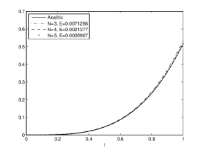
(a) ${{}_{0}I_{t}^{0.5}}(t^{3})$

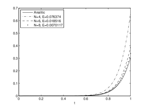
(b) ${{}_{0}I_{t}^{0.5}}(t^{10})$

Figure 1: Analytic versus numerical approximation for a fixed $n$.

Secondly, we apply our procedure to the transcendental functions $x_{3}(t)=e^{t}$ and $x_{4}(t)=\sin(t)$. Simple calculations give

$${{}_{0}I_{t}^{0.5}}x_{3}(t)=\sqrt{t}\sum_{k=0}^{\infty}\frac{t^{k}}{\Gamma(k+1.5)}\ \mbox{ and }\ {{}_{0}I_{t}^{0.5}}x_{4}(t)=\sqrt{t}\sum_{k=0}^{\infty}\frac{(-1)^{k}t^{2k+1}}{\Gamma(2k+2.5)}.$$

Figures 2(a) and 2(b) show the numerical results for each approximation, with $n=3$. We see that for a small value of $N$ one already obtains a good approximation for each function.

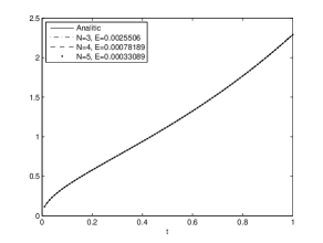
(a) ${{}_{0}I_{t}^{0.5}}(e^{t})$

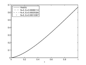
(b) ${{}_{0}I_{t}^{0.5}}(\sin(t))$

Figure 2: Analytic versus numerical approximation for a fixed $n$.

For analytical functions, we may apply the well-known formula (4). In Figure 3 we show the results of approximating with (4), $N=1,2,3$, for functions $x_{3}(t)$ and $x_{4}(t)$. We remark that, when we consider expansions up to the second derivative, i.e., the cases $n=3$ as in (5) and expansion (4) with $N=2$, we obtain a better accuracy using our approximation (5) even for a small value of $N$.

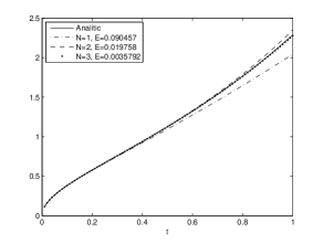
(a) ${{}_{0}I_{t}^{0.5}}(e^{t})$

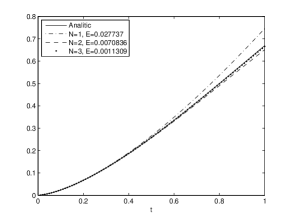
(b) ${{}_{0}I_{t}^{0.5}}(\sin(t))$

Figure 3: Numerical approximation using (4) of previous literature.

Another way to approximate fractional integrals is to fix $N$ and consider several sizes for the decomposition, i.e., letting $n$ to vary. Let us consider the two test functions $x_{1}(t)=t^{3}$ and $x_{2}(t)=t^{10}$, with $t\in[0,1]$ as before. In both cases we consider the first three approximations of the fractional integral, i.e., for $n=1,2,3$. For the first function we fix $N=3$, for the second one we choose $N=8$. Figures 4(a) and 4(b) show the numerical results. As expected, for a greater value of $n$ the error decreases.

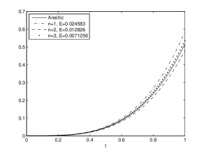
(a) ${{}_{0}I_{t}^{0.5}}(t^{3})$

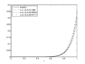
(b) ${{}_{0}I_{t}^{0.5}}(t^{10})$

Figure 4: Analytic versus numerical approximation for a fixed $N$.

We mentioned before that although the terms $A_{i}$ are all equal to zero, for $i\in\{0,\ldots,n-1\}$, we consider them in the decomposition formula. Indeed, after we truncate the sum, the error is lower. This is illustrated in Figures 5(a) and 5(b), where we study the approximations for ${{}_{0}I_{t}^{0.5}}x_{1}(t)$ and ${{}_{0}I_{t}^{0.5}}x_{2}(t)$ with $A_{i}\not=0$ and $A_{i}=0$.

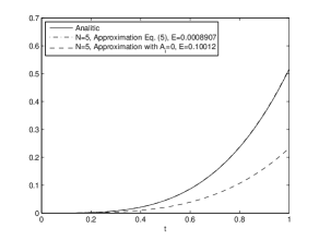
(a) ${{}_{0}I_{t}^{0.5}}(t^{3})$

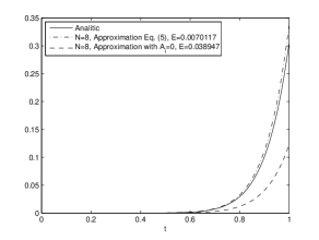
(b) ${{}_{0}I_{t}^{0.5}}(t^{10})$

Figure 5: Comparison of approximation (5) and approximation with $A_{i}=0$.

6 Applications

In this section we show how the proposed approximations can be applied into different subjects. For that, we consider a fractional integral equation (Example 6.1) and a fractional variational problem in which the Lagrangian depends on the left Riemann–Liouville fractional integral (Example 6.2). The main idea is to rewrite the initial problem by replacing the fractional integrals by an expansion of type (3) or (8), and thus getting a problem involving integer derivatives, which can be solved by standard techniques.

Example 6.1 (Fractional integral equation).

Consider the following fractional system:

$$\left\{\begin{array}[]{l}{{}_{0}I_{t}^{0.5}}x(t)=\frac{\Gamma(4.5)}{24}t^{4}\\ x(0)=0.\end{array}\right.$$ (16)

Since ${{}_{0}I_{t}^{0.5}}t^{3.5}=\frac{\Gamma(4.5)}{24}t^{\alpha}$, the function $t\mapsto t^{3.5}$ is a solution to problem (16).

To provide a numerical method to solve such type of systems, we replace the fractional integral by approximations (4) and (12), for a suitable order. We remark that the order of approximation, $N$ in (4) and $n$ in (12), are restricted by the number of given initial or boundary conditions. Since (16) has one initial condition, in order to solve it numerically, we will consider the expansion for the fractional integral up to the first derivative, i.e., $N=1$ in (4) and $n=2$ in (12). The order $N$ in (12) can be freely chosen.

Applying approximation (4), with $\alpha=0.5$, we transform (16) into the initial value problem

$$\left\{\begin{array}[]{l}1.1285t^{0.5}x(t)-0.3761t^{1.5}x^{\prime}(t)=\frac{\Gamma(4.5)}{24}t^{4},\\ x(0)=0,\end{array}\right.$$

which is a first order ODE. The solution is shown in Figure 6(a). It reveals that the approximation remains close to the exact solution for a short time and diverges drastically afterwards. Since we have no extra information, we cannot increase the order of approximation to proceed.

To use expansion (8), we rewrite the problem as a standard one, depending only on a derivative of first order. The approximated system that we must solve is

$$\left\{\begin{array}[]{l}A_{0}(0.5,N)t^{0.5}x(t)+A_{1}(0.5,N)t^{1.5}x^{\prime}(t)+\sum_{p=2}^{N}B(0.5,p)t^{1.5-p}V_{p}(t)=\frac{\Gamma(4.5)}{24}t^{4},\\ V_{p}^{\prime}(t)=(p-1)t^{p-2}x(t),\quad p=2,3,\ldots,N,\\ x(0)=0,\\ V_{p}(0)=0,\quad p=2,3,\ldots,N,\\ \end{array}\right.$$

where $A_{0},A_{1}$ are given as in (13) and $B$ is given by Theorem 3.3. Here, by increasing $N$, we get better approximations to the fractional integral and we expect more accurate solutions to the original problem (16). For $N=2$ and $N=3$ we transform the resulting system of ordinary differential equations to a second and a third order differential equation respectively. Finally, we solve them using the Maple built in function dsolve. For example, for $N=2$ the second order equation takes the form

$$\left\{\begin{array}[]{l}V_{2}^{\prime\prime}(t)=\frac{6}{t}V_{2}^{\prime}(t)+\frac{6}{t^{2}}V_{2}(t)-5.1542t^{2.5}\\ V(0)=0\\ V^{\prime}(0)=x(0)=0\end{array}\right.$$

and the solution is $x(t)=V_{2}^{\prime}(t)=1.34t^{3.5}$. In Figure 6(b) we compare the exact solution with numerical approximations for two values of $N$.

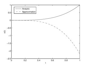
(a) Approximation by (4)

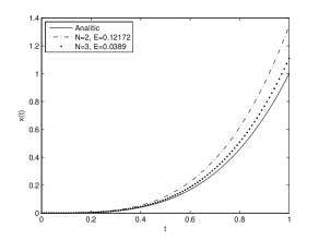
(b) Approximation by (12)

Figure 6: Analytic versus numerical solution to problem (16).

Example 6.2 (Fractional variational problem).

Let $\alpha\in(0,1)$. Consider the problem

$$\begin{gathered}J[x(\cdot)]=\int_{0}^{1}\left({{}_{0}I_{t}^{\alpha}}x(t)-t\right)^{2}dt\longrightarrow\min,\\ x(0)=0,\quad x(1)=\frac{\Gamma(\alpha+1.5)}{\Gamma(1.5)}.\end{gathered}$$ (17)

Problems of the calculus of variations of type (17), with a Lagrangian depending on fractional integrals, were first introduced in [3]. In this case the solution is rather obvious. Indeed, for

$$x(t)=\frac{\Gamma(1.5+\alpha)}{\Gamma(1.5)}\sqrt{t}$$ (18)

one has ${{}_{0}I_{t}^{\alpha}}x(t)=t$ and $J[x(\cdot)]=0$. Since functional $J$ is non-negative, (18) is the global minimizer of (17).

Using (12), we approximate problem (17) by

$$\begin{gathered}\tilde{J}[x(\cdot)]=\int_{0}^{1}\left[A_{0}(\alpha,N)t^{\alpha}x(t)+A_{1}(\alpha,N)t^{1+\alpha}x^{\prime}(t)+\sum_{p=2}^{N}B(\alpha,p)t^{1+\alpha-p}V_{p}(t)-t\right]dt\longrightarrow\min,\\ V_{p}^{\prime}(t)=(p-1)t^{p-2}x(t),\quad p=2,3,\ldots,N,\\ V_{p}(0)=0,\quad p=2,3,\ldots,N,\\ x(0)=0,\quad x(1)=\frac{\Gamma(\alpha+1.5)}{\Gamma(1.5)}.\end{gathered}$$ (19)

This is a classical variational problem, constrained by a set of boundary conditions and ordinary differential equations. One way to solve such a problem is to reformulate it as an optimal control problem [15]. Let us introduce the control variable

$$u(t)=A_{0}(\alpha,N)t^{\alpha}x(t)+A_{1}(\alpha,N)t^{1+\alpha}x^{\prime}(t)+\sum_{p=2}^{N}B(\alpha,p)t^{1+\alpha-p}V_{p}(t).$$

Then (19) becomes the classical optimal control problem

$$\begin{gathered}\tilde{J}[x(\cdot)]=\int_{0}^{1}\left[u(t)-t\right]dt\longrightarrow\min,\\ x^{\prime}(t)=-A_{0}A_{1}^{-1}t^{-1}x(t)-\sum_{p=2}^{N}A_{1}^{-1}B_{p}t^{-p}V_{p}(t)+A_{1}^{-1}t^{-1-\alpha}u(t),\\ V_{p}^{\prime}(t)=(p-1)t^{p-2}x(t),\quad p=2,3,\ldots,N,\\ V_{p}(0)=0,\quad p=2,3,\ldots,N,\\ x(0)=0,\quad x(1)=\frac{\Gamma(\alpha+1.5)}{\Gamma(1.5)},\end{gathered}$$

where $A_{i}=A_{i}(\alpha,N)$ and $B_{p}=B(\alpha,p)$. For $\alpha=0.5$ and $N=2$, application of the Hamiltonian system with multipliers $\lambda_{1}(t)$ and $\lambda_{2}(t)$ [15], gives the two point boundary value problem

$$\left\{\begin{array}[]{rl}x^{\prime}(t)&=-A_{0}A_{1}^{-1}t^{-1}x(t)-A_{1}^{-1}B_{2}t^{-2}V_{2}(t)t^{1-\alpha}-\frac{1}{2}A_{1}^{-2}t^{-2-2\alpha}\lambda_{1}(t)+A_{1}^{-1}t^{-\alpha},\\ V_{2}^{\prime}(t)&=x(t),\\ \lambda_{1}^{\prime}(t)&=A_{0}A_{1}^{-1}t^{-1}\lambda_{1}(t)-\lambda_{2}(t),\\ \lambda_{2}^{\prime}(t)&=A_{1}^{-1}B_{2}t^{-2}\lambda_{1}(t),\\ \end{array}\right.$$ (20)

with boundary conditions

$$\left\{\begin{array}[]{l}x(0)=0,\\ V_{2}(0)=0,\end{array}\right.\qquad\left\{\begin{array}[]{l}x(1)=1,\\ \lambda_{2}(1)=0.\end{array}\right.$$

In practice the value of $n$ is chosen taking into account the number of boundary conditions. For problem (17), to avoid lack of boundary conditions, we take $n=2$. On the other hand, the value of $N$ is only restricted by the computational power and the efficiency of the numerical method chosen to solve the approximated problem. Figure 7 shows the solution to system (20) together with the exact solution to problem (17) and corresponding values of $J$.

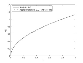
Figure 7: Analytic versus numerical solution to fractional variational problem (17).

References

- [1] R. Almeida, A. B. Malinowska and D. F. M. Torres, A fractional calculus of variations for multiple integrals with application to vibrating string, J. Math. Phys. 51 (2010), no. 3, 033503, 12 pp. arXiv:1001.2722
- [2] R. Almeida, S. Pooseh and D. F. M. Torres, Fractional variational problems depending on indefinite integrals, Nonlinear Anal. 75 (2012), no. 3, 1009–1025. arXiv:1102.3360
- [3] R. Almeida and D. F. M. Torres, Calculus of variations with fractional derivatives and fractional integrals, Appl. Math. Lett. 22 (2009), no. 12, 1816–1820. arXiv:0907.1024
- [4] R. Almeida and D. F. M. Torres, Leitmann’s direct method for fractional optimization problems, Appl. Math. Comput. 217 (2010), no 3, 956–962. arXiv:1003.3088
- [5] G. E. Andrews, R. Askey and R. Roy, Special functions, Encyclopedia of Mathematics and its Applications, 71, Cambridge Univ. Press, Cambridge, 1999.
- [6] T. M. Atanackovic and B. Stankovic, On a numerical scheme for solving differential equations of fractional order, Mech. Res. Comm. 35 (2008), no. 7, 429–438.
- [7] R. Beals and R. Wong, Special functions, Cambridge Studies in Advanced Mathematics, 126, Cambridge Univ. Press, Cambridge, 2010.
- [8] G. S. F. Frederico and D. F. M. Torres, Fractional conservation laws in optimal control theory, Nonlinear Dynam. 53 (2008), no. 3, 215–222. arXiv:0711.0609
- [9] A. A. Kilbas, H. M. Srivastava and J. J. Trujillo, Theory and applications of fractional differential equations, North-Holland Mathematics Studies, 204, Elsevier, Amsterdam, 2006.
- [10] C. Li A. Chen and J. Ye, Numerical approaches to fractional calculus and fractional ordinary differential equation, J. Comput. Phys. 230 (2011), no. 9, 3352–3368.
- [11] J. T. Machado, V. Kiryakova and F. Mainardi, Recent history of fractional calculus, Commun. Nonlinear Sci. Numer. Simul. 16 (2011), no. 3, 1140–1153.
- [12] A. B. Malinowska and D. F. M. Torres, Generalized natural boundary conditions for fractional variational problems in terms of the Caputo derivative, Comput. Math. Appl. 59 (2010), no. 9, 3110–3116. arXiv:1002.3790
- [13] K. S. Miller and B. Ross, An introduction to the fractional calculus and fractional differential equations, A Wiley-Interscience Publication, Wiley, New York, 1993.
- [14] D. Mozyrska and D. F. M. Torres, Modified optimal energy and initial memory of fractional continuous-time linear systems, Signal Process. 91 (2011), no. 3, 379–385. arXiv:1007.3946
- [15] L. S. Pontryagin, V. G. Boltyanskii, R. V. Gamkrelidze and E. F. Mishchenko, The mathematical theory of optimal processes, Translated from the Russian by K. N. Trirogoff; edited by L. W. Neustadt Interscience Publishers John Wiley & Sons, Inc. New York, 1962.
- [16] S. G. Samko, A. A. Kilbas and O. I. Marichev, Fractional integrals and derivatives, translated from the 1987 Russian original, Gordon and Breach, Yverdon, 1993.
- [17] Q. Yang, F. Liu and I. Turner, Numerical methods for fractional partial differential equations with Riesz space fractional derivatives, Appl. Math. Model. 34 (2010), no. 1, 200–218.