Analytical and Monte Carlo results for the surface-brightness diameter relationship in supernova remnants

Abstract

The surface brightness diameter relationship for supernovae remnants (SNRs) is explained by adopting a model of direct conversion of the flux of kinetic energy into synchrotron luminosity. Two laws of motion are adopted, a power law model for the radius-time relationship, and a model which uses the thin layer approximation. The fluctuations on the log-log surface diameter relationship are modeled by a Monte Carlo simulation. In this model a new probability density function for the density as function of the galactic height is introduced.

1 Introduction

The correlation between radio surface brightness, $\Sigma_{1GHz}$, and diameter $D$ in pc in supernova remnants is parametrized as

$$\Sigma_{1GHz}=C_{\Sigma}(D)^{-\beta_{\Sigma}}\quad\frac{W}{m^{2}\,Hz\,sr}\quad,$$ (1)

where ${\beta_{\Sigma}}$ and $C_{\Sigma}$ are are found through the radio observations (Shklovskii, 1960; Urošević et al., 2005). This is an observational relationship which has been explained by early theoretical models (Lequeux, 1962; Poveda & Woltjer, 1968; Kesteven, 1968; Clark & Caswell, 1976; Milne, 1979). A theoretical interpretation of the $\Sigma-D~{}$relationship has been introduced by Duric & Seaquist (1986) by incorporating the Sedov blast wave solution for supernovae remnant (SNR) expansion, the generation and evolution of the magnetic field as outlined by Gull (1973), and the acceleration of relativistic electrons by shocks, as formulated by Bell (1978a, b). The time-dependent, nonlinear kinetic theory for cosmic ray (CR) production was adopted by Berezhko & Völk (2004) in order to derive a theoretically predicted brightness-diameter relation in the radio range for the Sedov phase. Recently Bandiera & Petruk (2010) found that SNRs cease to emit effectively in radio at a stage near the end of their Sedov evolution, and that models of synchrotron emission with constant efficiencies in particle acceleration and magnetic field amplification do not provide a close match to the data. These previous models leave a series of questions unanswered or merely partially answered:

• Is it possible to deduce a theoretical $\Sigma-D~{}$relationship on the basis of power law expansion for SNR?

• Is it possible to deduce a classical equation of expansion for the SNR with two adjustable parameters that can be found from a numerical analysis of the radius–time relationship?

• Is the theoretical $\Sigma-D~{}$relationship sensitive to the density of the interstellar medium, which decreases as a function of height above the galactic plane?

In order to answer these questions, we develop a theoretical derivation of the $\Sigma-D~{}$relationship by modeling the expansion of a synchrotron emitting shell. In Section 2, we show that it is reasonable to fit a power-law expansion relationship to a known young supernova remnant, SN 1987J in M81, for which the growth of the shell like structure is available over a period of 10 years. In Section 3, we discuss a modification of the power-law expansion model for the effects of the standard gradient in density in the interstellar medium. In Section 4, we complete our derivation of the $\Sigma-D~{}$relationship by adopting a direct conversion of the flux of kinetic energy into radiation calibrated on the observational data (Section 5). In Section 6, we address the observed fluctuations in the $\Sigma-D~{}$relationship by utilizing a new probability density function (PDF) for the contrast of in situ densities of SNRs. This new PDF is derived from the standard number distribution of SNRs with the galactic height.

2 The Power Law Model of Expansion

A standard point of view assumes that the SNR expands at a constant velocity until the surrounding mass is of the order of the solar mass. This time scale can be modeled by

$$t_{M}=186.45\,{\frac{\sqrt[3]{{\it M_{\sun}}}}{\sqrt[3]{{\it n_{0}}}{\it v_{10000}}}}\quad yr\quad,$$ (2)

where $M_{\sun}$ is the number of solar masses in the volume occupied by the SNR, $n_{0}$, the number density expressed in particles $\mathrm{cm}^{-3}$, and $v_{10000}$ the initial velocity expressed in units of $10000\,km/s$ , see McCray (1987). To model the time-dependent expansion of SNRs, we use

$$R(t)=Ct^{\alpha}\quad,$$ (3)

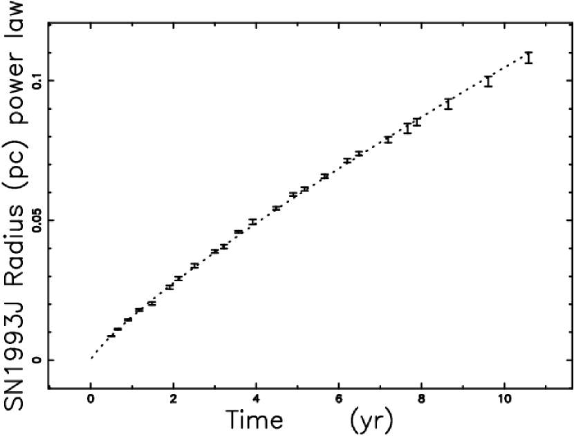
Figure 1: Theoretical radius as given by the power law model with data as in Table 1 (full line), and astronomical data of SN 1993J with vertical error bars.

where the two parameters $C$ and $\alpha$ can be found from the observations. Ten years of observations of SN 1993J (Marcaide et al., 2009) allow us to fit these two parameters which are reported in Table 1 and in Figure 1. The quality of the fit is measured by the merit function

$$\chi^{2}=\sum_{j}\frac{(R_{th}-R_{obs})^{2}}{\sigma_{obs}^{2}}\quad,$$ (4)

where $R_{th}$, $R_{obs}$ and $\sigma_{obs}$ are the theoretical radius, the observed radius and the observed uncertainty respectively. This observed relationship allows us to express the radius, as a function of time, by

$$R(t)=0.0155\,{t}^{0.828}\quad pc\quad,$$ (5)

where the time $t$ is expressed in $yr$. The velocity in this model is

$$V(t)=12587.67\,{t}^{-0.171}\frac{km}{s}\quad.$$ (6)

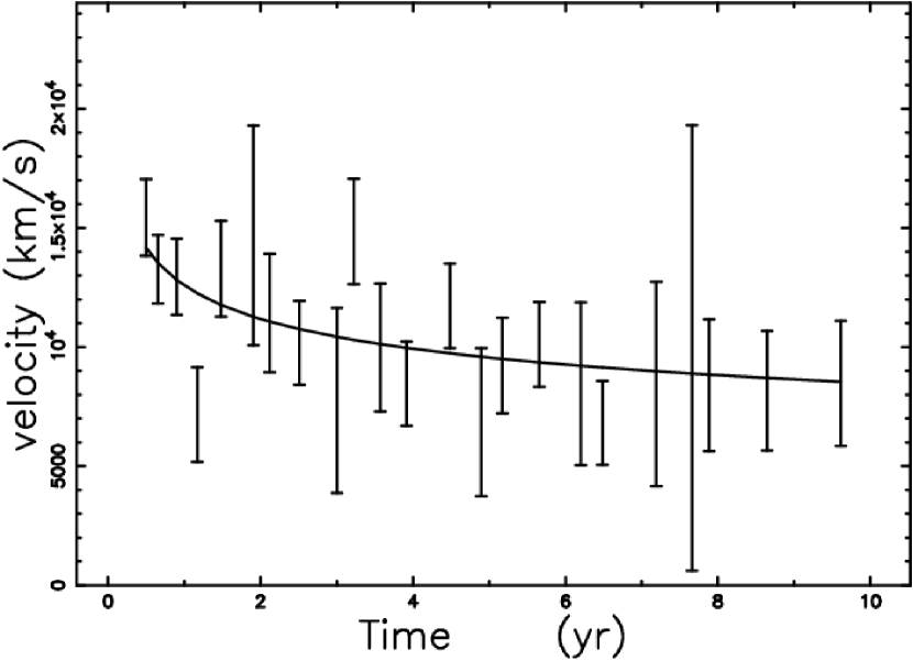
Figure 2: Theoretical velocity as given by Eq. (6) (full line) and instantaneous velocity of SN 1993J with uncertainty.

Figure 2 displays the observed instantaneous velocity as deduced from the finite difference method and the best fit according to Eq. (6). Another interesting SNR is SN 1006  which started to be visible in 1006 AD and has an actual radius of $15^{\prime}$ according to Green (2009). The radius in pc is a function of the the adopted distance; as an example, Katsuda et al. (2010) quotes a distance of 2.2 kpc and Winkler et al. (2003) 2.18 kpc. Here we adopt a distance of 2.2 kpc and consequently the observed radius, $R_{obs}$, is

$$R=9.59D_{22}\,pc\quad,$$ (7)

where the $D_{22}$ is the distance expressed in units of 2.2 kpc. The proper motion of the remnant’s edge is a weak function of the azimuth angle and the average value is

$$\overline{P_{obs}}=0.5\,arcsec/yr\quad.$$ (8)

The average velocity of the expansion is

$$V_{obs}=5441\,D_{22}\frac{km}{s}\quad.$$ (9)

Eq. (3) and the connected velocity can be solved for the two unknown variables $\alpha$ and $C$

$$\alpha=0.000001022\,{\frac{{\it V_{obs}}\,t}{{\it R_{obs}}}}$$

$$C=\frac{\it R_{obs}}{{t}^{0.000001022\,{\frac{{\it V_{obs}}\,t}{{\it R_{obs}}}}}}$$ (10)

where $V_{obs}$ is expressed in $\frac{km}{s}$ , $R_{obs}$ in pc and $t$ in yr. Table 2 reports the numerical results.

3 Momentum conservation and galactic height

The presence of a slow wind from the SN progenitor makes it reasonable for us to assume that the SNR evolves in a previously ejected medium phase in which density is considerably higher than the interstellar medium (ISM). The assumption used here is that the density of the ISM around the SNR has the following two piecewise dependencies

$$\rho(R)=\left\{\begin{array}[]{ll}\rho_{0}&\mbox{if $R\leq R_{0}$ }\\ f\,\rho_{0}(\frac{R_{0}}{R})^{d}&\mbox{if $R>R_{0}$ ~{}.}\end{array}\right.$$ (11)

where $f$ is a parameter that models the jump in density , $0<f\leq 1$, and is connected with the vertical profile in density as a function of the galactic height. In this framework, the density decreases as an inverse power law with an exponent $d$ that can be fixed from the observed temporal evolution of the radius, with $d=0$ meaning constant density; further on the parameter $f$ regulates the density at $R=R_{0}$. The swept mass in the interval $0\leq r\leq R_{0}$ is

$$M_{0}=\frac{4}{3}\,\rho_{{0}}\pi\,{R_{{0}}}^{3}\quad.$$ (12)

The swept mass in the interval $0\leq r\leq R$ with $r\geq R_{0}$ is

$$M=-4\,f\,{r}^{3}\rho_{{0}}\pi\,\left({\frac{R_{{0}}}{r}}\right)^{d}\left(d-3\right)^{-1}$$

$$+4\,f\,{\frac{\rho_{{0}}\pi\,{R_{{0}}}^{3}}{d-3}}+\frac{4}{3}\,\rho_{{0}}\pi\,{R_{{0}}}^{3}\quad.$$ (13)

Momentum conservation requires that

$$Mv=M_{0}v_{0}\quad,$$ (14)

where $v$ is the velocity at $t$ and $v_{0}$ is the velocity at $t=t_{0}$. The velocity as a function of the radius is

$$v=\frac{v_{{0}}{r_{{0}}}^{3}\left(3-d\right)}{3\,{r_{{0}}}^{d}{R}^{3-d}f+{r_{{0}}}^{3}\left(-d+3-3\,f\right)}\quad.$$ (15)

In this first order differential equation in R, the variables can be separated and an integration term by term yields the following nonlinear equation

$${\mathcal{F}}_{NL}=$$

$$\left(12\,{R_{{0}}}^{3}f-3\,{R_{{0}}}^{3}fd+7\,{R_{{0}}}^{3}d-{R_{{0}}}^{3}{d}^{2}-12\,{R_{{0}}}^{3}\right)R$$

$$-3\,{R_{{0}}}^{d}f{R}^{4-d}+7\,{R_{{0}}}^{3}v_{{0}}dt_{{0}}+{R_{{0}}}^{3}v_{{0}}{d}^{2}t$$

$$-{R_{{0}}}^{3}v_{{0}}{d}^{2}t_{{0}}+{R_{{0}}}^{4}{d}^{2}+12\,{R_{{0}}}^{4}-9\,{R_{{0}}}^{4}f-7\,{R_{{0}}}^{4}d-7\,{R_{{0}}}^{3}v_{{0}}dt$$

$$-12\,{R_{{0}}}^{3}v_{{0}}t_{{0}}+3\,{R_{{0}}}^{4}fd+12\,{R_{{0}}}^{3}v_{{0}}t\quad.$$ (16)

An approximate solution of ${\mathcal{F}}_{NL}(r)$ can be obtained assuming that
$3R_{0}^{d}R^{4-d}f$ $\gg$ ${R_{{0}}}^{3}\left(4-d\right)\left(d-3+3\,f\right)R$

$$R(t)=$$

$$({R_{{0}}}^{4-d}-\frac{1}{3f}(d-3+3f){R_{{0}}}^{4-d}(4-d)$$

$$+\frac{1}{3f}(4-d)v_{{0}}{R_{{0}}}^{3-d}(3-d)(t-t_{{0}}))^{\frac{1}{4-d}}\quad.$$ (17)

The physical units have not been specified, $pc$ for length and $yr$ for time are perhaps an acceptable astrophysical choice. With these units, the initial velocity $v_{{0}}$ is expressed in $\frac{pc}{yr}$ and should be converted into $\frac{km}{s}$; this means that $v_{{0}}=1.02\,10^{-6}v_{{1}}$ where $v_{{1}}$ is the initial velocity expressed in $\frac{km}{s}$.

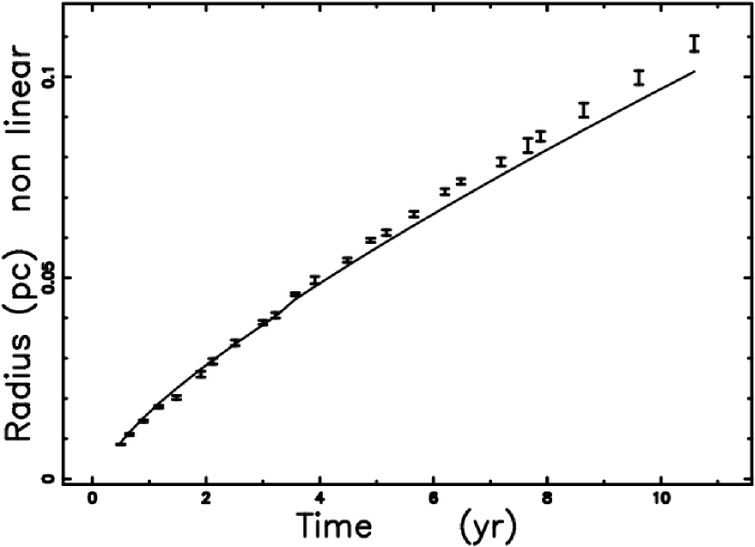
Figure 3: Theoretical radius as obtained by the solution of the nonlinear Eq. (16) (full line), data as in Table 1 and $f$=1. The astronomical data of SN 1993J are represented with vertical error bars.

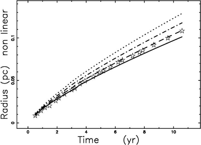
Figure 4: The same as Figure 3 but $f$ is variable; $f=1$ (full line), $f=0.9$ (dashed) , $f=0.8$ (dot-dash-dot-dash) $f=0.7$ (dotted) and experimental point represented by empty stars.

A one-dimensional solution of Eq. (16) can be found with the FORTRAN subroutine ZRIDDR (Press et al., 1992). A plot of this radial solution, using a parameter value of f = 1, is shown in Figure (3). Plots of other solutions with different value of f can be found in Figure (4).

4 $\Sigma-D~{}$in the power law model

In this section, we review the time scale of synchrotron losses, the time scale of acceleration and the inequality which allows us to use the in situ acceleration of electrons. The relation between the radio surface brightness and diameter of SNRs is deduced assuming a direct proportionality between the radio-luminosity and the flux of kinetic energy.

4.1 The synchrotron emission

An electron which loses its energy due to synchrotron radiation has a lifetime of

$$\tau_{r}\approx\frac{E}{P_{r}}\approx 500E^{-1}H^{-2}sec\quad,$$ (18)

where $E$ is the energy in ergs, $H$ the magnetic field in Gauss, and $P_{r}$ is the total radiated power (Lang, 1999, Eq. 1.157). The energy is connected to the critical frequency (Lang, 1999, Eq. 1.154), as

$$\nu_{c}=6.266\times 10^{18}HE^{2}~{}Hz\quad.$$ (19)

The lifetime for synchrotron losses is

$$\tau_{syn}=39660\,{\frac{1}{H\sqrt{H\nu}}}\,yr\quad.$$ (20)

Following (Fermi, 1949, 1954), the gain in energy in a continuous form for a particle which spirals around a line of force is proportional to its energy, $E$,

$$\frac{dE}{dt}=\frac{E}{\tau_{II}}\quad,$$ (21)

where $\tau_{II}$ is the typical time-scale,

$$\frac{1}{\tau_{II}}=\frac{4}{3}(\frac{u^{2}}{c^{2}})(\frac{c}{L})\quad,$$ (22)

where $u$ is the velocity of the accelerating cloud, $c$ is the velocity of the light and $L$ is the mean free path between clouds (Lang, 1999, Eq. 4.439). The mean free path between the accelerating clouds in the Fermi II mechanism can be found from the following inequality in time :

$$\tau_{II}<\tau_{sync}\quad,$$ (23)

which corresponds to the following inequality for the mean free path between scatterers

$$L<\frac{1.72\,10^{5}\,{u}^{2}}{H\sqrt{H\nu}{c}^{2}}\,pc\quad.$$ (24)

The mean free path length for SN 1993J at $\nu=1GHz$ gives

$$L<1.83\,10^{-5}{t}^{-0.34}\,pc$$ (25)

where the velocity is given by Eq.(6) and $H=65.1\,G$ (Martí-Vidal et al., 2011). When this inequality is verified the direct conversion of the flux of kinetic energy into radiation can be adopted. Recall that the Fermi II mechanism produces an inverse power law spectrum in the energy of the type $N(E)\propto E^{-\gamma}$ or an inverse power law in the observed frequencies $N(\nu)\propto\nu^{-\alpha}$ with $\alpha=\frac{\gamma-1}{2}$ (Lang, 1999; Zaninetti, 2011).

4.2 The dimensional approach

The source of synchrotron luminosity is here assumed to be the flux of kinetic energy

$$L_{m}=\frac{1}{2}\rho AV^{3}\quad,$$ (26)

where A is the emitting surface area (de Young, 2002, Eq. A28). Assuming the surface area is like that of a sphere, the luminosity is

$$L_{m}=\frac{1}{2}\rho 4\pi R^{2}V^{3}\quad,$$ (27)

where $R$ is the instantaneous radius of the SNR and $\rho$ is the density in the advancing layer in which the synchrotron emission takes place. Assuming the density of the advancing layer scales as $R^{-d}$, which means that

$$L_{m}\propto R^{2-d}V^{3}\quad.$$ (28)

The time dependence is eliminated by utilizing Eq. (3)

$$L_{m}=L_{0}(\frac{R}{R_{0}})^{-{\frac{d\alpha-5\,\alpha+3}{\alpha}}}\quad,$$ (29)

where $L$ is the luminosity at $R=R_{0}$ or

$$L_{m}=L_{0}(\frac{D}{D_{0}})^{-{\frac{d\alpha-5\,\alpha+3}{\alpha}}}\quad,$$ (30)

where $D$ is the actual diameter and $D_{0}=2R_{0}$. On assuming that the observed luminosity ,$L_{\nu}$, in a given band denoted by the frequency $\nu$ is proportional to the mechanical luminosity we obtain

$$L_{\nu}=L_{0,\nu}(\frac{D}{D_{0}})^{-{\frac{d\alpha-5\,\alpha+3}{\alpha}}}\quad Jy\,kpc^{2}\quad,$$ (31)

where $L_{0,\nu}$ is the observed radio luminosity in a given band. The observations are generally represented in the form

$$L=C_{L}D^{-\beta_{L}}\quad,$$ (32)

where $L$ and $C_{L}$ are parameters deduced from the radio observations (Guseinov et al., 2003; Urošević et al., 2005). Given the two observational parameters $\alpha$ and $\beta_{L}$ we can derive

$$d={\frac{\beta_{L}\,\alpha+5\,\alpha-3}{\alpha}}\quad.$$ (33)

The radio surface brightness of a remnant is defined as

$$\Sigma=\frac{S_{1GHz}}{\theta^{2}}\quad,$$ (34)

where $S_{1GHz}$ is the detected flux of a remnant at $1GHz$ and $\theta$ the observed angle. Due to the fact that $\theta\propto D^{2}$ we have

$$\Sigma_{1GHz}=\Sigma_{0,1GHz}(\frac{D}{D_{0}})^{-{\frac{d\alpha-3\,\alpha+3}{\alpha}}}\quad\frac{W}{m^{2}\,Hz\,sr}\quad,$$ (35)

where $\Sigma_{0,{1GHz}}$ is the surface brightness at $D=D_{0}$ . According to the basic observational relationship (1)

$$d={\frac{{\it\beta_{\Sigma}}\,\alpha+3\,\alpha-3}{\alpha}}\quad.$$ (36)

5 Observations in the power law model

Supernova remnants in our galaxy have two luminosity-diameter relationships (Guseinov et al., 2003): the first one for SNRs which have L $>$ 5300 Jy kpc², D $<$ 36.5 pc and the second one for SNRs having L $\leq$ 5300 Jy kpc², D $\geq$ 36.5 pc,

$$L=2.45\,10^{4}D^{-0.43}\hskip 8.5359ptJy\hskip 2.84544ptkpc^{2}\quad D<36.5pc\quad,$$ (37)

and

$$L=5.38\,10^{9}D^{-3.84}\hskip 8.5359ptJy\hskip 2.84544ptkpc^{2}\quad D\geq 36.5pc\quad.$$ (38)

The $\Sigma-D~{}$relationship in a similar way is

$$\Sigma=2.7^{+2.1}_{-1.4}\,10^{-17}D^{{-2.47}^{+0.20}_{-0.16}}\hskip 8.5359ptWm^{-2}Hz^{-1}ster^{-1}\quad D<36.5pc\quad,$$ (39)

and

$$\Sigma=8.4^{+19.5}_{-6.3}\,10^{-12}D^{{-5.99}^{+0.38}_{-0.33}}\hskip 8.5359ptWm^{-2}Hz^{-1}ster^{-1}\quad D\geq 36.5pc\quad.$$ (40)

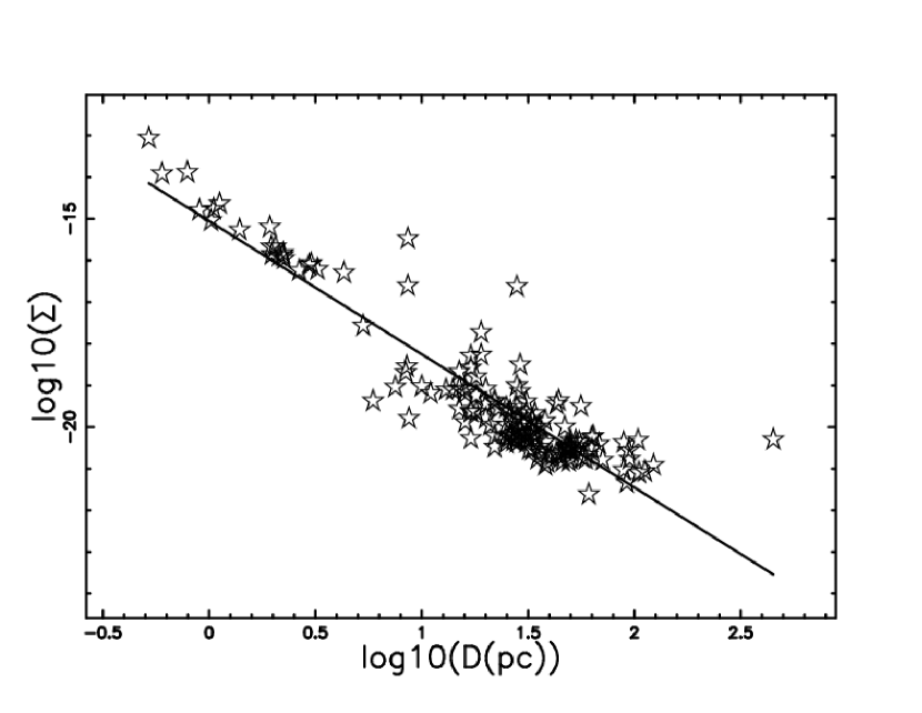
Figure 5: The LOG-LOG $\Sigma-D~{}$diagram at a frequency of 1 GHz for all the extragalactic SNRs as given by Urošević et al. (2005).

The observations of the surface brightness of SNRs in other galaxies has been analyzed by Urošević et al. (2005) with data available at Centre de Données astronomiques de Strasbourg (CDS). Figure 5 reports the observational data as well the fitting curve of all the radio SNRs in external galaxies. The results of our numerical analysis for extragalactic SNRs gives

$$\Sigma=(8.8\pm 3.27\,10^{-16}D^{-3.1\pm 0.11}\hskip 8.5359ptWm^{-2}Hz^{-1}ster^{-1}\quad D<450pc\quad,$$ (41)

which agrees with the results of Urošević et al. (2005). The values of $d$ from the
$\Sigma-D~{}$relationship are reported in Table 3.

6 A Monte Carlo model for $\Sigma-D~{}$

The significant fluctuations observed in the $\Sigma-D~{}$relationship can be explained by correlating the well known probability to have a SNR at the galactic height $z$ with the density. This conversion can be done using the nonlinear relationship between $z$ and density as given by the self-gravitating disk.

The radius function we derived in Section 3 (Eq. 17) from momentum conservation allows us to deduce an analytical expression for the $\Sigma-D~{}$relationship:

$$\Sigma_{1GHz}=\Sigma_{0,1GHz}(\frac{1}{f^{3}})(\frac{D}{D_{0}})^{-{\frac{d\alpha-3\,\alpha+3}{\alpha}}}\quad\frac{W}{m^{2}\,Hz\,sr}\quad.$$ (42)

The $\Sigma-D~{}$relationship now has an inverse cubic dependence for the contrast parameter $f$.

6.1 The profile of the ISM

The vertical number density distribution of galactic H I has the following three component behavior as a function of the galactic height z , the distance from the galactic plane in pc :

$$n(z)=n_{1}e^{-z^{2}/{H_{1}}^{2}}+n_{2}e^{-z^{2}/{H_{2}}^{2}}+n_{3}e^{-|z|/{H_{3}}}\,.$$ (43)

We set the densities in Eq. (43) to $n_{1}=0.395$ particles cm^-3, $n_{2}=0.107$ particles cm^-3, $n_{3}=0.064$ particles cm^-3, and the scale heights to $H_{1}=127$ pc, $H_{2}=318$ pc, and $H_{3}=403$ (Lockman, 1984; Dickey & Lockman, 1990; Bisnovatyi-Kogan & Silich, 1995). This distribution of galactic H I is valid in the range 0.4 $\leq$ $R$ $\leq$ $R_{0}$, where $R_{0}$ = 8.5 kpc and $R$ is the distance from the galaxy center. The previous empirical relationship can be modelled by a theoretical one. The density profile of a thin self-gravitating disk of gas which is characterized by a Maxwellian distribution in velocity and distribution which varies only in the z-direction has the following number density distribution

$$n(z)=n_{0}sech^{2}(\frac{z}{2*z_{0}})\quad,$$ (44)

where $n_{0}$ is the density at $z=0$ and $z_{0}$ is a scaling parameter (Bertin, 2000; Padmanabhan, 2002). Figure (6) displays a comparison between the empirical function sum of three exponential disks and the theoretical function as given by the Eq. (44). The previous equation can be expressed with our contrast parameter $f$

$$f=sech^{2}(\frac{z}{2*z_{0}})\quad,$$ (45)

and the inversion gives $z$ as function of $f$

$$z=2\,{\it arcsech}\left(\sqrt{f}\right)z_{{0}}\quad.$$ (46)

6.2 The distribution of SNRs

The probability density function (PDF) ,$p(z)$, to have a SNR as function of the galactic height $z$ is characterized by an exponential PDF

$$p(z)=\frac{1}{b}\exp{-\frac{z}{b}}\quad,$$ (47)

with $b=83$ pc (Xu et al., 2005). The average value $\overline{z}$ for SNRs is

$$\overline{z}=b=83pc\quad.$$ (48)

We briefly review how a PDF $p(z)$ changes to $g(f)$ when a new variable $f(z)$ is introduced. The rule for transforming a PDF is

$$g(f)=\frac{p(f(z))}{|\frac{d(g(f))}{dz}|}\quad.$$ (49)

Once the previous rule is implemented we obtain

$$g(f)=\frac{{{\rm e}^{-2\,{\frac{{\it arcsech}\left(\sqrt{f}\right){\it z_{0}}}{b}}}}{\it z_{0}}}{b{f}^{3/2}\sqrt{{\frac{1}{\sqrt{f}}}-1}\sqrt{{\frac{1}{\sqrt{f}}}+1}}\quad.$$ (50)

The average value of $f$ when $b=83\,pc$ and $z_{0}$=90 is $\overline{f}=0.7927$.

6.3 Monte Carlo Simulation

We are ready to build a a Monte Carlo model for the $\Sigma-D$ distribution of SNRs for SNRs characterized by the following constraints

• The lifetime of a SNR is generated between 0 and $t_{max}$.

• The time is converted in diameter , $D=R*2$ , adopting Eq. (5).

• A value of $f$ is randomly generated according to the PDF, Eq. (50).

• In the previous points we have generated one $D$ and one $f$, as a consequence a value of $\Sigma_{1GHz}$ as given by Eq. (42) can be generated.

The results of this simulation are displayed in Figure 7 for the Galactic distribution, and in Figure 8 for the extragalactic distribution. In this Section we derived the profile of the density in our galaxy as function of the galactic height $z$ in the framework of the self-gravitating disk. This new relationship allows us to find a new PDF that characterizes the effect of SNRs expanding into a medium of varying density. The great fluctuations present in the galactic $\Sigma-D~{}$relationship are therefore explained by the SNR evolution in a medium with a lower density.

7 Conclusions

The relation between radio surface brightness and diameter of galactic and extragalactic SNRs presents a linear relationship in the Log( $\Sigma$)-D plane. Superposed on this observed linear behavior there is a fluctuation which is due to the variable density with the galactic height of the ISM. The major results of this paper are summarized as follows.

• The power law model for the expansion of a SNR coupled with a decreasing density medium allows to build a simple expression for the luminosity as well the radio surface brightness, see Eqs. (35) and (29).

• A more sophisticated approach to the law of motion as given by the momentum conservation in a medium with variable density allows to obtain the same result , see Eq. (42), once an asymptotic behavior for the law of motion is given, see Eq. (17). In this model is possible to introduce a contrast parameter $f$ which allows to state that both the radius and the velocity increase as $\frac{1}{f}$ and the surface brightness as $\frac{1}{f^{3}}$.

• The value of $f$ for each SNR is given by a new PDF (Eq. 50) which is derived from the observed PDF for SNR as function of the galactic height , see Eq. (47) and from a physical profile of density of the ISM as given by Eq. (44).

• A Monte Carlo simulation of the radio surface brightness explains the fluctuations visible in the $\Sigma-D~{}$relationship as a probabilistic effect to have a SNR with a given galactic height or $f$.

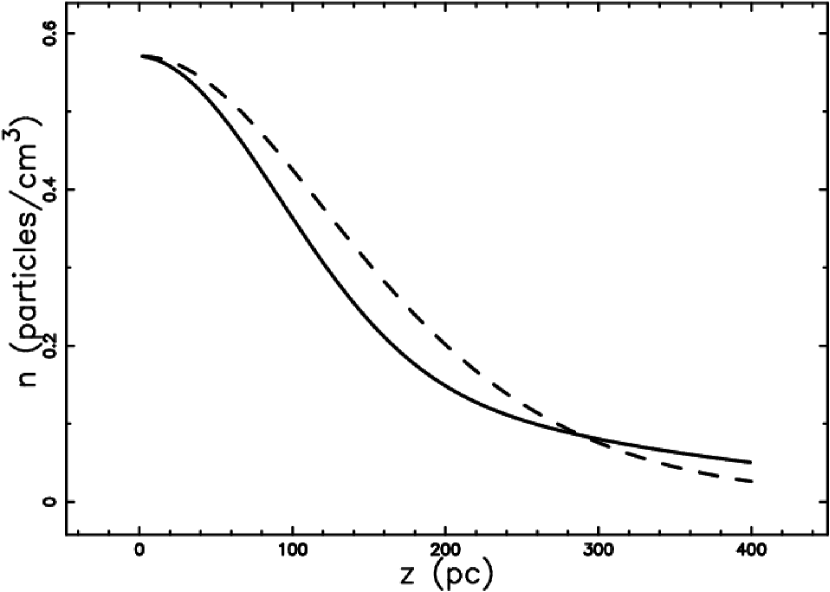
Figure 6: Profiles of density versus scale height $z$: the self-gravitating disk as given by Eq. (44) when $z_{0}=90~{}pc$ (dashed) and the three-component exponential distribution as given by Eq. (43) (full line).

Figure 7: A Monte Carlo LOG-LOG $\Sigma-D~{}$diagram at a frequency of 1 GHz which simulates the Galactic SNRs for $D<36.5pc$. The parameters are $t_{max}=5055\,yr$ , $\alpha$ = 0.82 , $b$ = 83 $pc$ and $z_{0}$ = 90  $pc$. The Monte Carlo simulation gives $C_{\Sigma}$ = $2.7110^{-17}$ and $\beta_{\Sigma}$=2.45.

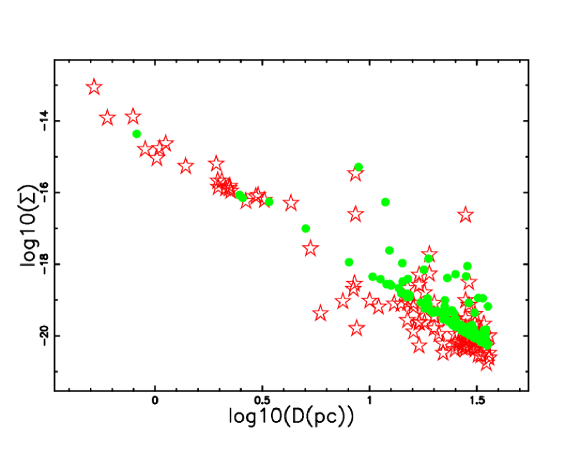
Figure 8: A Monte Carlo LOG-LOG $\Sigma-D~{}$diagram at a frequency of 1 GHz (green circles) and extragalactic SNRs as given by Urošević et al. (2005) for $D<36.5pc$ (empty red stars). The parameters are $t_{max}=2960yr$ , $C=0.17$ , $\alpha$ = 0.57 , $b$ = 83 $\,pc$ and $z_{0}$ = 60 $\,pc$. The Monte Carlo simulation gives $C_{\Sigma}$ = $8.8410^{-16}$ and $\beta_{\Sigma}$=3.65.

Table 1: Numerical values of the parameters of the fits for SN 1993J and $\chi^{2}$. $N$ represents the number of free parameters.

N values $$\chi^{2}$$

power law

2 = 0.82 0.0048 6364

C = (0.015 0.00011)

nonlinear radius

4 d=2.93; = 0.019 pc; 276

=0.249 yr; =100 000

Table 2: Numerical values of the parameters of the fits for SN 1006  as given by Eq. (10) for $R_{obs}$ = 9.59 pc , $V_{obs}$ =5441 $\frac{km}{s}$ and t= 998 yr.

unknown value

$$\alpha$$ 0.579

C 0.1758

Table 3: Numerical values of $d$

environment $$\beta_{obs}$$ =0.82 =0.57

extragalactic, D 450 pc 3.1 2.44 0.83

galactic       , D 36.5 pc 2.47 1.81 0.2

References

- Bandiera & Petruk (2010) Bandiera, R., & Petruk, O. 2010, A&A , 509, A34+
- Bell (1978a) Bell, A. R. 1978a, MNRAS , 182, 147
- Bell (1978b) —. 1978b, MNRAS , 182, 443
- Berezhko & Völk (2004) Berezhko, E. G., & Völk, H. J. 2004, A&A , 427, 525
- Bertin (2000) Bertin, G. 2000, Dynamics of Galaxies (Cambridge: Cambridge University Press.)
- Bisnovatyi-Kogan & Silich (1995) Bisnovatyi-Kogan, G. S., & Silich, S. A. 1995, Rev. Mod. Phys. , 67, 661
- Clark & Caswell (1976) Clark, D. H., & Caswell, J. L. 1976, MNRAS , 174, 267
- de Young (2002) de Young, D. S. 2002, The physics of extragalactic radio sources (Chicago: University of Chicago Press)
- Dickey & Lockman (1990) Dickey, J. M., & Lockman, F. J. 1990, ARA&A , 28, 215
- Duric & Seaquist (1986) Duric, N., & Seaquist, E. R. 1986, ApJ , 301, 308
- Fermi (1949) Fermi, E. 1949, Physical Review, 75, 1169
- Fermi (1954) —. 1954, ApJ , 119, 1
- Green (2009) Green, D. A. 2009, Bulletin of the Astronomical Society of India, 37, 45
- Gull (1973) Gull, S. F. 1973, MNRAS , 161, 47
- Guseinov et al. (2003) Guseinov, O. H., Ankay, A., Sezer, A., & Tagieva, S. O. 2003, Astronomical and Astrophysical Transactions, 22, 273
- Katsuda et al. (2010) Katsuda, S., Petre, R., Mori, K., Reynolds, S. P., Long, K. S., Winkler, P. F., & Tsunemi, H. 2010, ApJ , 723, 383
- Kesteven (1968) Kesteven, M. J. L. 1968, Australian Journal of Physics, 21, 739
- Lang (1999) Lang, K. R. 1999, Astrophysical formulae. (Third Edition) (New York: Springer)
- Lequeux (1962) Lequeux, J. 1962, Annales d’Astrophysique, 25, 221
- Lockman (1984) Lockman, F. J. 1984, ApJ , 283, 90
- Marcaide et al. (2009) Marcaide, J. M., Martí-Vidal, I., Alberdi, A., & Pérez-Torres, M. A. 2009, A&A , 505, 927
- Martí-Vidal et al. (2011) Martí-Vidal, I., Marcaide, J. M., Alberdi, A., Guirado, J. C., Pérez-Torres, M. A., & Ros, E. 2011, A&A , 526, A143+
- McCray (1987) McCray, R. A. 1987, in Spectroscopy of Astrophysical Plasmas, ed. A. Dalgarno & D. Layzer (Cambridge: Cambridge University Press), 255–278
- Milne (1979) Milne, D. K. 1979, Australian Journal of Physics, 32, 83
- Padmanabhan (2002) Padmanabhan, P. 2002, Theoretical astrophysics. Vol. III: Galaxies and Cosmology (Cambridge, MA: Cambridge University Press)
- Poveda & Woltjer (1968) Poveda, A., & Woltjer, L. 1968, AJ , 73, 65
- Press et al. (1992) Press, W. H., Teukolsky, S. A., Vetterling, W. T., & Flannery, B. P. 1992, Numerical Recipes in FORTRAN. The Art of Scientific Computing (Cambridge: Cambridge University Press)
- Shklovskii (1960) Shklovskii, I. S. 1960, AZh, 37, 256
- Urošević et al. (2005) Urošević, D., Pannuti, T. G., Duric, N., & Theodorou, A. 2005, A&A , 435, 437
- Winkler et al. (2003) Winkler, P. F., Gupta, G., & Long, K. S. 2003, ApJ , 585, 324
- Xu et al. (2005) Xu, J., Zhang, X., & Han, J. 2005, Chinese J. Astron. Astrophys. , 5, 442
- Zaninetti (2011) Zaninetti, L. 2011, Astrophysics and Space Science , 333, 99