EVN observations of the farthest and brightest ULIRGs in the local Universe: the case of IRAS 23365$+$3604

Abstract

We present high-resolution, high-sensitivity radio images of the ultra-luminous infrared galaxy (ULIRG) IRAS 23365$+$3604. We performed contemporaneous observations at 1.7 and 5.0 GHz, in three epochs separated by one year from each other, with the European very long baseline interferometry Network (EVN). We also present complementary Multi-Element Radio Linked Interferometry Network (MERLIN) at 1.6 and 5.0 GHz, and archival Very Large Array (VLA) data, taken at 1.4 and 4.9 GHz. We find that the emission at $\sim$5.0 GHz remains quite compact as seen at different resolutions, whereas at $\sim$1.7 GHz, high resolution imaging reveals some extended structure. The nuclear region has an approximate linear size of 200 pc and shows the presence of two main emission components: i) one with a composite spectrum due to ongoing non-thermal activity (probably due to recently exploded supernovae and AGN activity), ii) another one with a steep spectrum, likely dominated by an old population of radio emitters, such as supernova remnants (SNRs). Radiative losses are important, so re-acceleration or replenishment of new electrons is necessary. We estimate a magnetic field strength of $\sim 18\,\mu$G at galactic, and $\sim 175\,\mu$G at nuclear scales, which are typical for galaxies in advanced mergers.

1 Introduction

Galaxies with very high infrared (IR) luminosities ($L_{\mathrm{IR}}=L[8$–$1000\,\,\mbox{$\mathrm{\mu m}$}]>10^{12}$ L_☉) known as ultra luminous IR galaxies (ULIRGs), dominate the IR background and the star formation rate (SFR) density at z$\sim$2 (Caputi et al., 2007). Although uncommon at lower redshifts, the presence of ULIRGs in the local Universe offers the opportunity of investigating their parsec scale structure, while profiting from the high angular resolution provided by current instrumentation. Studying ULIRGs in the local Universe is of great importance since it can aid to understand their high-redshift analogues which dominate the sub-mm sky (see e.g., Lilly et al., 1999).

It is thought that ULIRGs represent a key stage in the formation of optical quasi-stellar objects (QSOs) and powerful radio galaxies (e.g., Sanders et al., 1988). A study based on HST observations and N-body simulations point to diverse evolutionary paths, not necessarily including a QSO phase (Farrah et al., 2001). There is however a general agreement on gas-rich galaxy merging as the origin of ULIRGs (Sanders & Mirabel, 1996), and on the ubiquity of enhanced star-formation, which can be found in combination with different flavours of active galactic nucleus (AGN) activity (e.g., Farrah et al., 2003). Which of these two contributions dominates and is primarily responsible for the overall dust heating, is still an open question.

Table 1: The EVN ULIRG sample. Values in columns 2–6 are those provided by Sanders et al. (2003). The supernova rates in column 7 were obtained following the empirical relation between CCSN rate and $L[8$–$1000\,\mbox{$\mathrm{\mu m}$}]$ for starburst galaxies obtained by Mattila & Meikle (2001), without discounting AGN contribution, if any. In column 8 we show the flux density range a SN would display when having a typical type II and type IIn SN peak luminosity, denoted by $L\sim 10^{27-28}$ $\,\mathrm{erg\,s^{-1}\,Hz^{-1}}$.

IRAS name	IRAS position (J2000)		Distance	Redshift	log${}_{10}(L_{\mathrm{IR}}{}/\mathrm{L}_{\sun}$)	$\nu_{\mathrm{\mbox{\tiny SN}}}$	$S_{\nu}^{\mathrm{SN}}$
	$\alpha$(h m s)	$\delta$(° ′ ″)	(Mpc)			(yr-1)	( $\mathrm{\mu Jy}$)
(1)	(2)	(3)	(4)	(5)	(6)	(7)	(8)
07251$-$0248	07 27 37.5	$-$02 54 55	344	0.088	12.32	5.6	7–71
19297$-$0406	19 32 22.1	$-$04 00 02	338	0.086	12.37	6.3	7–73
19542$+$1110	19 56 35.4	$+$11 19 03	257	0.065	12.04	3.0	13–127
23365$+$3604	23 39 01.7	$+$36 21 14	252	0.064	12.13	3.6	13–132

Kewley et al. (2006) presented a robust classification scheme of galaxies based on optical emission line ratios of a large sample of galaxies from the Sloan Digital Sky Survey (SDSS). This scheme allows to discriminate between starbursts, Seyferts, low-ionization narrow emission-line regions (LINERs), and composite starbursts-AGN types. More recently, Yuan et al. (2010) used the Kewley et al. scheme to classify a sample of IR selected galaxies, as a function of IR luminosity and merger stage. Their results support an evolutionary scenario in which ULIRGs are dominated by starburst activity at an early merger stage; at intermediate stages, ULIRGs would be powered by a composite of starburst-AGN activity; and finally, at later stages, an AGN would dominate the emission.

A key feature of ULIRGs is their large dust content, which is heated by a central power source, or sources. Since optical obscuration is high, radio observations (i.e., extinction free) represent the most direct way to distinguish between a starburst and an AGN, via the detection of supernovae (SNe), supernova remnants (SNRs) and/or compact sources at mas-resolution with a high brightness temperature ($T_{\mathrm{B}}$), possibly accompanied by a core-jet morphology and usually associated with a high X-ray luminosity. Very long baseline interferometry (VLBI) observations have been particularly useful, for instance, to discover a population of bright radio SNe and SNRs in the nuclear regions of the ULIRGs Arp 220 (Smith et al., 1998) and Mrk 273 (Carilli & Taylor, 2000). This has also been the case for LIRGs ($L_{\mathrm{IR}}>10^{11}$ L_☉), such as Arp 299 where a prolific starburst and a low-luminosity AGN (LLAGN) were discovered (Neff et al., 2004; Pérez-Torres et al., 2010, respectively) through VLBI observations, or the recent detection of AGN activity in a number of LIRGs from the Compact Objects in Low-power AGN (COLA) sample (Parra et al., 2010).

2 The EVN ULIRG sample

This is the first of a series of papers presenting European VLBI Network (EVN) high-resolution, high-sensitivity images of a sample of four of the farthest and brightest ultra luminous infrared galaxies (ULIRGs) in the local Universe ($\mathrm{z}<0.1$), part of the project entitled “The dominant heating mechanism in the central regions of ULIRGs” (PI: Pérez-Torres).

The sample of ULIRGs we present results from the following selection process. We have first selected those sources from the IRAS Revised Bright Galaxy Sample (Sanders et al., 2003) having log${}_{10}(L_{\mathrm{IR}}{}/\mathrm{L}_{\sun})>12$, from which large supernova rates ($\nu_{\mathrm{\mbox{\tiny SN}}}$) were expected. We further constrained our sample by selecting those objects with $\delta>-5\degr{}$ (in order to obtain a good uv-coverage with the EVN), which also appear in the 1.4 GHz Atlas Catalogue of the IRAS Bright Galaxy Sample (Condon et al., 1990, 1996), as to ensure their radio emission detection. Finally, we selected those ULIRGs for which neither Multi-Element Radio Linked Interferometry Network (MERLIN) nor deep VLBI data existed in the literature, and for which MERLIN or EVN archival data are not available. The resulting sample contains four of the brightest and farthest ULIRGs in the local Universe (Table 1), for which we aimed to unveil their dominant heating mechanisms.

The needed rms to obtain 3$\sigma$ detections of typical type II core-collapse SNe (CCSNe) in the most distant ULIRGs of our sample, is quite low ($\sim 2\,\mbox{$\mathrm{\mu Jy}$}{}$, for peak luminosities $\sim 10^{27}$ $\,\mathrm{erg\,s^{-1}\,Hz^{-1}}$) and therefore are well below our detection limit. Nevertheless, it is also expected that more luminous systems provide denser environments, which in turn favour the production of very luminous CCSNe (e.g., type IIn SNe in Arp 220; Parra et al., 2007). Moreover, the more luminous a radio SN (RSN) is, the longer it will take for it to reach its peak brightness (see figure 5 in Alberdi et al., 2006). For instance, the RSN A0 discovered in the nuclear region of Arp 299 in 2003 (see Neff et al., 2004), is still detected after several years and remains particularly strong (Pérez-Torres et al., 2009, 2010). A similar scenario in the dense nuclear regions of our sample of ULIRGs can be expected. Furthermore, in the circumnuclear regions of LIRGs and ULIRGs, we also expect SN activity to occur. Two remarkable examples are SN 2000ft and SN 2004ip, discovered at 600 pc and 500 pc from the nucleus of galaxies NGC 7469 (Colina et al., 2001; Alberdi et al., 2006; Pérez-Torres et al., 2009) and IRAS 18293$-$3413 (Mattila et al., 2007; Pérez-Torres et al., 2007), respectively.

It is worth noting that the empirical relation between CCSN rate and $L[8$–$1000\,\mbox{$\mathrm{\mu m}$}]$ for starburst galaxies obtained by Mattila & Meikle (2001):

$$\left(\frac{\nu_{\mathrm{\mbox{\tiny SN}}}{}}{\mathrm{yr}^{-1}}\right)=2.7\times 10^{-12}\times\left(\frac{L_{\mathrm{IR}}{}}{\mathrm{L}_{\sun}}\right),$$ (1)

assumes no AGN contribution to the IR luminosity. The same is true with a similar relation that results from the combination of equations 20 and 26 in Condon (1992), and which yields slightly larger values, i.e.,

$$\left(\frac{\nu_{\mathrm{\mbox{\tiny SN}}}{}}{\mathrm{yr}^{-1}}\right)\sim 3.7\times 10^{-12}\times\left(\frac{L_{\mathrm{FIR}}}{\mathrm{L}_{\sun}}\right),$$

with $L_{\mathrm{FIR}}{}=L[40$–$400\,\,\mbox{$\mathrm{\mu m}$}]$ L_☉. Thus, if an AGN is present, the values for $\nu_{\mathrm{\mbox{\tiny SN}}}$ in Table 1 represent upper limits, and a quantitative estimate of the AGN contribution to the IR luminosity is needed before deriving reliable CCSN rates.

2.1 The case of IRAS 23365$+$3604

IRAS 23365$+$3604 (hereafter IRAS 23365) is thought to be in an advanced merger state (Sopp et al., 1990). There is no companion galaxy so far detected with either Very Large Array (VLA) or Two Micron All Sky survey (2MASS) observations (see e.g. Sopp et al., 1990; Yuan et al., 2010). Klaas & Elsaesser (1991) report a companion candidate, a small galaxy located $\approx 50$ kpc (projected distance) away from IRAS 23365, which is however not considered to be the cause of the extremely irregular and disturbed morphology of IRAS 23365. The optical spectrum of this ULIRG seems to be the result of the superposition of LINER and HII-region like components. Such AGN-starburst composite spectrum have been confirmed in other studies (e.g., Veron et al., 1997; Yuan et al., 2010). Chandra X-ray observations have evidenced the presence of an AGN (possibly Compton-thick) in this source (Iwasawa et al., 2011).

At a distance of 252 Mpc (1 mas $\approx$ 1.2 pc), the high luminosity of IRAS 23365 (log${}_{10}(L_{\mathrm{IR}}{}/$L${}_{\sun})=12.13$) corresponds to a CCSN rate of $\approx 3.6$ yr^-1, according to Equation 1. As indicated in section 2, this estimate does not consider an AGN contribution. According to Farrah et al. (2003), the AGN contribution in IRAS 23365 is approximately 35 per cent of the total $L_{\mathrm{IR}}$, and the rest is due to a starburst, from which we infer that $\nu_{\mathrm{\mbox{\tiny SN}}}{}\approx 2.4$ yr^-1.

Table 2: Parameters of the EVN observations. The stations (location, diameter) used in the different observing runs are: Ef-Effelsberg (Germany, 100 m), Wb-Westerbork array (NL, 14$\times$25 m), Jb1-Lovell (UK, 76 m), Jb2-MK II (UK, 25 m), On-Onsala (Sweden, 25 m), Mc-Medicina (Italy, 32 m), Nt-Noto (Italy, 32 m), Tr-Torun (Poland, 32 m), Ur-Urumqi (China, 25 m), Cm-Cambridge (UK, 32 m), Kn-Knockin (UK, 25 m), Ar-Arecibo (Puerto Rico, 305 m), Ys-Yebes (Spain, 40 m). In column 6 we show the phase reference source used in each epoch and in column 7 their associated peak intensities.

Label	Project	Observing	Frequency	Participating	Phase	$S_{\mathrm{peak}}$
		date	(GHz)	stations	calibrator	( $\mathrm{Jy/beam}$)
(1)	(2)	(3)	(4)	(5)	(6)	(7)
L1	EP061A	2008-02-29	1.7	Ef, Wb, Jb1, On, Mc, Nt, Tr, Ur, Cm	J2333$+$3901	0.34 $\pm$ 0.02
C1	EP061C	2008-03-11	5.0	Ef, Wb, Jb1, On, Mc, Nt, Tr, Ur, Cm	J2333$+$3901	0.21 $\pm$ 0.01
L2	EP064D	2009-03-07	1.7	Ef, Wb, Jb2, On, Mc, Nt, Tr, Ur, Cm, Kn, Ar	J2333$+$3901	0.48 $\pm$ 0.02
C2	EP064B	2009-02-28	5.0	Ef, Wb, Jb2, On, Mc, Nt, Tr, Ur, Cm, Kn, Ar	J2333$+$3901	0.23 $\pm$ 0.01
L3	EP064J	2010-03-08	1.7	Ef, Wb, Jb1, On, Mc, Nt, Tr, Ur, Cm, Kn	J2330$+$3348	0.65 $\pm$ 0.03
C3	EP064L	2010-03-20	5.0	Ef, Wb, Jb1, On, Mc, Nt, Tr, Ur, Cm, Kn, Ys	J2330$+$3348	0.64 $\pm$ 0.03

3 EVN Observations and data reduction

We performed EVN observations of IRAS 23365 quasi-simultaneously at L- ($\nu\sim 1.7$ GHz or $\lambda\sim 18$ cm) and C-band ($\nu\sim 5$ GHz or $\lambda\sim 6$ cm) in three epochs with a time span among them of approximately one year (see Table 2).

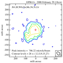
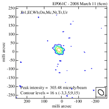
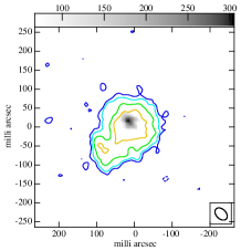
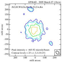
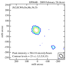
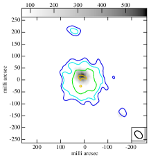
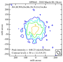
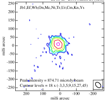
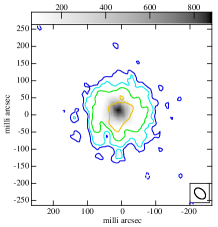
Figure 2: IRAS 23365 at L-band (left: 2, 2, 2), C-band (middle: 2, 2, 2), and L-band contours overlaid on grey scale C-band images (right: 2, 2, 2), in three different epochs (top to bottom), with the grey scale in  $\mathrm{\mu Jy}$ ranging from 3$\sigma$ value of the noisiest map in C-band (second epoch, i.e., $\sigma=23\,\mbox{$\mathrm{\mu Jy/beam}$}{}$), up to the peak intensity value of each epoch at C-band. Dashed contours represent $-3\sigma$ levels. All the images have been degraded to the epoch with lowest resolution (L2, following the labels in Table 2), being therefore convolved with the same beam size: 26$\times$38 mas² at 46°. The maps are centred at 23^h39^m01$\aas@@fstack{s}$29, +36°21′08$\aas@@fstack{\prime\prime}$59 (J2000). At the top of each image, we provide the EVN project code, observation date, observed wavelength and the list of antennas used for mapping. In the lower left corner we show the peak intensity, noise and contour levels information. The size of the nuclear region seems to increase from one epoch to another at both frequencies, although images from the same frequency were convolved with the same beam. We consider that this is an effect of the difference in the arrays used, rather than being an intrinsic change in the source, albeit this possibility cannot be neglected. It is worth noting that the size of the nuclear zone is consistently larger at L-band than its counterpart at C-band. This can be explained by the longer lifetime at lower frequencies of the electrons being accelerated in the innermost nuclear regions.

Table 3: EVN observational data, as measured from the images shown in Figure 2. Columns (2) and (3) Peak position coordinates given with respect to $\alpha(J2000)=23\mathrm{{}^{h}}39\mathrm{{}^{m}}01\aas@@fstack{s}0000$ and $\delta(J2000)=36\degr 21\arcmin 08\aas@@fstack{\prime\prime}000$. The errors in position (within parentheses), given in mas, were estimated by adding in quadrature the random errors in the position of the target (tar) and the phase reference calibrator (ref): $\sqrt[]{(\mathrm{FWHM}_{\mathrm{tar}}/(2\times SNR_{\mathrm{tar}}))^{2}+(\mathrm{FWHM}_{\mathrm{ref}}/(2\times SNR_{\mathrm{ref}}))^{2}}$, where $SNR$ is the signal to noise ratio, and FWHM was taken as the projection of the beam major axis on both $\alpha$ and $\delta$ axes. Column (4) rms noise in the maps. Column (5) Peak intensities. Column (6) Flux densities measured in regions enclosing 5$\sigma$ level of the emission. Column (7) Matched C-band flux densities, covering the 5$\sigma$ level L-band emission region; this is done by adding the C-band $S_{\mathrm{tot}}$ to a 3$\sigma$ emission in the remaining part. The uncertainties for the measurements shown in columns 5–7 have been estimated by adding in quadrature the rms noise in the map plus a 5 per cent uncertainty in the point source calibration. Column (8) Characteristic size (in both $\alpha$ and $\delta$) occupied by the emission at a 5$\sigma$ level.)

Label	$\Delta\alpha$(J2000)	$\Delta\delta$(J2000)	rms	$S_{\mathrm{peak}}$	$S_{\mathrm{tot}}$	$S_{\mathrm{match}}$	$R_{\alpha}\times R_{\delta}$
	(s)	(″)	( $\mathrm{\mu Jy/beam}$)	( $\mathrm{\mu Jy/beam}$)	( $\mathrm{mJy}$)	( $\mathrm{mJy}$)	(pc2)
(1)	(2)	(3)	(4)	(5)	(6)	(7)	(8)
L1	0.2600 (0.5)	0.592 (0.5)	28	786 $\pm$ 48	7.99 $\pm$ 0.40	$\cdots$	207 $\times$ 221
C1	0.2614 (0.7)	0.603 (0.7)	16	303 $\pm$ 22	0.32 $\pm$ 0.02	1.33 $\pm$ 0.07	68 $\times$ 69
L2	0.2616 (0.7)	0.598 (0.7)	25	466 $\pm$ 34	5.42 $\pm$ 0.27	$\cdots$	221 $\times$ 220
C2	0.2607 (0.5)	0.603 (0.5)	23	584 $\pm$ 37	1.11 $\pm$ 0.06	2.38 $\pm$ 0.12	98 $\times$ 94
L3	0.2615 (0.6)	0.566 (0.6)	30	640 $\pm$ 44	8.54 $\pm$ 0.43	$\cdots$	241 $\times$ 259
C3	0.2608 (0.3)	0.599 (0.3)	18	875 $\pm$ 47	2.45 $\pm$ 0.13	3.52 $\pm$ 0.18	111 $\times$ 127

All the epochs were VLBI phase-referenced experiments using a data recording rate of 1024 Mbps with two-bit sampling, for a total bandwidth of 128 MHz. The telescope systems recorded both right-hand circular polarization (RCP) and left-hand circular polarization (LCP). The data were correlated at the EVN MkIV Data Processor at JIVE using an averaging time of 2 s in the first two epochs, and 4 s in the third one, since there was no need for a field of view (FOV) as large as 20 arcsec. The sources 2134$+$004 and 3C45$4.3$ were used as fringe finders in all the observations. Each epoch lasted 6 hr, from which a total of $\approx 3.7$ hr were spent on target. Target source scans of 3.5 min were alternated with 1.5 min scans of the phase reference source.

The correlated data of every epoch were analysed using the NRAO Astronomical Image Processing System (AIPS). The overall quality of the visibilities was good and the EVN pipeline products were useful for the initial steps of the data reduction. To improve the calibration, we edited the data to remove artifacts due to radio interference (RFI) and included ionospheric corrections where needed. We exported the data of all the calibrators to the Caltech program DIFMAP (Shepherd et al., 1995) and made images and visibility plots of each source. This allowed us to test the performance of each antenna and to determine gain corrections for each. When the gain correction was larger than 10 per cent for a given antenna during the whole observing run, we applied it to the uv-data using the AIPS task CLCOR.

In the first two epochs we used J2333$+$3901 (at 2.9$\degr{}$ angular distance of target) as a phase reference source. This source has a complex structure (see Figure 1) and it varied in flux density at L-band between epochs (see column 7 in Table 2). The subtraction of the phase contribution due to the structure of J2333$+$3901 from the fringe solutions (delay and rate) was thus necessary. In spite of this correction, the phase referencing of the target source resulted in noisy phases.

In the third epoch we used J2330$+$3348 (at 3.1$\degr{}$ angular distance of our target) as a phase calibrator, which being a predominantly compact source (at mas angular scales) provided a reliable phase reference and calibration. To correct the reference position in our first two epochs, and to align the three observing epochs, we obtained the shifts in right ascension and declination for the first two epochs that make their 15$\sigma$ emission coincide positionally with the 15$\sigma$ emission of the third epoch. We did this by means of the task UVSUB in AIPS, in which the data was divided by a point source model of 1 Jy at the wanted reference position.

Figure 1: EVN contour maps of the phase reference source J2333$+$3901 at L-band, first 1 and second epoch 1.

3.1 Imaging process

The extended emission of IRAS 23365 is not completely resolved with the available EVN array. The shortest baselines, such as Ef-Wb, can recover some of the extended emission. If no other short baselines are present (e.g. combinations of Jb, Cm and Kn), it is not possible to determine closure phases, and the presence of strong sidelobes (of the order of the peak) in the dirty map is thus favoured. This situation made it very difficult to obtain a reliable image of the target source (see the preliminary maps of IRAS 23365 presented in Romero-Canizales et al., 2008). In principle, removing such short baselines would solve the problem, at the expense of significantly degrading the final image sensitivity.

To properly map the extended emission, a good coverage of short baselines (resulting from combinations of at least three antennas to determine closure phases) is needed. To overcome the lack of short uv-spacings, a combination of Gaussian model fitting and imaging algorithms can be used. This is a widely used method for mapping the structure of outflows at VLBI scales (see e.g., Rastorgueva et al., 2011), specially for the cases in which faint diffuse emission is present together with the bright compact one. Epochs 1 and 2 were affected by poor short-baseline uv-coverage (the Cm-Kn baseline had a severe amplitude problem and it was not used). In epoch 3, baselines Jb-Kn, Jb-Cm, Cm-Kn and Ef-Wb were present, thus permitting to determine closure phases for the short baselines. As a result, no strong sidelobes affected the imaging process at this epoch. Nevertheless, for this epoch we also used a Gaussian model fitting combined with clean components in order to obtain consistent results with those of the first two epochs. This was done within the Caltech imaging programme DIFMAP (Shepherd et al., 1995). We exported the resulting images back into AIPS to analyse them and to produce the final maps that we present here (see Figure 2).

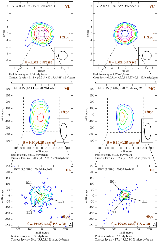
Figure 3: IRAS 23365 as seen at different frequencies and resolutions (higher resolution from top to bottom; and higher frequency from left to right, see labels). All the maps are centred at 23^h39^m01$\aas@@fstack{s}$29, +36°21′08$\aas@@fstack{\prime\prime}$59 (J2000). Dashed contours represent $-3\sigma$ levels. The cross in the EL image indicates the peak position (EC1) as measured from the EC image, and the crosses in the EC image indicate the positions of components EL1 and EL2. The non-coincidence of the peaks at the two different frequencies (see also ML and MC images), indicates the presence of distinct population of sources in the innermost nuclear region. We note that at C-band, IRAS 23365 remains practically unresolved, whilst L-band images show more extended structure.

In Table 2 we show the stations that participated in each observation. For different reasons, we lost some antennas and/or baselines and the final images were produced using the visibilities resulting from slightly different arrays. For instance, in the second epoch we lost Ur and Ar, and thus the resolution was compromised by the loss of the longest baselines. On the other hand, in the third epoch we had a good coverage of the short baselines (from combinations of Cm, Kn, Jb, Ef and Wb), which eased the reconstruction of the extended emission. To allow comparisons among the different epochs and frequencies, we used the same convolving beam (that from the epoch with the worst resolution: 26$\times$38 mas² at 46°) for the imaging process and sampled the beam using the same cell size ($=4$ mas), and natural weighting for all epochs. The resulting images for the three EVN epochs at the two different frequencies (1.7 and 5 GHz) are shown in Figure 2. The actual array used in the different epochs, is shown in a label at the upper right corner of each image. In Figure 3 (bottom) we also show the third EVN epoch at both 1.7 and 5 GHz, as imaged with the natural beam of the observation at 1.7 GHz (19$\times$25 mas² at 30°).

4 MERLIN and VLA observations

Simultaneously with our second EVN epoch, we also observed IRAS 23365 at both L- and C-bands with MERLIN (see Table 4), including the following antennas: Defford, Cambridge, Knockin, Darnhall, Mark 2 and Pickmere, observing with a bandwidth of 15 MHz (in both circular polarisations). OQ208 was used as amplitude calibrator (1.1 Jy at L-band and 2.5 Jy at C-band) and J2333$+$3901 (0.8 Jy at L-band and 0.34 Jy at C-band) as phase calibrator. For phase-referencing, duty times of 7 min/1.5 min in L-band, and 2.5 min/1.5 min in C-band were used, for a total time on source of 4 and 2.5 hr at each band, respectively.

We also analysed archival VLA (A-configuration) data at L- and C-bands (project: AB660, reported in Baan & Klöckner, 2006) to compare with the MERLIN and EVN images. The observations were performed with a bandwidth of 50 MHz (in both circular polarisations). 3C48 (16.0 Jy at L-band and 5.4 Jy at C-band) was the flux calibrator and 0025$+$393 (0.7 Jy and 0.6 Jy at L- and C-band, respectively) the phase calibrator, which is found at 9.6° angular distance of the target source.

We followed standard procedures within AIPS for the data reduction. Details on the VLA and MERLIN observations are shown in Table 4 and the resulting images in Figure 3. We used matched baselines (in wavelengths) to obtain the images for the two different frequencies of each array, to enable the comparison of information at the same scales. For the VLA images we used a common uv-range of 11.5 to 162.7 k$\lambda$ and same convolving beam of $1.3\times 1.3$ arcsec², while we restricted MERLIN images to 112.6 to 1191.8 k$\lambda$, that resulted in a convolving beam of $0.10\times 0.25$ arcsec², at 30$\degr{}$. We did not perform any uv-restriction in the case of the EVN data, to optimize the sensitivity and uv-coverage for each observing epoch.

Table 4: Parameters and observational data of complementary VLA and MERLIN observations (see the corresponding contour maps in Figure 3). The observations are labelled with a two-letter code, in which the first letter corresponds to the array (V$=$VLA or M$=$MERLIN), and the second letter to the observed frequency band (Column 3). Columns (4) and (5) Coordinates of the peak position, given with respect to $\alpha(J2000)=23\mathrm{{}^{h}}39\mathrm{{}^{m}}01\aas@@fstack{s}0000$ and $\delta(J2000)=36\degr 21\arcmin 08\aas@@fstack{\prime\prime}000$. Column (6) - rms noise in the maps. Column (7) Peak intensities. Column (8) Flux densities measured in regions enclosing 5$\sigma$ level of the emission. The uncertainties for the measurements shown in columns 4–5 and 7–8 have been estimated as described in Table 3. Column (9) Major and minor axes, obtained by fitting a Gaussian to the source. Column (10) Characteristic size (in both $\alpha$ and $\delta$) occupied by the emission at a 5$\sigma$ level.

Label	Observing	Freq.	$\Delta\alpha$(J2000)	$\Delta\delta$(J2000)	rms	$S_{\mathrm{peak}}$	$S_{\mathrm{tot}}$	$\Theta_{\mathrm{M}}\times\Theta_{\mathrm{m}}$	$R_{\alpha}\times R_{\delta}$
	date	(GHz)	(s)	(″)	( $\mathrm{\mu Jy/beam}$)	( $\mathrm{mJy/beam}$)	( $\mathrm{mJy}$)	(arcsec2)	(kpc2)
(1)	(2)	(3)	(4)	(5)	(6)	(7)	(8)	(9)	(10)
VL	1992-12-14	1.4	0.252 (6.1)	0.54 (6.1)	180	19.14 $\pm$ 0.97	25.18 $\pm$ 1.27	0.93 $\times$ 0.58	4.48 $\times$ 4.38
VC	1992-12-14	4.9	0.261 (3.3)	0.59 (3.3)	50	9.97 $\pm$ 0.21	10.82 $\pm$ 0.54	0.46 $\times$ 0.30	4.54 $\times$ 4.16
ML	2009-03-06	1.6	0.260 (1.6)	0.55 (4.0)	200	6.29 $\pm$ 0.37	13.90 $\pm$ 0.72	0.17 $\times$ 0.14	0.36 $\times$ 0.66
MC	2009-02-25	5.0	0.264 (3.6)	0.56 (8.9)	170	2.39 $\pm$ 0.50	5.20 $\pm$ 0.31	0.17 $\times$ 0.16	0.32 $\times$ 0.54

Table 5: Physical quantities of IRAS 23365 estimated from VLA, MERLIN and EVN observations. We have used the measured values of $S_{\mathrm{peak}}$, $S_{\mathrm{tot}}$ and the largest linear size between $R_{\alpha}$ and $R_{\delta}$, from Tables 3 and 4. In the case of the EVN, we only include the third epoch of observations, re-imaged with a convolving beam of 19$\times$25 mas² at 30° (see Figure 3). We consider the emission at both bands as measured from the region delimited by the 5$\sigma$ L-band emission, i.e., using $S_{\mathrm{tot}}$ for L-band, and $S_{\mathrm{match}}$ for C-band, and the same linear size for both. Column (2) Brightness temperature calculated using as the source’ solid angle $\Omega_{\mathrm{s}}=\pi(4\mathrm{log}2)^{-1}\left(\Theta_{\mathrm{M}}\times\Theta_{\mathrm{m}}\right)$ for the VLA and MERLIN (Table 4); for the EVN no reliable Gaussian fit can be made to the source (especially in the L-band map) in order to find its deconvolved size, and we have used instead $\Omega_{\mathrm{s}}=\pi(4\mathrm{log}2)^{-1}\left(\mathrm{FWHM}_{\mathrm{M}}\times\mathrm{FWHM}_{\mathrm{m}}\right)$, where $\mathrm{FWHM}_{\mathrm{M}}$ and $\mathrm{FWHM}_{\mathrm{m}}$ are the major and minor synthesized beam fitted FWHM. Column (3) Monochromatic luminosity at the frequency $\nu$. Column (4) Two-point peak pixel-to-pixel spectral index determined from the pixel-to-pixel spectral index distribution obtained with AIPS. Column (5) Two-point total spectral index determined between the L- and C-band flux densities ($S_{\mathrm{tot}}{}\propto\nu^{\alpha_{\mathrm{tot}}^{\mathrm{\mbox{\tiny L-C}}}}$). Column (6) Integrated isotropic radio luminosity, considering that the spectral behaviour of the source is straight between L- and C-band. Column (7) Equipartition magnetic field. Column (8) Characteristic lifetime of electrons subject to $B_{\mathrm{eq}}$, undergoing radiative synchrotron losses.

Label	log $T_{\mathrm{B}}$	$L_{\nu}$	$\alpha_{\mathrm{\mbox{\tiny p-p}}}^{\mathrm{\mbox{\tiny L-C}}}$	$\alpha_{\mathrm{tot}}^{\mathrm{\mbox{\tiny L-C}}}$	$L_{\mathrm{R}}$	$B_{\mathrm{eq}}$	$\tau_{\mathrm{syn}}$
	(K)	($10^{29}$$\,\mathrm{erg\,s^{-1}\,Hz^{-1}}$)			($10^{39}$ $\,\mathrm{erg\,s^{-1}}$)	($\mu$G)	(Myr)
(1)	(2)	(3)	(4)	(5)	(6)	(7)	(8)
VL	4.45 $\pm$ 0.02	19.11 $\pm$ 0.97				18.4	11.4
VC	3.61 $\pm$ 0.02	8.21 $\pm$ 0.41	-0.46 $\pm$ 0.06	-0.69 $\pm$ 0.06	4.1	18.1	6.2
ML	5.42 $\pm$ 0.02	10.55 $\pm$ 0.55				77.1	1.1
MC	3.96 $\pm$ 0.03	3.95 $\pm$ 0.24	-0.66 $\pm$ 0.13	-0.89 $\pm$ 0.07	2.0	90.8	0.6
EL	6.81 $\pm$ 0.02	4.94 $\pm$ 0.25				174.7	0.4
EC	5.57 $\pm$ 0.02	2.58 $\pm$ 0.13	0.52 $\pm$ 0.13	-0.59 $\pm$ 0.06	1.1	174.7	0.2

5 Results

IRAS 23365 has been observed at different resolutions (EVN, MERLIN and VLA) and at two different frequencies. This allows a comparison among the different linear scales mapped with different arrays. In the following, we present our results regarding morphology, radio emission, radio spectrum and magnetic field of IRAS 23365. The different parameters measured from the three epochs of EVN observations (see Figure 2) are presented in Table 3, and measurements from the VLA archival data and the MERLIN observations are presented in Table 4. In Table 5 we show the estimates from the measurements at different scales as shown in Figure 3.

5.1 The IRAS 23365 structure: from kpc- down to pc-scales

The radio images of IRAS 23365 shown in Figure 3, cover the structure of this galaxy at three different scales: galactic (with the VLA), circumnuclear (with MERLIN) and nuclear (with the EVN). We use the third epoch of EVN observations to compare with the VLA and MERLIN images, since that was the epoch with the best compromise between angular resolution and sensitivity (see Section 3.1 for details). For doing this, we re-imaged the third EVN epoch (L- and C-band maps) using as convolving beam that one which resulted from the L-band (19$\times$25 mas² at 30°, see bottom of Figure 3).

At galactic scales, the emission at both L- and C-bands is unresolved and appears concentrated in a zone of $\sim 4.5$ kpc in size. At circumnuclear scales, the emission is concentrated in the inner 0.5 kpc region and displays some extended structure on top of an unresolved component.

At the highest resolution in L-band, the nuclear region has a size $\ga$200 pc at all the EVN epochs (see Table 3), and shows variations in its morphology (see Figure 2). At C-band, the emitting region is about 100 pc and its structure remains quite compact in the first two epochs, whilst some more extended emission is traced in the third epoch (see Figure 2). A single Gaussian fit is inaccurate for obtaining the deconvolved size of the emitting region, at least for the emission at L-band, due to the wealth of extended emission. We thus characterize the area of the emitting region with the size of the source in both the right ascension and declination axes, $R_{\alpha}$ and $R_{\delta}$, respectively (Table 3). There are some features outside the nuclear regions that, while having peaks slightly above $5\sigma$ in our second epoch (Figures 2 and 2), are not seen neither in our first epoch, nor in our third observing epoch. While these could be real features (in particular, the compact source detected at both frequencies with $\Delta\alpha$, $\Delta\delta\sim 150$ mas), we conservatively consider them as tentative detections (see Section 3.1 for details) and therefore are not discussed here.

We note that the size of the emission area increases with time through the different EVN epochs at both frequencies (see Table 3), and also displays different morphology (see Figure 2), especially at L-band. Whereas sensitivity does not seem to vary drastically among epochs, the observations were performed at different hour angles and thus the uv-plane was sampled at different orientations. Hence, the differences in size and morphology could have been affected by the different uv-coverages.

Regardless of the used array (i.e., VLA, MERLIN or EVN), and albeit of using matched baselines (at least for VLA and MERLIN), the emission in L-band consistently occupies a larger extension than that at C-band, around a factor of 2 in the case of the EVN, as seen in Figure 3, where we show for comparison the VLA, MERLIN and EVN (third epoch) images. This can be explained by the longer lifetime of accelerated electrons emitting synchrotron radiation at lower frequencies (see Section 5.4).

We also note that the peak positions at the two different frequencies are not coincident neither for MERLIN nor for the EVN. In the case of the VLA, we do not have the required angular resolution to confirm any shift; however, at the higher resolution provided by both MERLIN and EVN, a shift of the C-band peak towards the North-East direction is evident, while that at L-band is shifted towards the South-West (see Tables 3 and 4 and Figure 3). This result is consistent for all the epochs and at the different angular resolutions provided by EVN and MERLIN. We interpret those shifts of the emission peaks as evidence for at least two different populations of radio emitters being present in the nuclear region (see Section 5.2). Furthermore, the peak component is variable both in position and in intensity among EVN epochs, and in each epoch, being also different between frequencies. These facts give evidence of the source variability within the innermost nuclear region.

5.2 The radio emission and radio spectrum at different scales

We mentioned in the previous section that the radio emission at different frequencies seen at the different resolutions (except perhaps for the VLA), peaks at different positions. Thus, a peak spectral index defined as $S_{\mathrm{peak}}{}\propto\nu^{\alpha_{\mathrm{peak}}^{\mathrm{\mbox{\tiny L-C}}}}$ would be meaningless. We use instead the peak of the pixel-to-pixel spectral index distribution ($\alpha_{\mathrm{\mbox{\tiny p-p}}}^{\mathrm{\mbox{\tiny L-C}}}$) as obtained with AIPS.

The radio emission of both galactic and circumnuclear regions of IRAS 23365 mapped with the VLA and MERLIN, respectively, is stronger at L-band than at C-band (see columns 7 and 8 in Table 4). Consequently both total spectral indices ($S_{\mathrm{tot}}{}\propto\nu^{\alpha_{\mathrm{tot}}^{\mathrm{\mbox{\tiny L-C}}}}$) and peak pixel-to-pixel spectral indices ($\alpha_{\mathrm{\mbox{\tiny p-p}}}^{\mathrm{\mbox{\tiny L-C}}}$) are steep, as shown in columns 4 and 5 of Table 5. Steep spectral indices are an indication of non-thermal emission. We note however that the $T_{\mathrm{B}}$ values (column 2 in Table 5) at galactic (L- and C-bands) and circumnuclear (C-band) scales, are in principle consistent with either thermal emission, or with synchrotron emission suppressed by free-free absorption from e.g., HII regions. The calculated value for the free-free opacity ($\tau_{\mathrm{ff}}$) implies that thermal emission should be optically thick. Therefore, the bulk of emission at L- and C-bands corresponds to optically thin non-thermal synchrotron emission, slightly affected by free-free absorption at galactic ($\tau_{\mathrm{ff}}\approx 0.02$) and circumnuclear ($\tau_{\mathrm{ff}}\approx 0.20$) scales.

Regarding the nuclear region (mapped with the EVN), the large $T_{\mathrm{B}}$ values are consistent with pure non-thermal emission. The attained angular resolution and the presence of strong extended (a few mJy; see Tables 3, and 4) radio emission, prevents us from directly detecting individual faint (see Table 1) compact sources, e.g. SNe. However, we note that $S_{\mathrm{peak}}$ and $S_{\mathrm{tot}}$ show variations at both frequencies during our EVN monitoring campaign (see Table 3). Whereas in C-band, $S_{\mathrm{peak}}$ and $S_{\mathrm{tot}}$ increase with time, in L-band these diminish in the second epoch, and then increase in the third one, thus indicating the variability of sources and/or the appearance of new ones within the nucleus, e.g., new SNe, accounting to the expected SN rate ($\approx 2.4$ yr^-1). This non-correlated behaviour at both frequencies is indicative of nuclear activity that becomes transparent first at C-band and later at L-band.

5.3 Spectral index distribution at mas-scales

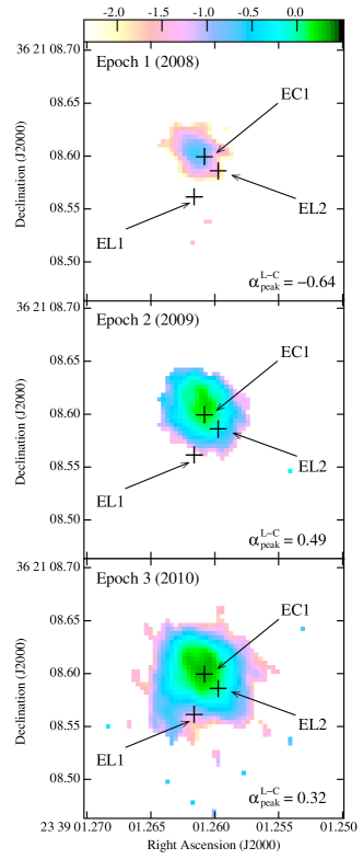
Figure 4: Evolution of the spectral index distribution ($S_{\mathrm{pixel}}\sim\nu^{\alpha_{\mathrm{\mbox{\tiny p-p}}}^{\mathrm{\mbox{\tiny L-C}}}}$), given pixel by pixel (as obtained from AIPS) in the nuclear zone, which we expect to be composed by non-thermal sources (e.g. SNe and AGN). Note that while the peak of the spectral index distribution varies in the very central region, it becomes steeper towards the edges, thus representing older radio emission. The sources EC1, EL1 and EL2 are marked with crosses (see Section 5.5).

Let us now concentrate in the spectral indices corresponding to the EVN images. Considering the total flux densities as measured from the region within the 5$\sigma$ L-band emission (i.e. L-band flux from column 6, and C-band flux from column 7 in Table 3), the total spectral indices ($\alpha_{\mathrm{tot}}^{\mathrm{\mbox{\tiny L-C}}}$) are steep for all the epochs. However, the situation is different for the peak pixel-to-pixel spectral index ($\alpha_{\mathrm{\mbox{\tiny p-p}}}^{\mathrm{\mbox{\tiny L-C}}}$), which is evolving with time. The distribution of $\alpha_{\mathrm{\mbox{\tiny p-p}}}^{\mathrm{\mbox{\tiny L-C}}}$ is shown in Figure 4 for the three EVN epochs. In the first epoch of EVN observations, $\alpha_{\mathrm{\mbox{\tiny p-p}}}^{\mathrm{\mbox{\tiny L-C}}}$ is steep, then it becomes inverted in our second epoch, and starts to decrease (although being still inverted) in the third epoch to presumably become steep again. This is clear evidence of the variation in flux of sources within the innermost nuclear regions, and/or appearance of new sources (e.g., SNe) which would be seen first at higher frequencies and later on at lower frequencies (Weiler et al., 2002), in agreement with our results. We also note that for the three EVN epochs, $\alpha_{\mathrm{\mbox{\tiny p-p}}}^{\mathrm{\mbox{\tiny L-C}}}$ (which is given pixel by pixel as shown in Figure 4), becomes steeper as measured towards the edges of the C-band emission, where the noise at C-band starts to dominate, whilst there is still extended emission detected at L-band. This is a consequence of the ageing of the population of electrons radiating synchrotron emission (see Section 5.4).

5.4 The magnetic field in the energy budget of IRAS 23365

In previous sections, we have gathered information about the ongoing non-thermal activity of IRAS 23365 at different scales. In a ULIRG environment, we expect SNe, SNRs and/or an AGN to be the engines responsible for producing high energy particles which will interact with the galactic magnetic field, thus generating synchrotron radiation (dominating at $\nu\la 30$ GHz; Condon, 1992). The energy thus produced, will be present in the form of relativistic particles and magnetic field. In the following, we investigate the energy budget (due to synchrotron radiation) of IRAS 23365 at different scales, i.e., as estimated from observations with different arrays (EVN, MERLIN and VLA). We only consider the third epoch of observations with the EVN, to compare with the results from the VLA and MERLIN, since this epoch was the one which had the least imaging problems (see Section 3.1).

We can estimate the average equipartition magnetic field based on the radio emission of IRAS 23365 as follows (see Pacholczyk, 1970),

$$\left(\frac{B_{\mathrm{eq}}}{\mu\mathrm{G}}\right)\approx 8.1\left[\frac{(1+k)}{\phi}\left(\frac{c_{\mbox{\tiny 12}}}{10^{7}}\right)\left(\frac{R}{1\,\mathrm{kpc}}\right)^{-3}\left(\frac{L_{\mathrm{R}}}{10^{39}\,\,\mathrm{erg\,s^{-1}}{}}\right)\right]^{2/7}$$ (2)

where $\phi$ is the filling factor of fields and particles, $k$ is the ratio of heavy particle energy to electron energy, and $c_{\mbox{\tiny 12}}$ is a function that depends on the minimum and maximum frequencies considered, and of the two-point spectral index, $\alpha_{\mathrm{tot}}^{\mathrm{\mbox{\tiny L-C}}}$, which is estimated based on those two frequencies (see Pacholczyk, 1970). $L_{\mathrm{R}}$ is the integrated isotropic radio luminosity between the minimum and maximum frequencies used, and $R$ is the linear size occupied by the emission, taken as the larger value between $R_{\alpha}$ and $R_{\delta}$ in each case (see column 10 in Table 4 for the VLA and MERLIN). For the third EVN epoch, we determined a maximum linear size $R\approx 0.2$ kpc with TVDIST within AIPS. For simplicity, we consider $\phi=0.5$ and $k=100$ (see e.g., Pérez-Torres & Alberdi, 2007).

In Table 5 we show the average values for $\alpha_{\mathrm{tot}}^{\mathrm{\mbox{\tiny L-C}}}$, $L_{\mathrm{R}}$ and $B_{\mathrm{eq}}$, obtained within the emission regions sampled by the different instruments. In the innermost nuclear region (imaged with the EVN), the strength of the magnetic field is larger than the one measured at lower resolutions. This is expected, since the plasma in the central regions should be denser than in the outer regions, and thus the magnetic field lines therein, frozen within the plasma, should be more concentrated. The average magnetic field under energy equipartition, for the emission measured with the VLA, MERLIN and the EVN, would be 18, 84 and 175 $\mu$G respectively. The latter value represents the peak of $B_{\mathrm{eq}}$ coming from the very central region. If the synchrotron spectrum holds beyond the C-band frequencies, e.g. to 20 GHz, the estimated values for $B_{\mathrm{eq}}$, would only be $\sim 15$ per cent larger.

Our obtained $B_{\mathrm{eq}}$ value at galactic scales is consistent with that of a galaxy in advanced interaction state, probably close to nuclear coalescence, according to VLA studies of interacting galaxies by Drzazga et al. (2011). Likewise, the $B_{\mathrm{eq}}$ value at nuclear scales is similar to that found through VLBI studies of the ULIRG IRAS 17208-0014 (144 $\mu$G; Momjian et al., 2003), which is also an advanced merger.

Considering the obtained values for $B_{\mathrm{eq}}$, and following Pacholczyk (1970), we can calculate the lifetime of the electrons with energy $E_{\mathrm{min}}$, which move in a magnetic field of strength $B_{\mathrm{eq}}$, thus emitting synchrotron radiation around a critical frequency $\nu_{\mathrm{c}}$. This is,

$$\tau_{\mathrm{syn}}=\frac{1}{c_{2}E_{\mathrm{min}}B_{\mathrm{eq}}^{2}},$$

(where $c_{\mbox{\tiny 2}}$ is a constant)

$$\Rightarrow\left(\frac{\tau_{\mathrm{syn}}}{\mathrm{Myr}}\right)\approx 1.06\times 10^{3}\left[\left(\frac{\nu_{\mathrm{c}}}{\mathrm{GHz}}\right)\left(\frac{B_{\mathrm{eq}}}{\mu\mathrm{G}}\right)^{3}\right]^{-1/2}$$ (3)

Table 6: Parameters derived for the compact components EC1, EL1 and EL2 found within the extended emission in the third epoch of EVN observations (Figure 3). Columns (2) and (3) Coordinates of the peak position, given with respect to $\alpha(J2000)=23\mathrm{{}^{h}}39\mathrm{{}^{m}}01\aas@@fstack{s}0000$ and $\delta(J2000)=36\degr 21\arcmin 08\aas@@fstack{\prime\prime}000$. Column (4) Peak intensity corrected by the zero level emission. Column (5) Monochromatic luminosity. Column (6) Brightness temperature, considering that the solid angle subtended by the source is that subtended by the synthesized beam (as in Table 5).

Label	$\Delta\alpha$(J2000)	$\Delta\delta$(J2000)	$S_{\mathrm{peak}}$	$L_{\nu}$	log $T_{\mathrm{B}}$
	(s)	(″)	( $\mathrm{\mu Jy/beam}$)	($10^{28}$$\,\mathrm{erg\,s^{-1}\,Hz^{-1}}$)	(K)
(1)	(2)	(3)	(4)	(5)	(6)
EC1	0.2608 (0.4)	0.599 (0.4)	352 $\pm$ 35	2.67 $\pm$ 0.26	4.56 $\pm$ 0.04
EL1	0.2597 (1.7)	0.586 (1.7)	150 $\pm$ 32	1.14 $\pm$ 0.24	5.15 $\pm$ 0.09
EL2	0.2616 (1.4)	0.561 (1.4)	184 $\pm$ 33	1.39 $\pm$ 0.25	5.23 $\pm$ 0.08

From Section 5.1, we know that the radio emission at L- and C-bands has a different extent and peaks at different positions within the nuclear region, which strongly suggests the presence of different populations of particles. This is more evident in the nuclear region mapped with the EVN: in the innermost region, where there is an overlap between the emission at the two different frequencies, there would be a concentration of very energetic, short-lived particles, whereas the outer region would be populated by less energetic, long-lived particles, which had had time to diffuse from the inner regions into the outer ones. In Table 5 we show the values for $\tau_{\mathrm{syn}}$, assuming that the critical frequency is either that of the L-band or the C-band. In all cases we see that the L-band emission is tracing the emission from an older population of electrons (regardless of the resolution) than the one emitting at C-band frequencies. The putative AGN together with an ensemble of SNe, for which evidence has been found in other studies (see Section 2.1), must be located within the C-band emission region as seen with the EVN, where the magnetic field strength is larger, and where a composite spectrum (which varies with time) has been found (Section 5.2).

We note that the radio lifetime of the emitting source is not only determined by $\tau_{\mathrm{syn}}$. The lifetime of relativistic electrons might also be affected by Compton losses given by

$$\tau_{\mathrm{C}}=\frac{25.2}{U_{\mathrm{rad}}E_{\mathrm{min}}},$$

(following Pacholczyk, 1970) since the electrons are immersed in a radiation field,

$$U_{\mathrm{rad}}=\frac{4\pi}{c}\frac{L_{\mathrm{bol}}}{\Omega_{\mathrm{s}}},$$

for which we take $L_{\mathrm{IR}}$ as a good approximation to the bolometric luminosity $L_{\mathrm{bol}}$. $U_{\mathrm{rad}}$ varies from $\approx 2.5\times 10^{-7}$ erg cm^-3 at galactic scales, up to $\approx 2.8\times 10^{-4}$ erg cm^-3 at nuclear scales. To compare the different losses, we calculate their ratio,

$$\tau_{\mathrm{C}}/\tau_{\mathrm{syn}}=\frac{25.2c_{2}B_{\mathrm{eq}}^{2}}{U_{\mathrm{rad}}}.$$

We note that at all scales (nuclear, circumncuclear and galactic) and at both L- and C-band, we obtain $\tau_{\mathrm{syn}}\gg\tau_{\mathrm{C}}$, with a ratio ranging between $6.5\times 10^{-6}$ (nuclear scales) and $8.8\times 10^{-5}$ (galactic scales); i.e., the energy density of the radiation field, greatly exceeds the magnetic energy density. Radiative losses are important and we argue that there is need for injection of new electrons or a continuous acceleration to halt the energy depletion, otherwise radio emission would not be visible.

The re-acceleration or injection of new electrons in a (U)LIRG environment, is very likely provided in SN-shells and SNRs by first order Fermi acceleration. The presence of SNe, SNRs and a strong magnetic field in IRAS 23365, agrees with this scenario.

5.5 The nuclear region in the third EVN epoch

Among the EVN observing epochs, the third one benefited from a better uv-coverage, and thus resulted in a smaller natural beam (19$\times$25 mas² at 30° at L-band). The L-band map (Figure 3, bottom-left) shows the presence of two compact sources (EL1 and EL2) within the nuclear region, without counterparts at C-band. On the other hand, the compact source that dominates the emission at C-band, labelled as EC1 (Figure 3, bottom-right), has no compact counterpart at L-band, although extended emission is present.

To obtain EC1, EL1 and EL2 peak intensities, we first estimated the background emission where these compact sources lay. We solved for the ’zero level’ emission ($S_{\mathrm{bg}}\sim 179\pm 24$  $\mathrm{\mu Jy}$ at C-band and $S_{\mathrm{bg}}\sim 211\pm 12$  $\mathrm{\mu Jy}$ at L-band) using the task IMFIT within AIPS. We then subtracted this value from the maximum intensity found at the positions of each compact source, in order to obtain their $S_{\mathrm{peak}}$. In Table 6 we give the positions for EC1, EL1 and EL2, their peak intensities, as well as their estimated $L_{\nu}$ and $T_{\mathrm{B}}$, which are indicative of a non-thermal origin.

EC1 lays on a region where $\alpha_{\mathrm{\mbox{\tiny p-p}}}^{\mathrm{\mbox{\tiny L-C}}}$ changes with time, suggesting variability within this region. We note that EC1 is confined to a small area in the first epoch, and then appears to increase in size, as we have mentioned in Section 5.1. EL1 lays in a region with basically no C-band emission, unlike the region where EL2 lays where more extended emission is being traced from the first epoch to the third one at C-band. As a consequence, EL1 lays in a region which maintains a very steep $\alpha_{\mathrm{\mbox{\tiny p-p}}}^{\mathrm{\mbox{\tiny L-C}}}$ through time, whilst EL2 is found in a region with varying $\alpha_{\mathrm{\mbox{\tiny p-p}}}^{\mathrm{\mbox{\tiny L-C}}}$ (Figure 4). However, we cannot rule out that the $\alpha_{\mathrm{\mbox{\tiny p-p}}}^{\mathrm{\mbox{\tiny L-C}}}$ variations at EL2 are intrinsic.

In the case of EC1, both the variability of the radio emission (see Section 5.2) and of the spectral index distribution (see Section 5.3 and Figure 4) are indicative of recent non-thermal activity (probably due to SNe and/or AGN activity). EL1 and EL2 display brightness temperatures similar to those expected from either type II SNe or SNRs. We note that the maximum linear size for EL1 and EL2 is set by the beam size to $\sim 30$ pc, which is too large for characterising either an individual SN or a SNR. A scenario in which EL1 and EL2 are clusters of SNe is difficult to reconcile with the absence of peaks of emission at C-band in all the EVN observing epochs, and with the behaviour of $\alpha_{\mathrm{\mbox{\tiny p-p}}}^{\mathrm{\mbox{\tiny L-C}}}$ at both EL1 and EL2. These facts suggest that there is no recent activity from young SNe in those regions, and favour an scenario in which EL1 and EL2 are dominated by an old population of radio emitters.

6 Summary and discussion

We have presented state-of-the-art radio interferometric images of IRAS 23365, one of the brightest and farthest ULIRGs in the local Universe ($z<0.1$).

Our images reveal the presence of a nuclear region, possibly a starburst-AGN composite, with an approximate size of 200 pc in L-band, and about 100 pc in C-band. We find that the L- and C-band radio emission peak at different positions, thus suggesting that the nuclear region is composed of at least two zones, dominated by distinct populations of radio emitters.

In the region where the L- and C-band emission overlap, there is evidence for ongoing non-thermal activity, characterised by very energetic, short-lived particles . During our EVN monitoring of IRAS 23365, we have found flux density variability in the overlapping region, thus resulting in a variation of the spectral index. This can be explained by the flux density variations of sources therein (SNe, AGN, etc.) and/or by the appearance of new sources (e.g., SNe) which would be seen first at higher frequencies and later at lower frequencies (Weiler et al., 2002). The edges of the overlapping region characterised by less energetic, long-lived particles, would be dominated by an old population of radio emitters, probably clumps of SNRs, for which we have found two candidates in the third L-band EVN epoch. These facts agree with the classification of IRAS 23365 as a composite system, made by Yuan et al. (2010).

The radio source lifetime at different scales (as seen with the VLA, MERLIN and the EVN arrays) and at both L- and C-bands, is limited by Compton losses. The SNe and SNRs, for which we have found evidence, are likely providing the mechanism of re-acceleration, or replenishment of new electrons that is needed to halt the radio energy depletion.

We have found that the equivalent magnetic field strength at galactic (mapped with the VLA) and nuclear scales (mapped with the EVN), 18 and 175 $\mu$G, respectively, correspond to that of a galaxy in an advanced stage of interaction (Drzazga et al., 2011; Momjian et al., 2003). The magnetic field in both nuclear and circumnuclear regions is stronger than at galactic scales, thus implying that the lifetime of the electrons undergoing synchrotron losses is shorter ($\la 1$ Myr) in the innermost nuclear regions (with linear size $R\la 0.5$ kpc) of IRAS 23365, and larger ($\ga 1$ Myr) in the outer regions ($R\ga 4$ kpc).

Our study of IRAS 23365 (at $z\sim 0.06$) has shown that high-resolution, high-sensitivity observations are needed if we are to make significant improvement in the detailed understanding of nuclear and circumnuclear starbursts in the local Universe. The resolution we attained using a maximum baseline length of approximately 7,000 km, is not enough to resolve individual compact sources (e.g., SNe, SNRs, AGN) from each other, within the nuclear region of IRAS 23365; yet, it could be possible to infer the activity of such compact sources, by carefully monitoring variations of total flux density and spectral index distribution. For instance, Romero-Cañizales et al. (2011) were able to directly detect SN activity in the B1-nucleus of Arp 299, by carefully monitoring the variations in $S_{\mathrm{tot}}$, over several years of VLA observations. Without spatially resolving each individual SNe, they estimated a lower limit for the $\nu_{\mathrm{\mbox{\tiny SN}}}$ in that LIRG. In the case of IRAS 23365, where a larger number of SNe are expected each year, several observations per year would be needed to perform such an indirect study of the SN population in its nuclear region, provided that we are able to distinguish between AGN outbursts and SN explosions.

IRAS 23365 is a good example of the situation to be faced when observing galaxies at higher redshifts. It is expected that the Square Kilometer Array (SKA), with a maximum baseline length $\approx 3,000$ km, will allow the detection of sources as faint as 50 nJy, e.g. CCSNe, exploding at $z\sim 5$ (see e.g., Lien et al., 2011). However, the angular resolution will be a strong limiting factor. In those cases where the nuclear and even the circumnuclear regions (i.e., where we expect most of the SN activity to occur) of the host galaxy cannot be resolved out into their different components, SKA’s high sensitivity might be of great use to indirectly detect SN activity through the monitoring of flux density variations.

References

- Alberdi et al. (2006) Alberdi A., Colina L., Torrelles J. M., Panagia N., Wilson A. S., Garrington S. T., 2006, ApJ, 638, 938
- Baan & Klöckner (2006) Baan W. A., Klöckner H.-R., 2006, A&A, 449, 559
- Caputi et al. (2007) Caputi K. I., Lagache G., Yan L., Dole H., Bavouzet N., Le Floc’h E., Choi P. I., Helou G., Reddy N., 2007, ApJ, 660, 97
- Carilli & Taylor (2000) Carilli C. L., Taylor G. B., 2000, ApJ, 532, L95
- Colina et al. (2001) Colina L., Alberdi A., Torrelles J. M., Panagia N., Wilson A. S., 2001, ApJ, 553, L19
- Condon (1992) Condon J. J., 1992, Annual Review of Astron and Astrophys, 30, 575
- Condon et al. (1990) Condon J. J., Helou G., Sanders D. B., Soifer B. T., 1990, ApJS, 73, 359
- Condon et al. (1996) Condon J. J., Helou G., Sanders D. B., Soifer B. T., 1996, ApJS, 103, 81
- Drzazga et al. (2011) Drzazga R. T., Chyży K. T., Jurusik W., Wiórkiewicz K., 2011, A&A, 533, A22+
- Farrah et al. (2003) Farrah D., Afonso J., Efstathiou A., Rowan-Robinson M., Fox M., Clements D., 2003, MNRAS, 343, 585
- Farrah et al. (2001) Farrah D., Rowan-Robinson M., Oliver S., Serjeant S., Borne K., Lawrence A., Lucas R. A., Bushouse H., Colina L., 2001, MNRAS, 326, 1333
- Iwasawa et al. (2011) Iwasawa K., Sanders D. B., Teng S. H., U V., Armus L., Evans A. S., Howell J. H., Komossa S., Mazzarella J. M., Petric A. O., Surace J. A., Vavilkin T., Veilleux S., Trentham N., 2011, A&A, 529, A106+
- Kewley et al. (2006) Kewley L. J., Groves B., Kauffmann G., Heckman T., 2006, MNRAS, 372, 961
- Klaas & Elsaesser (1991) Klaas U., Elsaesser H., 1991, A&AS, 90, 33
- Lien et al. (2011) Lien A., Chakraborty N., Fields B. D., Kemball A., 2011, ApJ, 740, 23
- Lilly et al. (1999) Lilly S. J., Eales S. A., Gear W. K. P., Hammer F., Le Fèvre O., Crampton D., Bond J. R., Dunne L., 1999, ApJ, 518, 641
- Mattila & Meikle (2001) Mattila S., Meikle W. P. S., 2001, MNRAS, 324, 325
- Mattila et al. (2007) Mattila S., Väisänen P., Farrah D., Efstathiou A., Meikle W. P. S., Dahlen T., Fransson C., Lira P., Lundqvist P., Östlin G., Ryder S., Sollerman J., 2007, ApJ, 659, L9
- Momjian et al. (2003) Momjian E., Romney J. D., Carilli C. L., Troland T. H., Taylor G. B., 2003, ApJ, 587, 160
- Neff et al. (2004) Neff S. G., Ulvestad J. S., Teng S. H., 2004, ApJ, 611, 186
- Pacholczyk (1970) Pacholczyk A. G., 1970, Radio Astrophysics: Nonthermal processes in galactic and extragalactic sources. W. H. Freeman and Company
- Parra et al. (2010) Parra R., Conway J. E., Aalto S., Appleton P. N., Norris R. P., Pihlström Y. M., Kewley L. J., 2010, ApJ, 720, 555
- Parra et al. (2007) Parra R., Conway J. E., Diamond P. J., Thrall H., Lonsdale C. J., Lonsdale C. J., Smith H. E., 2007, ApJ, 659, 314
- Pérez-Torres & Alberdi (2007) Pérez-Torres M. A., Alberdi A., 2007, MNRAS, 379, 275
- Pérez-Torres et al. (2009) Pérez-Torres M. A., Alberdi A., Colina L., Torrelles J. M., Panagia N., Wilson A., Kankare E., Mattila S., 2009, MNRAS, 399, 1641
- Pérez-Torres et al. (2010) Pérez-Torres M. A., Alberdi A., Romero-Cañizales C., Bondi M., 2010, A&A, 519, L5+
- Pérez-Torres et al. (2007) Pérez-Torres M. A., Mattila S., Alberdi A., Colina L., Torrelles J. M., Väisänen P., Ryder S., Panagia N., Wilson A., 2007, ApJ, 671, L21
- Pérez-Torres et al. (2009) Pérez-Torres M. A., Romero-Cañizales C., Alberdi A., Polatidis A., 2009, A&A, 507, L17
- Rastorgueva et al. (2011) Rastorgueva E. A., Wiik K. J., Bajkova A. T., Valtaoja E., Takalo L. O., Vetukhnovskaya Y. N., Mahmud M., 2011, A&A, 529, A2+
- Romero-Cañizales et al. (2011) Romero-Cañizales C., Mattila S., Alberdi A., Pérez-Torres M. A., Kankare E., Ryder S. D., 2011, MNRAS, 415, 2688
- Romero-Canizales et al. (2008) Romero-Canizales C., Perez-Torres M., Alberdi A., 2008, in The role of VLBI in the Golden Age for Radio Astronomy EVN observations of the Ultra Luminous Infrared Galaxies IRAS 23365+3604 and IRAS07251-0248
- Sanders et al. (2003) Sanders D. B., Mazzarella J. M., Kim D., Surace J. A., Soifer B. T., 2003, AJ, 126, 1607
- Sanders & Mirabel (1996) Sanders D. B., Mirabel I. F., 1996, Annual Review of Astron and Astrophys, 34, 749
- Sanders et al. (1988) Sanders D. B., Soifer B. T., Elias J. H., Neugebauer G., Matthews K., 1988, ApJ, 328, L35
- Shepherd et al. (1995) Shepherd M. C., Pearson T. J., Taylor G. B., 1995, in B. J. Butler & D. O. Muhleman ed., Bulletin of the American Astronomical Society Vol. 27 of Bulletin of the American Astronomical Society, DIFMAP: an interactive program for synthesis imaging.. pp 903–+
- Smith et al. (1998) Smith H. E., Lonsdale C. J., Lonsdale C. J., Diamond P. J., 1998, ApJ, 493, L17
- Sopp et al. (1990) Sopp H., Alexander P., Riley J., 1990, MNRAS, 246, 143
- Veron et al. (1997) Veron P., Goncalves A. C., Veron-Cetty M.-P., 1997, A&A, 319, 52
- Weiler et al. (2002) Weiler K. W., Panagia N., Montes M. J., Sramek R. A., 2002, Annual Review of Astron and Astrophys, 40, 387
- Yuan et al. (2010) Yuan T.-T., Kewley L. J., Sanders D. B., 2010, ApJ, 709, 884