On the interaction between tides and convection

Abstract

We study the interaction between tides and convection in astrophysical bodies by analysing the effect of a homogeneous oscillatory shear on a fluid flow. This model can be taken to represent the interaction between a large-scale periodic tidal deformation and a smaller-scale convective motion. We first consider analytically the limit in which the shear is of low amplitude and the oscillation period is short compared to the timescales of the unperturbed flow. In this limit there is a viscoelastic response and we obtain expressions for the effective elastic modulus and viscosity coefficient. The effective viscosity is inversely proportional to the square of the oscillation frequency, with a coefficient that can be positive, negative or zero depending on the properties of the unperturbed flow. We also carry out direct numerical simulations of Boussinesq convection in an oscillatory shearing box and measure the time-dependent Reynolds stress. The results indicate that the effective viscosity of turbulent convection falls rapidly as the oscillation frequency is increased, attaining small negative values in the cases we have examined, although significant uncertainties remain because of the turbulent noise. We discuss the implications of this analysis for astrophysical tides.

1 Introduction

Tidal interactions determine the orbital and spin evolution of astrophysical bodies when they orbit sufficiently close to one another. Applications include close binary stars, extrasolar planetary systems and the satellites of solar-system planets.

In many cases of interest the tidally forced bodies are fully or partly convective. In order to determine the rate of tidal evolution it is therefore necessary to study the interaction between tides and convection. The response of a fluid body to tidal forcing generally consists of two components: one is non-wavelike and of large scale, while the other involves internal waves of smaller scale. At the simplest level the convection could be thought of as providing an effective viscosity that damps the non-wavelike tidal disturbance and provides a phase shift in the response. As in the theory of Darwin (1880), the tidal torque and the rate of tidal evolution are then directly proportional to this effective viscosity. Convection may also play an important role in dissipating inertial waves, which constitute the low-frequency wavelike response of rotating convective zones of stars and giant planets (e.g. Ogilvie & Lin, 2004).

As pointed out by Zahn (1966) and Goldreich & Nicholson (1977), the effective viscosity estimated from mixing-length theory ought to be reduced when the period of the tidal disturbance is short compared to the characteristic timescale of the convective motion. The suppression factor has been the subject of much debate, informed by observational constraints such as the apparent rate of circularization of the orbits of close binary stars (Meibom & Mathieu, 2005, and references therein). Zahn (1966) suggested a less severe suppression, such that the effective viscosity is proportional to the oscillation period for short periods, which is in better agreement with these observations. Goldreich & Nicholson (1977) and Goldreich & Keeley (1977) considered the multiscale nature of the turbulent flow, and argued that the dominant contribution to the effective viscosity at short periods comes from eddies with a convective timescale comparable to the oscillation period. For a Kolmogorov spectrum, this argument gives a more powerful suppression, such that the effective viscosity is proportional to the square of the oscillation period for short periods.

While these authors relied on simple physical arguments and order-of-magnitude estimates, Goodman & Oh (1997), who also provide a clear review of the controversy, introduced a more formal procedure for determining the effective viscosity of a convective flow, by considering the effect of a homogeneous oscillatory strain on a turbulent velocity field. Analytical progress was limited by the complexity of the equations. While their method relies on an expansion in powers of the ratio of the oscillation period to the convective timescale, it leads to a result in which the dominant contribution comes from eddies for which these timescales are similar. Their argument does, however, appear to rule out the hypothesis of Zahn (1966).

More recently, numerical simulations of convection have been brought to bear on this question. Penev et al. (2007) and Penev et al. (2009) applied the procedure of Goodman & Oh (1997) to the velocity fields obtained in numerical simulations of convection in a deep layer, to deduce the effective viscosity as a function of the tidal frequency. In Penev, Barranco & Sasselov (2009) an oscillatory forcing was introduced directly into the convection simulation and the effective viscosity was estimated by measuring the work done by this force. The results of these studies suggest that something closer to the prescription of Zahn (1966) may be appropriate, not for the reasons originally suggested, but possibly because the power spectrum of the convection is less steep than the Kolmogorov spectrum assumed by Goldreich & Nicholson (1977).

While the results of Penev and collaborators are of considerable interest, the uncertainties in these calculations have not been quantified. Owing to the importance of this problem, we are motivated to examine it from an independent viewpoint. We have devised a theoretical framework that allows us to study statistically homogeneous flows; while this local viewpoint omits important global aspects of stellar or planetary convection, it allows us to resolve convection at high Rayleigh numbers and to quantify the uncertainties due to turbulent noise. We also present complementary analytical results which shed new light on previous theoretical discussions.

The plan of this paper is as follows. In Section 2 we introduce the homogeneous sheared coordinate system used in our analytical and numerical calculations, and discuss the equations of fluid dynamics in this system. In Section 3 we derive the response of a fluid flow to oscillatory shear in the limits of low amplitude and high frequency, and calculate the effective elasticity and viscosity in various cases. Direct numerical simulations of convection in an oscillatory shearing box are reported and interpreted in Section 4, followed by a summary and discussion of the results.

2 The oscillatory shearing box

2.1 Motivation

At the present time it is not practical to compute a global model of an astrophysical body with turbulent convection and to measure its tidal response through the direct application of a time-dependent gravitational potential. As noted in the introduction, the response of a fluid body to tidal forcing generally consists of a large-scale non-wavelike motion together with some internal waves. The non-wavelike tide can be computed without difficulty in a linear approximation and consists of a time-dependent spheroidal deformation of the body. From the local perspective of the smaller-scale convective motion, this tidal flow appears as a spatially homogeneous, approximately incompressible motion that is oscillatory in time. We are interested, therefore, in determining the response of the convective motion to such a deformation and the additional stresses that result from this interaction.

A general, three-dimensional, spatially homogeneous, incompressible deformation can be represented by a traceless velocity gradient tensor ${\mn@boldsymbol{\nabla}}{\mn@boldsymbol{u}}$ that is independent of position. In this paper we consider a time-dependent simple shear of the form $u_{y}\propto x$. Using a linear combination of simple shears with different orientations it is possible to compose an arbitrary velocity gradient tensor that is traceless (see Appendix A). Provided that we are working a linear regime, therefore, it is sufficient to measure the response to a time-dependent simple shear.

2.2 Sheared coordinates

We initially consider an incompressible fluid in two dimensions, satisfying the Navier–Stokes equations

$$(\partial_{t}+u_{x}\partial_{x}+u_{y}\partial_{y})u_{x}=-\partial_{x}p+\nu(\partial_{x}^{2}+\partial_{y}^{2})u_{x}+\tilde{f}_{x},$$ (1)

$$(\partial_{t}+u_{x}\partial_{x}+u_{y}\partial_{y})u_{y}=-\partial_{y}p+\nu(\partial_{x}^{2}+\partial_{y}^{2})u_{y}+\tilde{f}_{y},$$ (2)

$$\partial_{x}u_{x}+\partial_{y}u_{y}=0,$$ (3)

where ${\mn@boldsymbol{u}}$ is the velocity, $p$ is the pressure divided by the density, $\nu$ is the kinematic viscosity and $\tilde{\mn@boldsymbol{f}}$ is a body force per unit mass.

We suppose that the system is subject to a homogeneous time-dependent shear. We define the sheared coordinates

$$x^{\prime}=x,\qquad y^{\prime}=y-a(t)x,\qquad t^{\prime}=t.$$ (4)

The dimensionless quantity $a$ is the shear, and $\dot{a}=\mathrm{d}a/\mathrm{d}t$ is the shear rate. The Jacobian determinant of the transformation is unity. Partial derivatives transform according to

$$\partial_{x}=\partial_{x}^{\prime}-a\partial_{y}^{\prime},\qquad\partial_{y}=\partial_{y}^{\prime},\qquad\partial_{t}=\partial_{t}^{\prime}-\dot{a}x\partial_{y}^{\prime}.$$ (5)

We write

$$u_{x}=v_{x},\qquad u_{y}=v_{y}+\dot{a}x,$$ (6)

so that ${\mn@boldsymbol{v}}$ represents the velocity relative to the shearing motion. We continue to refer vector components to the original Cartesian basis.

With these substitutions, the Navier–Stokes equations become

$$[\partial_{t}^{\prime}+v_{x}(\partial_{x}^{\prime}-a\partial_{y}^{\prime})+v_{y}\partial_{y}^{\prime}]v_{x}=-(\partial_{x}^{\prime}-a\partial_{y}^{\prime})p+\nu\Delta v_{x}+\tilde{f}_{x},$$ (7)

$$\begin{split}&[\partial_{t}^{\prime}+v_{x}(\partial_{x}^{\prime}-a\partial_{y}^{\prime})+v_{y}\partial_{y}^{\prime}]v_{y}+\ddot{a}x^{\prime}+\dot{a}v_{x}=-\partial_{y}^{\prime}p\\ &\qquad+\nu\Delta v_{y}+\tilde{f}_{y},\end{split}$$

$$(\partial_{x}^{\prime}-a\partial_{y}^{\prime})v_{x}+\partial_{y}^{\prime}v_{y}=0,$$ (8)

involving the Laplacian operator in unsheared coordinates,

$$\begin{split}\Delta&=\partial_{x}^{2}+\partial_{y}^{2}\\ &=(\partial_{x}^{\prime}-a\partial_{y}^{\prime})^{2}+\partial_{y}^{\prime 2}\\ &=\Delta^{\prime}-2a\partial_{x}^{\prime}\partial_{y}^{\prime}+a^{2}\partial_{y}^{\prime 2}.\end{split}$$

These equations are spatially homogeneous (not involving $x^{\prime}$ or $y^{\prime}$ explicitly) except for the term $\ddot{a}x^{\prime}$, which arises because a spatially inhomogeneous force is required to maintain an accelerating shear. By writing

$$\tilde{f}_{x}=f_{x},\qquad\tilde{f}_{y}=\ddot{a}x^{\prime}+f_{y},$$ (9)

i.e. by subtracting the inhomogeneous force, we restore spatial homogeneity to the equations. In this representation, ${\mn@boldsymbol{f}}$ is the body force that, if necessary, drives the (possibly turbulent) motion whose response we wish to measure, while $\ddot{a}x^{\prime}\,{\mn@boldsymbol{e}}_{y}$ is the force that drives the imposed large-scale shear.

The property of spatial homogeneity results from the translational invariance of the homogeneously sheared system, given that a Galilean transformation easily removes the velocity shift associated with a translation in the $x$ direction. It means that statistically homogeneous turbulence, for example, is possible in this system. It also means that, for computational or analytical purposes, we can impose periodic boundary conditions on ${\mn@boldsymbol{v}}$ and $p$ in sheared coordinates. When employing a spectral method, these variables can be expanded in Fourier series in sheared coordinates, using basis functions $\exp(\mathrm{i}k_{x}^{\prime}x^{\prime}+\mathrm{i}k_{y}^{\prime}y^{\prime})$.

An alternative approach, which leads to identical results, is to solve the original equations in unsheared coordinates but to apply modified periodic boundary conditions of the form

$$p(L_{x},y,t)=p(0,(y-a(t)L_{x})\bmod L_{y},t),$$ (10)

$$p(x,L_{y},t)=p(x,0,t),$$ (11)

and similarly for ${\mn@boldsymbol{v}}$ (not ${\mn@boldsymbol{u}}$), where $L_{x}$ and $L_{y}$ are the dimensions of the shearing box. The appropriate basis is then one composed of shearing waves $\exp(\mathrm{i}k_{x}(t)x+\mathrm{i}k_{y}y)$, having (quantized) time-dependent wavevectors with components $k_{x}(t)=k_{x}^{\prime}-a(t)k_{y}^{\prime}$ and $k_{y}=k_{y}^{\prime}$. With these definitions, $\exp(\mathrm{i}k_{x}(t)x+\mathrm{i}k_{y}y)=\exp(\mathrm{i}k_{x}^{\prime}x^{\prime}+\mathrm{i}k_{y}^{\prime}y^{\prime})$.

Note that the oscillatory shear in our model is not imposed by the boundary conditions as such, but is driven by the inhomogeneous body force $\ddot{a}x^{\prime}\,{\mn@boldsymbol{e}}_{y}$ as described above. Our model therefore provides a self-consistent local representation of any turbulent flow subject to an oscillatory deformation due to an external body force.

Similar considerations apply to the Boussinesq equations in three dimensions, or indeed to the equations of compressible convection. In the Boussinesq case the basic equations in unsheared coordinates are

$$(\partial_{t}+u_{j}\partial_{j})u_{i}=-\partial_{i}p+\nu\Delta u_{i}+be_{i}+\tilde{f}_{i},$$ (12)

$$(\partial_{t}+u_{i}\partial_{i})b+N^{2}u_{i}e_{i}=\kappa\Delta b,$$ (13)

$$\partial_{i}u_{i}=0,$$ (14)

where $b$ is a buoyancy variable (proportional to the Eulerian entropy perturbation multiplied by the gravitational acceleration), ${\mn@boldsymbol{e}}$ is a unit vector in the direction opposite to gravity, $N^{2}$ is the square of the buoyancy frequency (negative in the convectively unstable case) and $\kappa$ is the thermal diffusivity. (In the case of convection no additional body force ${\mn@boldsymbol{f}}$ is required to drive the motion.)

The standard shearing box, as employed by, e.g., Rogallo (1981), Wisdom & Tremaine (1988) and Hawley, Gammie & Balbus (1995), corresponds to setting $a(t)\propto t$ and, if appropriate, adding rotation to the box. In this case the shear is inexorable and the shearing coordinates must be remapped periodically for the purposes of numerical simulation.

In our case we consider $a(t)$ to oscillate sinusoidally and no remapping is required. As the frequency of the oscillation is varied, we can choose either to keep the amplitude of $a$ the same, which means that the maximum angle of the shear is fixed, or to scale the amplitude of $a$ inversely with the frequency, which means that the maximum angular velocity of the shear is fixed. For the most part we are interested in the regime in which the shear is very small (in either sense), but if it is too small then its effects cannot be measured reliably in a direct numerical simulation.

The quantity to be measured that is of greatest interest is the shear stress associated with the fluid motions, i.e. the Reynolds stress component

$$-R_{xy}=-\langle v_{x}v_{y}\rangle,$$ (15)

where the angle brackets denote a suitable averaging operation. (The physical Reynolds stress has an additional factor of the density of the fluid.) It is this stress that exchanges energy with the large-scale shear. The energy equation in sheared coordinates in the absence of buoyancy forces is

$$\partial_{t}^{\prime}({\textstyle\frac{1}{2}}v_{i}v_{i})+\partial_{i}F_{i}=-\dot{a}v_{x}v_{y}-\nu|{\mn@boldsymbol{\nabla}}\times{\mn@boldsymbol{v}}|^{2}+f_{i}v_{i},$$ (16)

where ${\mn@boldsymbol{F}}$ is an appropriate energy flux density. If the Reynolds stress $-R_{xy}$ is positively correlated with the shear rate $\dot{a}$ then, like a viscous stress, it extracts energy from the large-scale shear and imparts it to smaller-scale motions. However, there is no reason in principle why the correlation should not be negative, in which case work is done on the large-scale shear at the expense of either the body force or the decaying energy of the smaller-scale flow.

3 High-frequency response

3.1 Linearized equations

In this section we present analytical results on the response of fluid motions to high-frequency shear of low amplitude. We omit buoyancy forces, which are probably inessential for this discussion, and consider the Navier–Stokes equations in sheared coordinates,

$$\begin{split}&[\partial_{t}^{\prime}+v_{j}(\partial_{j}^{\prime}-a\delta_{j1}\partial_{y}^{\prime})]v_{i}+\dot{a}v_{x}\delta_{i2}=-(\partial_{i}^{\prime}-a\delta_{i1}\partial_{y}^{\prime})p\\ &\qquad+\nu(\partial_{j}^{\prime}-a\delta_{j1}\partial_{y}^{\prime})(\partial_{j}^{\prime}-a\delta_{j1}\partial_{y}^{\prime})v_{i}+f_{i},\end{split}$$

$$(\partial_{i}^{\prime}-a\delta_{i1}\partial_{y}^{\prime})v_{i}=0,$$ (17)

where $\delta_{ij}$ is the Kronecker delta and the subscripts $1$ and $2$ refer to the $x$ and $y$ directions involved in the shear. We now carry out a linearization in the shear amplitude. We consider a basic flow that exists in the absence of shear, satisfying the equations

$$(\partial_{t}^{\prime}+v_{j}\partial_{j}^{\prime})v_{i}=-\partial_{i}^{\prime}p+\nu\Delta^{\prime}v_{i}+f_{i},$$ (18)

$$\partial_{i}^{\prime}v_{i}=0.$$ (19)

This flow might be freely decaying, or it might for example be a steady (or statistically steady) flow sustained by a body force. (Since we have omitted buoyancy forces, we cannot consider convection as such in this section, but we can study laminar or turbulent flows driven by a body force.) If we assume that $\partial_{i}^{\prime}f_{i}=0$, since only the solenoidal part of the force drives the flow, then $p$ satisfies the Poisson equation

$$\Delta^{\prime}p=-(\partial_{i}^{\prime}v_{j})\partial_{j}^{\prime}v_{i}.$$ (20)

The Laplacian operator $\Delta^{\prime}$ has a unique inverse $\Delta^{\prime-1}$ if, as we assume, the boundary conditions are periodic and the fields have zero mean. This inverse is also a self-adjoint operator.

The linearized equations are

$$\begin{split}&(\partial_{t}^{\prime}+v_{j}\partial_{j}^{\prime})\delta v_{i}+(\delta v_{j}\partial_{j}^{\prime}-av_{x}\partial_{y}^{\prime})v_{i}+\dot{a}v_{x}\delta_{i2}\\ &\qquad=-\partial_{i}^{\prime}\delta p+a\delta_{i1}\partial_{y}^{\prime}p+\nu(\Delta^{\prime}\delta v_{i}-2a\partial_{x}^{\prime}\partial_{y}^{\prime}v_{i}),\end{split}$$

$$\partial_{i}^{\prime}\delta v_{i}-a\partial_{y}^{\prime}v_{x}=0,$$ (21)

where $\delta v_{i}$ is the velocity perturbation induced at first order by the shear, and $\delta p$ is the accompanying pressure perturbation. In general the linearized equations must be solved numerically.

3.2 Asymptotic analysis for high frequencies

We now consider a limit in which the shear is oscillatory with high frequency. By this we mean that the timescale of the oscillations is small compared to the circulation period of the streamlines of the basic flow and the viscous timescale. For multiscale flows such as fully developed turbulence, the approximation considered here applies when the oscillation period is short compared to the convective timescale of the smallest eddies. Alternatively, it can be viewed as determining the response of those eddies for which the convective timescale is long compared to the oscillation period.

We use the method of multiple scales and introduce a fast time variable $T^{\prime}=t^{\prime}/\epsilon$, where $\epsilon\ll 1$ is a small parameter that characterizes the ratio of timescales. The rapidity of the shear is expressed by rewriting $a\mapsto a(T^{\prime})$ and $\dot{a}\mapsto\epsilon^{-1}\dot{a}$, where the new meaning of $\dot{a}$ is $\mathrm{d}a/\mathrm{d}T^{\prime}$. The basic flow may vary with the ordinary time variable $t^{\prime}$. We then expand

$$\delta v_{i}=\delta v_{i0}+\epsilon\,\delta v_{i1}+\cdots,$$ (22)

$$\delta p=\epsilon^{-1}(\delta p_{0}+\epsilon\,\delta p_{1}+\cdots),$$ (23)

in asymptotic series, where the quantities on the right-hand side depend on $({\mn@boldsymbol{x}}^{\prime},t^{\prime},T^{\prime})$. The $\delta p$ expansion is indexed in this way for reasons that will become clear. Since the basic flow does not depend on $\epsilon$, which is a property of the perturbations only, it is not expanded.

At leading order we find

$$\partial_{T}^{\prime}\delta v_{i0}+\dot{a}v_{x}\delta_{i2}=-\partial_{i}^{\prime}\delta p_{0},$$ (24)

$$\partial_{i}^{\prime}\delta v_{i0}-a\partial_{y}^{\prime}v_{x}=0.$$ (25)

Roughly speaking, these equations describe an elastic response in which (from the second component of equation 24) $\delta v_{y0}\approx-av_{x}$, leading to a shear stress $-\langle v_{x}\delta v_{y0}\rangle\approx a\langle v_{x}^{2}\rangle$ proportional to the shear and in phase with it. The reality is somewhat more complicated because of the pressure terms and the constraint of incompressibility. The pressure perturbation satisfies a Poisson equation,

$$\Delta^{\prime}\delta p_{0}=-2\dot{a}\partial_{y}^{\prime}v_{x},$$ (26)

obtained by eliminating $\delta{\mn@boldsymbol{v}}$ from the above two equations, and so

$$\partial_{T}^{\prime}\delta v_{i0}=2\dot{a}\partial_{i}^{\prime}\partial_{y}^{\prime}\Delta^{\prime-1}v_{x}-\dot{a}v_{x}\delta_{i2}.$$ (27)

The linearized shear stress at this order is

$$-\delta R_{xy0}=-\langle v_{x}\delta v_{y0}+v_{y}\delta v_{x0}\rangle$$ (28)

and satisfies

$$\partial_{T}^{\prime}(-\delta R_{xy0})=\dot{a}\langle v_{x}^{2}-2(v_{x}\partial_{y}^{\prime}+v_{y}\partial_{x}^{\prime})\partial_{y}^{\prime}\Delta^{\prime-1}v_{x}\rangle.$$ (29)

In terms of the tensor

$$A_{ijkl}=\langle v_{i}\partial_{j}^{\prime}\partial_{k}^{\prime}\Delta^{\prime-1}v_{l}\rangle,$$ (30)

we have

$$\partial_{T}^{\prime}(-\delta R_{xy0})=\dot{a}(A_{1jj1}-2A_{1221}-2A_{2121}).$$ (31)

This tensor has the symmetry property $A_{ijkl}=A_{ikjl}$, which follows immediately from its definition, and the contraction properties $A_{ijkj}=A_{ijkk}=0$, which follow from $\partial_{i}^{\prime}v_{i}=0$. The further symmetry property $A_{ijkl}=A_{ljki}$ follows from integration by parts, if the averaging operation includes a spatial average over a periodic cell. The quantity multiplying $\dot{a}$ on the right-hand side of equation (31) can be regarded as the effective elastic modulus (shear modulus) of the flow (divided by the density of the fluid).

At the next order we find

$$\begin{split}&\partial_{T}^{\prime}\delta v_{i1}+(\partial_{t}^{\prime}+v_{j}\partial_{j}^{\prime})\delta v_{i0}+(\delta v_{j0}\partial_{j}^{\prime}-av_{x}\partial_{y}^{\prime})v_{i}\\ &\qquad=-\partial_{i}^{\prime}\delta p_{1}+a\delta_{i1}\partial_{y}^{\prime}p+\nu(\Delta^{\prime}\delta v_{i0}-2a\partial_{x}^{\prime}\partial_{y}^{\prime}v_{i}),\end{split}$$

$$\partial_{i}^{\prime}\delta v_{i1}=0.$$ (32)

We then obtain the Poisson equation

$$\begin{split}&\Delta^{\prime}\delta p_{1}=-a(\partial_{t}^{\prime}+v_{j}\partial_{j}^{\prime})\partial_{y}^{\prime}v_{x}-2(\partial_{i}^{\prime}v_{j})\partial_{j}^{\prime}\delta v_{i0}\\ &\qquad+a(\partial_{i}^{\prime}v_{x})\partial_{y}^{\prime}v_{i}+a\partial_{x}^{\prime}\partial_{y}^{\prime}p+a\nu\Delta^{\prime}\partial_{y}^{\prime}v_{x},\end{split}$$

which can be inverted in principle. The linearized shear stress at this order is

$$-\delta R_{xy1}=-\langle v_{x}\delta v_{y1}+v_{y}\delta v_{x1}\rangle$$ (33)

and satisfies

$$\begin{split}&\partial_{T}^{\prime}(-\delta R_{xy1})=\langle v_{x}(\partial_{t}^{\prime}+v_{j}\partial_{j}^{\prime})\delta v_{y0}+v_{y}(\partial_{t}^{\prime}+v_{j}\partial_{j}^{\prime})\delta v_{x0}\\ &\qquad+v_{x}(\delta v_{j0}\partial_{j}^{\prime}-av_{x}\partial_{y}^{\prime})v_{y}+v_{y}(\delta v_{j0}\partial_{j}^{\prime}-av_{x}\partial_{y}^{\prime})v_{x}\\ &\qquad+(v_{x}\partial_{y}^{\prime}+v_{y}\partial_{x}^{\prime})\delta p_{1}-av_{y}\partial_{y}^{\prime}p\\ &\qquad-\nu v_{x}(\Delta^{\prime}\delta v_{y0}-2a\partial_{x}^{\prime}\partial_{y}^{\prime}v_{y})\\ &\qquad-\nu v_{y}(\Delta^{\prime}\delta v_{x0}-2a\partial_{x}^{\prime}\partial_{y}^{\prime}v_{x})\rangle.\end{split}$$

We substitute for $p$ and $\delta p_{1}$ from the Poisson equations that they satisfy, using the fact that the inverse Laplacian is self-adjoint, and integrating by parts in various places:

$$\begin{split}&\partial_{T}^{\prime}(-\delta R_{xy1})=\langle v_{x}(\partial_{t}^{\prime}+v_{j}\partial_{j}^{\prime})\delta v_{y0}+v_{y}(\partial_{t}^{\prime}+v_{j}\partial_{j}^{\prime})\delta v_{x0}\\ &\qquad+v_{x}(\delta v_{j0}\partial_{j}^{\prime}-av_{x}\partial_{y}^{\prime})v_{y}+v_{y}(\delta v_{j0}\partial_{j}^{\prime}-av_{x}\partial_{y}^{\prime})v_{x}\\ &\qquad-\Delta^{\prime-1}(\partial_{y}^{\prime}v_{x}-\partial_{x}^{\prime}v_{y})[-a(\partial_{t}^{\prime}+v_{j}\partial_{j}^{\prime})\partial_{y}^{\prime}v_{x}\\ &\qquad-2(\partial_{i}^{\prime}v_{j})\partial_{j}^{\prime}\delta v_{i0}+a(\partial_{i}^{\prime}v_{x})\partial_{y}^{\prime}v_{i}+a\partial_{x}^{\prime}\partial_{y}^{\prime}p+a\nu\Delta^{\prime}\partial_{y}^{\prime}v_{x}]\\ &\qquad-a(\partial_{i}^{\prime}v_{j})(\partial_{j}^{\prime}v_{i})\partial_{y}^{\prime}\Delta^{\prime-1}v_{y}-\nu v_{x}(\Delta^{\prime}\delta v_{y0}-2a\partial_{x}^{\prime}\partial_{y}^{\prime}v_{y})\\ &\qquad-\nu v_{y}(\Delta^{\prime}\delta v_{x0}-2a\partial_{x}^{\prime}\partial_{y}^{\prime}v_{x})\rangle.\end{split}$$

A further replacement of $p$ is required:

$$\begin{split}&\partial_{T}^{\prime}(-\delta R_{xy1})=\langle v_{x}(\partial_{t}^{\prime}+v_{j}\partial_{j}^{\prime})\delta v_{y0}+v_{y}(\partial_{t}^{\prime}+v_{j}\partial_{j}^{\prime})\delta v_{x0}\\ &\qquad+v_{x}(\delta v_{j0}\partial_{j}^{\prime}-av_{x}\partial_{y}^{\prime})v_{y}+v_{y}(\delta v_{j0}\partial_{j}^{\prime}-av_{x}\partial_{y}^{\prime})v_{x}\\ &\qquad-\Delta^{\prime-1}(\partial_{y}^{\prime}v_{x}+\partial_{x}^{\prime}v_{y})[-a(\partial_{t}^{\prime}+v_{j}\partial_{j}^{\prime})\partial_{y}^{\prime}v_{x}\\ &\qquad-2(\partial_{i}^{\prime}v_{j})\partial_{j}^{\prime}\delta v_{i0}+a(\partial_{i}^{\prime}v_{x})\partial_{y}^{\prime}v_{i}+a\nu\Delta^{\prime}\partial_{y}^{\prime}v_{x}]\\ &\qquad+a\Delta^{\prime-2}\partial_{x}^{\prime}\partial_{y}^{\prime}(\partial_{y}^{\prime}v_{x}+\partial_{x}^{\prime}v_{y})(\partial_{i}^{\prime}v_{j})(\partial_{j}^{\prime}v_{i})\\ &\qquad-a(\partial_{i}^{\prime}v_{j})(\partial_{j}^{\prime}v_{i})\partial_{y}^{\prime}\Delta^{\prime-1}v_{y}-\nu v_{x}(\Delta^{\prime}\delta v_{y0}-2a\partial_{x}^{\prime}\partial_{y}^{\prime}v_{y})\\ &\qquad-\nu v_{y}(\Delta^{\prime}\delta v_{x0}-2a\partial_{x}^{\prime}\partial_{y}^{\prime}v_{x})\rangle.\end{split}$$

Since we have an expression for $\partial_{T}^{\prime}\delta v_{i0}$, we consider

$$\begin{split}&\partial_{T}^{\prime 2}(-\delta R_{xy1})=\langle v_{x}(\partial_{t}^{\prime}+v_{j}\partial_{j}^{\prime})\partial_{T}^{\prime}\delta v_{y0}+v_{y}(\partial_{t}^{\prime}+v_{j}\partial_{j}^{\prime})\partial_{T}^{\prime}\delta v_{x0}\\ &\qquad+v_{x}[(\partial_{T}^{\prime}\delta v_{j0})\partial_{j}^{\prime}-\dot{a}v_{x}\partial_{y}^{\prime}]v_{y}+v_{y}[(\partial_{T}^{\prime}\delta v_{j0})\partial_{j}^{\prime}-\dot{a}v_{x}\partial_{y}^{\prime}]v_{x}\\ &\qquad-\Delta^{\prime-1}(\partial_{y}^{\prime}v_{x}+\partial_{x}^{\prime}v_{y})[-\dot{a}(\partial_{t}^{\prime}+v_{j}\partial_{j}^{\prime})\partial_{y}^{\prime}v_{x}\\ &\qquad-2(\partial_{i}^{\prime}v_{j})\partial_{j}^{\prime}\partial_{T}^{\prime}\delta v_{i0}+\dot{a}(\partial_{i}^{\prime}v_{x})\partial_{y}^{\prime}v_{i}+\dot{a}\nu\Delta^{\prime}\partial_{y}^{\prime}v_{x}]\\ &\qquad+\dot{a}\Delta^{\prime-2}\partial_{x}^{\prime}\partial_{y}^{\prime}(\partial_{y}^{\prime}v_{x}+\partial_{x}^{\prime}v_{y})(\partial_{i}^{\prime}v_{j})(\partial_{j}^{\prime}v_{i})\\ &\qquad-\dot{a}(\partial_{i}^{\prime}v_{j})(\partial_{j}^{\prime}v_{i})\partial_{y}^{\prime}\Delta^{\prime-1}v_{y}-\nu v_{x}(\Delta^{\prime}\partial_{T}^{\prime}\delta v_{y0}-2\dot{a}\partial_{x}^{\prime}\partial_{y}^{\prime}v_{y})\\ &\qquad-\nu v_{y}(\Delta^{\prime}\partial_{T}^{\prime}\delta v_{x0}-2\dot{a}\partial_{x}^{\prime}\partial_{y}^{\prime}v_{x})\rangle.\end{split}$$

Substituting for $\partial_{T}^{\prime}\delta v_{i0}$, we obtain

$$\begin{split}&\partial_{T}^{\prime 2}(-\delta R_{xy1})=\dot{a}\langle v_{x}(\partial_{t}^{\prime}+v_{j}\partial_{j}^{\prime})(2\partial_{y}^{\prime}\partial_{y}^{\prime}\Delta^{\prime-1}v_{x}-v_{x})\\ &\qquad+v_{y}(\partial_{t}^{\prime}+v_{j}\partial_{j}^{\prime})(2\partial_{x}^{\prime}\partial_{y}^{\prime}\Delta^{\prime-1}v_{x})\\ &\qquad+v_{x}[(2\partial_{j}^{\prime}\partial_{y}^{\prime}\Delta^{\prime-1}v_{x})\partial_{j}^{\prime}-2v_{x}\partial_{y}^{\prime}]v_{y}\\ &\qquad+v_{y}[(2\partial_{j}^{\prime}\partial_{y}^{\prime}\Delta^{\prime-1}v_{x})\partial_{j}^{\prime}-2v_{x}\partial_{y}^{\prime}]v_{x}\\ &\qquad-\Delta^{\prime-1}(\partial_{y}^{\prime}v_{x}+\partial_{x}^{\prime}v_{y})[-(\partial_{t}^{\prime}+v_{j}\partial_{j}^{\prime})\partial_{y}^{\prime}v_{x}\\ &\qquad-2(\partial_{i}^{\prime}v_{j})\partial_{j}^{\prime}(2\partial_{i}^{\prime}\partial_{y}^{\prime}\Delta^{\prime-1}v_{x}-v_{x}\delta_{i2})+(\partial_{i}^{\prime}v_{x})\partial_{y}^{\prime}v_{i}\\ &\qquad+\nu\Delta^{\prime}\partial_{y}^{\prime}v_{x}]+\Delta^{\prime-2}\partial_{x}^{\prime}\partial_{y}^{\prime}(\partial_{y}^{\prime}v_{x}+\partial_{x}^{\prime}v_{y})(\partial_{i}^{\prime}v_{j})(\partial_{j}^{\prime}v_{i})\\ &\qquad-(\partial_{i}^{\prime}v_{j})(\partial_{j}^{\prime}v_{i})\partial_{y}^{\prime}\Delta^{\prime-1}v_{y}\\ &\qquad-\nu v_{x}(2\partial_{y}^{\prime}\partial_{y}^{\prime}v_{x}-\Delta^{\prime}v_{x}-2\partial_{x}^{\prime}\partial_{y}^{\prime}v_{y})\rangle.\end{split}$$

This can be rearranged as follows, after integration by parts:

$$\begin{split}&\partial_{T}^{\prime 2}(-\delta R_{xy1})=\dot{a}\langle(\partial_{t}^{\prime}v_{x})(-v_{x}+\partial_{y}^{\prime}\partial_{y}^{\prime}\Delta^{\prime-1}v_{x}+\partial_{x}^{\prime}\partial_{y}^{\prime}\Delta^{\prime-1}v_{y})\\ &\qquad+v_{x}(v_{j}\partial_{j}^{\prime})(2\partial_{y}^{\prime}\partial_{y}^{\prime}\Delta^{\prime-1}v_{x}-v_{x})\\ &\qquad+v_{y}(v_{j}\partial_{j}^{\prime})(2\partial_{x}^{\prime}\partial_{y}^{\prime}\Delta^{\prime-1}v_{x})\\ &\qquad+v_{x}[(2\partial_{j}^{\prime}\partial_{y}^{\prime}\Delta^{\prime-1}v_{x})\partial_{j}^{\prime}-2v_{x}\partial_{y}^{\prime}]v_{y}\\ &\qquad+v_{y}[(2\partial_{j}^{\prime}\partial_{y}^{\prime}\Delta^{\prime-1}v_{x})\partial_{j}^{\prime}-2v_{x}\partial_{y}^{\prime}]v_{x}\\ &\qquad-\Delta^{\prime-1}(\partial_{y}^{\prime}v_{x}+\partial_{x}^{\prime}v_{y})[-(v_{j}\partial_{j}^{\prime})\partial_{y}^{\prime}v_{x}\\ &\qquad-2(\partial_{i}^{\prime}v_{j})\partial_{j}^{\prime}(2\partial_{i}^{\prime}\partial_{y}^{\prime}\Delta^{\prime-1}v_{x})+3(\partial_{y}^{\prime}v_{j})\partial_{j}^{\prime}v_{x}]\\ &\qquad+\Delta^{\prime-2}\partial_{x}^{\prime}\partial_{y}^{\prime}(\partial_{y}^{\prime}v_{x}+\partial_{x}^{\prime}v_{y})(\partial_{i}^{\prime}v_{j})(\partial_{j}^{\prime}v_{i})\\ &\qquad-(\partial_{i}^{\prime}v_{j})(\partial_{j}^{\prime}v_{i})\partial_{y}^{\prime}\Delta^{\prime-1}v_{y}\\ &\qquad-\nu v_{x}(\partial_{y}^{\prime}\partial_{y}^{\prime}v_{x}-\Delta^{\prime}v_{x}-3\partial_{x}^{\prime}\partial_{y}^{\prime}v_{y})\rangle.\end{split}$$

We define the tensors

$$B_{ijkl}=\langle(\partial_{t}^{\prime}v_{i})\partial_{j}^{\prime}\partial_{k}^{\prime}\Delta^{\prime-1}v_{l}\rangle,$$ (34)

$$C_{ijkl}=-\nu\langle v_{i}\partial_{j}^{\prime}\partial_{k}^{\prime}v_{l}\rangle,$$ (35)

$$D_{ijkl}=\langle v_{i}v_{j}\partial_{k}^{\prime}v_{l}\rangle,$$ (36)

$$D_{ijklmn}=\langle v_{i}v_{j}\partial_{k}^{\prime}\partial_{l}^{\prime}\partial_{m}^{\prime}\Delta^{\prime-1}v_{n}\rangle,$$ (37)

$$D_{ijklmnpq}=\langle v_{i}v_{j}\partial_{k}^{\prime}\partial_{l}^{\prime}\partial_{m}^{\prime}\partial_{n}^{\prime}\partial_{p}^{\prime}\Delta^{\prime-2}v_{q}\rangle,$$ (38)

$$E_{ijkl}=\langle v_{m}(\partial_{m}^{\prime}\partial_{n}^{\prime}\Delta^{\prime-1}\partial_{i}^{\prime}v_{j})\partial_{n}^{\prime}\Delta^{\prime-1}\partial_{k}^{\prime}v_{l}\rangle,$$ (39)

which satisfy $B_{ijkl}=B_{ikjl}$, $B_{ijkj}=0$, $C_{ijkl}=C_{ikjl}=C_{ljki}$, $C_{ijkj}=0$ and various other identities for $D$ and $E$. We then find (after integration by parts)

$$\begin{split}&\partial_{T}^{\prime 2}(-\delta R_{xy1})=-\dot{a}(B_{1jj1}-B_{1221}-B_{1122}\\ &\qquad-C_{1221}+C_{1jj1}+3C_{1122}\\ &\qquad-2D_{1jj221}-2D_{2jj121}-3D_{1jj221}-3D_{1jj212}\\ &\qquad-D_{ijij1221}-D_{ijij1212}+D_{ijij22}\\ &\qquad+4E_{2121}+4E_{2112}).\end{split}$$

3.3 Interpretation

The two results obtained so far can be written in the forms

$$\partial_{T}^{\prime}(-\delta R_{xy0})=\dot{a}\mathcal{G}_{0},$$ (40)

$$\partial_{T}^{\prime 2}(-\delta R_{xy1})=-\dot{a}\mathcal{G}_{1},$$ (41)

where $\mathcal{G}_{0}$ and $\mathcal{G}_{1}$ are two coefficients, each of which could be positive, negative or zero. Given that this a linear analysis, we may consider a complex shear $a\propto\exp(-\mathrm{i}\omega t)$ with angular frequency $\omega=O(\epsilon^{-1})$ and deduce that the shear stress in the limit of high frequency is

$$-\delta R_{xy}=a\left[\mathcal{G}_{0}-\frac{\mathrm{i}\mathcal{G}_{1}}{\omega}+O(\epsilon^{2})\right].$$ (42)

The term $\mathcal{G}_{0}$ represents an ideal elastic response, while the term $\mathcal{G}_{1}$ represents an imperfection of the elasticity associated with dissipation. For comparison, the shear stress of a viscous fluid is $\nu\dot{a}=-\mathrm{i}\omega\nu a$. Therefore the effective kinematic viscosity of the flow at high frequencies is $\mathcal{G}_{1}/\omega^{2}$.

The calculation of Goodman & Oh (1997) corresponds only to the leading order of the above expansion. They do not mention the elastic stress but focus on the dissipation rate at leading order in a periodic strain, given by their equation (25). As they point out, this expression evaluates to zero; this is consistent with our analysis because there is no dissipation associated with a perfect elastic stress. They obtain a non-zero result at this order by manipulating the apparent singularity in their expression at zero frequency. While this procedure may produce a meaningful result, it is not really justified because the preceding steps have assumed a separation of timescales between the tide and the convection; the zero-frequency pole signals the breakdown of their approximation scheme and its resolution is not straightforward. In contrast, our calculation of $\mathcal{G}_{1}$ and the effective viscosity in the high-frequency limit is based on a systematic asymptotic expansion.

3.4 Evaluation for statistically isotropic flows

Although convective flows are naturally anisotropic, analytical progress is easiest when the flow is assumed to have isotropic properties when spatially averaged. In this case $A_{ijkl}$ must be an isotropic tensor, i.e.

$$A_{ijkl}=A_{1}\delta_{ij}\delta_{kl}+A_{2}\delta_{ik}\delta_{jl}+A_{3}\delta_{il}\delta_{jk}.$$ (43)

The symmetry and contraction properties then imply $A_{2}=A_{1}$ and $A_{3}=-(d+1)A_{1}$, where $d$ is the number of spatial dimensions (of course $d=3$, but the case $d=2$ is also of at least theoretical interest), and so

$$A_{ijkl}=\frac{2K}{d(d-1)(d+2)}[(d+1)\delta_{il}\delta_{jk}-\delta_{ij}\delta_{kl}-\delta_{ik}\delta_{jl}],$$ (44)

where the mean kinetic energy density $K$ is given by

$$2K=\langle v_{i}v_{i}\rangle=A_{ijji}=-d(d-1)(d+2)A_{1}.$$ (45)

In this isotropic case we then obtain

$$\mathcal{G}_{0}=\frac{2(d-2)(d+1)}{d(d-1)(d+2)}K.$$ (46)

The effective elastic modulus is positive for a three-dimensional flow but vanishes in two dimensions under the assumption of isotropy.

In the isotropic case it can be shown (see Appendix B) that the triple-correlation tensor $D$ vanishes identically. $E$ also vanishes when the identity $E_{ijkl}=-E_{klij}$ (which follows from integration by parts) is combined with the general form of a fourth-rank isotropic tensor. The tensors $B$ and $C$ have the form

$$B_{ijkl}=B[(d+1)\delta_{il}\delta_{jk}-\delta_{ij}\delta_{kl}-\delta_{ik}\delta_{jl}],$$ (47)

$$C_{ijkl}=C[(d+1)\delta_{il}\delta_{jk}-\delta_{ij}\delta_{kl}-\delta_{ik}\delta_{jl}].$$ (48)

Furthermore, the energy equation of the basic flow,

$$\langle(\partial_{t}^{\prime}v_{i})v_{i}\rangle=\nu\langle v_{i}\Delta^{\prime}v_{i}\rangle+\langle f_{i}v_{i}\rangle,$$ (49)

implies

$$B_{ijji}+C_{ijji}=\langle f_{i}v_{i}\rangle=P,$$ (50)

the power input per unit volume (or area), and so

$$d(d-1)(d+2)(B+C)=P$$ (51)

for isotropic statistics. In this case

$$\mathcal{G}_{1}=B(d^{2}-2)+C(d^{2}-6).$$ (52)

This corresponds to a viscous response, with the effective viscosity being inversely proportional to frequency-squared, for high-frequency oscillatory shear. The effective viscosity coefficient is $\mathcal{G}_{1}/\omega^{2}$. In the case $B=0$, when the flow is maintained steadily against viscous dissipation by the body force, the effective viscosity is positive in three dimensions and negative in two dimensions. In the case $P=0$, when the flow is freely decaying ($-B=C>0$), the effective viscosity is negative in either three or two dimensions.

3.5 Evaluation for ABC flows

A widely studied class of incompressible fluid flows in a periodic domain is provided by the ABC flow (named after Arnol’d, Beltrami and Childress; Arnol’d, 1965; Galloway & Frisch, 1987)

$${\mn@boldsymbol{v}}=\left(\begin{matrix}A\sin kz^{\prime}+C\cos ky^{\prime}\\ B\sin kx^{\prime}+A\cos kz^{\prime}\\ C\sin ky^{\prime}+B\cos kx^{\prime}\end{matrix}\right)$$ (53)

in a cube of length $2\pi/k$. This velocity field has the Beltrami property ${\mn@boldsymbol{\nabla}}^{\prime}\times{\mn@boldsymbol{v}}=k{\mn@boldsymbol{v}}$, so nonlinearity is absent; ${\mn@boldsymbol{v}}\cdot{\mn@boldsymbol{\nabla}}^{\prime}{\mn@boldsymbol{v}}$ is balanced by a pressure gradient. If the flow is unforced, $A$, $B$ and $C$ decay proportionally to $\exp(-\nu k^{2}t)$. Alternatively the flow can be maintained against dissipation by supplying a body force ${\mn@boldsymbol{f}}=\nu k^{2}{\mn@boldsymbol{v}}$. The most widely studied example has $A=B=C$.

The response coefficients are easily evaluated as

$$\mathcal{G}_{0}{\textstyle\frac{1}{2}}(A^{2}-C^{2}),$$ (54)

$$\mathcal{G}_{1}={\textstyle\frac{1}{2}}A(\dot{A}+\nu k^{2}A).$$ (55)

Therefore the elasticity can be positive, negative or zero depending on the anisotropy of the flow and its orientation relative to the shear. The effective viscosity $\mathcal{G}_{1}/\omega^{2}$ at leading order vanishes for a freely decaying flow but is positive (and inversely proportional to frequency-squared) for a forced flow, assuming that $A\neq 0$.

In fact, probably all analytical examples of three-dimensional fluid flows lack genuine nonlinearity, in the sense that, if they are expanded in a Fourier basis with wavenumbers ${\mn@boldsymbol{k}}$, there are no non-empty triads of interacting components satisfying ${\mn@boldsymbol{k}}_{1}+{\mn@boldsymbol{k}}_{2}+{\mn@boldsymbol{k}}_{3}=\mathbf{0}$. Such triads tend to produce a cascade of energy to larger wavenumbers in the manner of hydrodynamic turbulence. If there are no non-empty triads then the triple-correlation tensors $D$ and $E$ again vanish, and the only contributions to $\mathcal{G}_{1}$ come from the time-dependence of the flow (the tensor $B$) and the viscous terms (the tensor $C$). Both of these effects may be small if the viscosity is small.

The ABC flow is stable only for sufficiently small Reynolds number. More realistically, in a typical flow at high Reynolds number there will be a turbulent cascade involving strong triad interactions, meaning that the tensors $D$ and $E$ may be significant (although apparently not in isotropic turbulence). The tensors $B$ and $C$ will also be enhanced by the turbulent cascade. Numerical simulations are required to access this regime.

We note that the ‘eddy viscosity’ of the $A=B=C$ flow has been calculated, as a function of Reynolds number, by Wirth, Gama & Frisch (1995); see also references therein for related studies. However, the nature of their calculation is different; using multiscale techniques, they determine the behaviour of very slow large-scale deformations of the cellular flow, and deduce that a large-scale instability occurs through the appearance of a negative eddy viscosity. In contrast, our analysis determines the response of a flow to an imposed large-scale deformation of high frequency.

4 Direct numerical simulations of convection in an oscillatory shearing box

4.1 Numerical setup

We have implemented the oscillatory shearing box in the SNOOPY code, a 3D spectral code solving the equations of incompressible or Boussinesq (magneto)hydrodynamics using a Fourier representation (Lesur & Longaretti, 2005, 2007; Lesur & Ogilvie, 2010). We assume that an external force creates an oscillatory shear with $\dot{a}=-S\cos(\Omega t)$, where $S$ is the maximum shear rate and $\Omega$ is the tidal frequency. As in previous sections, the shearing motion is in the $y$ direction, with a linear dependence on $x$, i.e. $-S\cos(\Omega t)x\,{\mn@boldsymbol{e}}_{y}$, and the force that drives it is $\Omega S\sin(\Omega t)x\,\bm{e}_{y}$.

In addition to this imposed shearing motion, convection is driven by applying uniform gravity and an unstable entropy gradient, within the Boussinesq approximation. (No additional body force is required to drive the motion.) By setting $N^{2}=-1$, we adopt a unit of time related to the unstable stratification. We test two different configurations: convection in the shearwise direction ($\bm{e}=\bm{e}_{x}$) and convection in the spanwise direction ($\bm{e}=\bm{e}_{z}$, where $\bm{e}$ is the direction of stratification defined in Section 2).

The aspect ratio of the periodic box is adjusted according to the direction of stratification, with $L_{x}\times L_{y}\times L_{z}=2\times 1\times 1$ when $\bm{e}=\bm{e}_{x}$ and $1\times 1\times 2$ when $\bm{e}=\bm{e}_{z}$. Having a box elongated in the direction of stratification allows ‘elevator modes’ to break up more easily through secondary instabilities; otherwise, these tend to dominate the convection at moderate Rayleigh numbers (Lesur & Ogilvie, 2010). The resolution is $128$ collocation points per unit of length.

To control dissipation on small scales, we introduce an explicit kinematic viscosity $\nu$ and thermal diffusivity $\kappa$, with Prandtl number $\nu/\kappa=1$ for simplicity. The value of the diffusion coefficients is set according to the Rayleigh number $Ra=|N^{2}|L_{y}^{4}/\nu\kappa$. In our setup, convection starts when $Ra>(2\pi)^{4}\approx 1559$. In the following we will consider simulations exhibiting fully turbulent convection, with $Ra=4\times 10^{6}$.

In order to avoid any artefact of the initial conditions, we initiate our simulations with noise at the largest scales and we let turbulence evolve without any shear for 100 turnover times (i.e. from $t=-100|N|^{-1}$ to $t=0$). The spectrum of the turbulence we obtain and a typical snapshot are shown in Fig. 1. Once a quasi-stationary turbulent state is reached, we switch on a weak oscillatory shear and start measuring the Reynolds stress $-R_{xy}(t)=-\langle v_{x}v_{y}\rangle$, where $\langle\cdot\rangle$ denotes a volume average over the box. Such a simulation has to be continued for an integration time $\Delta T$ of hundreds of turnover times in order to reduce the impact of turbulent noise on the measurements.

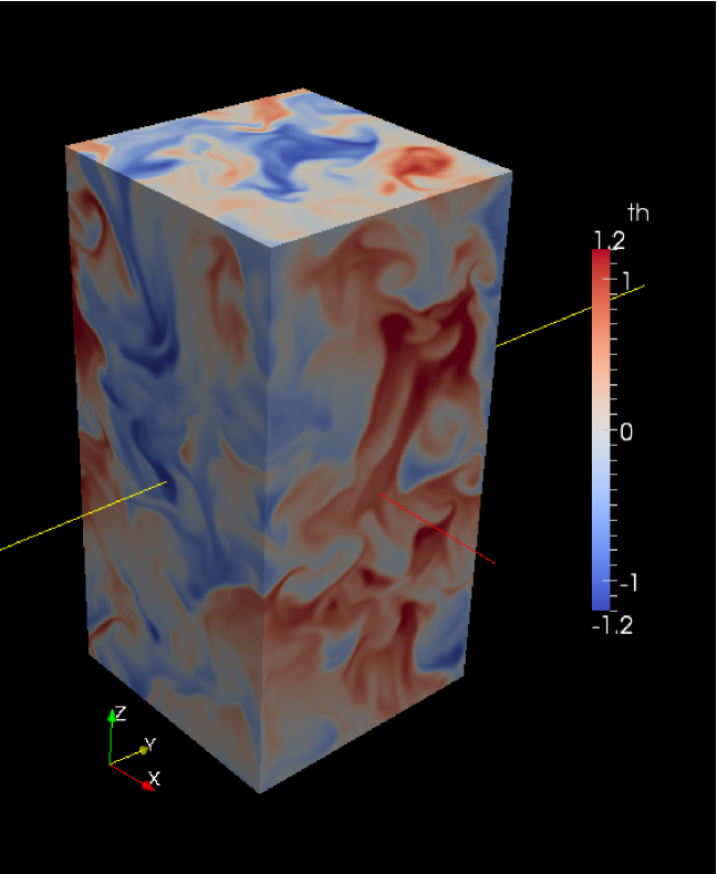
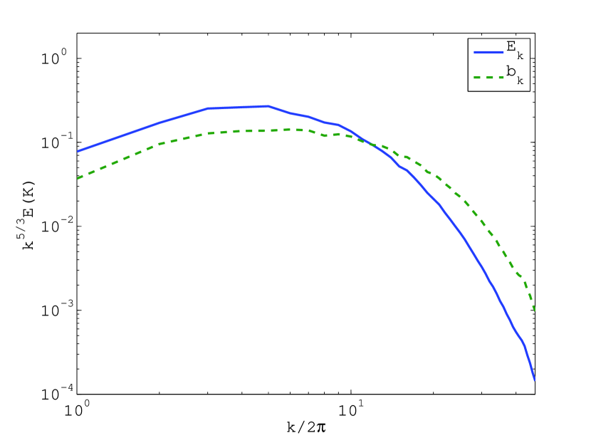
Figure 1: Simulation snapshot of thermal fluctuations (top) and energy spectra (bottom) at $Ra=4\times 10^{6}$ in the case without any shear. We show the kinetic energy spectrum ($E_{k}$) and the temperature fluctuation spectrum ($b_{k}$).

4.2 Turbulent viscosity: definitions and simple models

Traditionally, the turbulent viscosity is associated with a simple closure formula relating the Reynolds stress to the rate of strain; in our system,

$$-R_{xy}=\nu_{\mathrm{t}}\dot{a}.$$ (56)

This expression is based on the assumptions that the relationship between stress and rate of strain is linear and instantaneous. In the case of rapid oscillatory shear, the assumption of linearity is reasonable provided that the shear is of sufficiently small amplitude. However, the assumption of instantaneity is generally not valid and we should allow the Reynolds stress to be linearly related to $\dot{a}(t)$ through an integral over its previous history. In the Fourier domain, this relationship (a convolution) reduces to a multiplication:

$$-\widetilde{R}_{xy}(\omega)=\nu_{\mathrm{t}}(\omega)\widetilde{\dot{a}}(\omega),$$ (57)

where $\widetilde{\cdot}$ denotes the Fourier transform in time. In this expression $\nu_{\mathrm{t}}(\omega)$ is a complex function of frequency, rather than a real constant, indicating that the Reynolds stress and the rate of strain are generally out of phase, and that the relationship is frequency-dependent. Since the relationship involves real-valued functions in the temporal domain, $\nu_{\mathrm{t}}$ has the Hermitian symmetry $\nu_{\mathrm{t}}(-\omega)=[\nu_{\mathrm{t}}(\omega)]^{*}$ for real $\omega$. With our choice of $\dot{a}=-S\cos(\Omega t)$, we have

$$\widetilde{R}_{xy}(\omega)=\nu_{\mathrm{t}}(\omega)S\,\pi[\delta(\omega-\Omega)+\delta(\omega+\Omega)].$$ (58)

This makes it possible to measure $\nu_{\mathrm{t}}(\Omega)$ from the time series $R_{xy}(t)$. In reality, the delta function is replaced by a peak of finite height and non-zero width because of the finite integration time; alternatively, it becomes a Kronecker delta in a discrete Fourier transform. Furthermore, noise is present because there are turbulent fluctuations in $R_{xy}$ even in the absence of shear. The integration time must be sufficiently long to allow the signal to be detected above the noise.

A simple closure model for the Reynolds stress that can be compared with the results of numerical simulations is a viscoelastic model, which reflects the fact that the turbulent stress cannot instantaneously produce a viscous response to a time-dependent shear rate. [Viscoelastic models for magnetohydrodynamic turbulence in astrophysical discs have been discussed by Ogilvie (2001).] We suppose that the convective turbulence contains a number of viscoelastic components, having effective elastic moduli $c_{j}$ and relaxation times $1/\gamma_{j}$, giving rise to the complex turbulent viscosity

$$\nu_{\mathrm{t}}(\omega)=\sum_{j}\frac{c_{j}}{\gamma_{j}-\mathrm{i}\omega}.$$ (59)

In this expression, $c_{j}$ and $\gamma_{j}$ are real, but we do not require $c_{j}>0$, allowing for the possibility that negative $\mathrm{Re}[\nu_{\mathrm{t}}(\omega)]$ may appear for some ranges of frequency. For example, the case of constant shear rate ($\omega=0$) is known to produce negative viscosity for low values of $Ra$ in protoplanetary disc convection, which involves rotation as well as shear (Lesur & Ogilvie, 2010). However, in order to have a physical relaxation for all possible input signals, we require $\gamma_{j}>0$, indicating that the system we describe is stable for any time-dependent shear. In other words, since $\nu_{\mathrm{t}}(\omega)$ in equation (57) derives from a causal integral relationship, it should be analytic in the upper half-plane.

This model shares several properties with the analytical results derived in Section 3. In the high-frequency limit $\omega\to\infty$, the model gives

$$\nu_{t}=\mathrm{i}\omega^{-1}\sum_{j}c_{j}+\omega^{-2}\sum_{j}c_{j}\gamma_{j}+O(\omega^{-3}).$$ (60)

This behaviour is equivalent to equation (42) obtained for the high-frequency response of an arbitrary flow, if $\mathcal{G}_{0}=\sum_{j}c_{j}$ (the high-frequency elastic modulus) and $\mathcal{G}_{1}=\sum_{j}c_{j}\gamma_{j}$. (On the other hand, the viscosity obtained in the low-frequency limit $\omega\to 0$ is $\sum_{j}c_{j}/\gamma_{j}$.) As we will see later, the same type of dependency is found in numerical simulations.

In this paper, we will assume that only two viscoelastic components are present. This can be seen as a computational limitation, since numerical simulations cannot probe very high frequencies which are usually associated with scales below the grid size. In the following, we will therefore consider the simplified model

$$\nu_{\mathrm{t}}(\omega)=\frac{c_{1}}{\gamma_{1}-\mathrm{i}\omega}+\frac{c_{2}}{\gamma_{2}-\mathrm{i}\omega}.$$ (61)

4.3 Measuring the turbulent viscosity

A typical example of the time series of the Reynolds stress and its Fourier transform are shown in Fig. 2. In order to reduce the aliasing of low frequencies into the high-frequency domain due to the finite integration time, we have applied a Hanning window to the time series before computing the Fourier transform. As is evident from the time series, the turbulent convection produces large fluctuations in the Reynolds stress which dominate the response to the oscillatory shear. Nevertheless, it is possible to extract useful information by looking at the temporal spectrum of the stress. In particular, a spike is clearly visible at $\omega=\Omega$, which indicates that the turbulent flow is producing a detectable response to our forcing. With the complete Fourier transform of the Reynolds stress, it is possible to measure the turbulent viscosity at the forcing frequency using equation (58). Moreover, evaluating the noise level in the vicinity of the spike allows us to estimate the uncertainty in the measurement of the turbulent viscosity.

It should be noted that the signal-to-noise ratio (defined as the ratio of the amplitude of the spectral spike to the amplitude of the surrounding noise; see Fig. 2, right panel) should decay as $\Delta T^{-1/2}$. Therefore, if the oscillatory signal (the spectral spike) is too weak to be detected in the Fourier transform, one can in principle increase the integration time to reduce the signal-to-noise ratio, but this is a computationally expensive procedure.

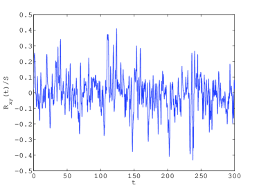
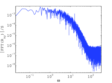
Figure 2: Time history of the Reynolds stress (left) and Fourier transform of the Reynolds stress (right) with an oscillatory shear of frequency $\Omega=16$ and amplitude $S=0.1$. The periodic signal cannot be seen in the time series. The Fourier transform exhibits a peak at the excitation frequency $\omega=\Omega$.

4.4 Numerical results

The results of the simulations performed in this work are shown in Table 1. They are also plotted in Fig. 3 for shearwise convection and in Fig. 4 for spanwise convection. Despite the present of significant noise in some of the results, several deductions can be made from these simulations:

$Ra$	$\bm{e}$ direction	$\Delta T$	$\Omega$	$S$	$K$	$\mathrm{Re}(\nu_{\mathrm{t}})$	$\mathrm{Im}(\nu_{\mathrm{t}})$	error
$4\times 10^{6}$	$x$	500	0.25	0.1	$2.1\times 10^{-1}$	$7.9\times 10^{-2}$	$2.7\times 10^{-2}$	$1.2\times 10^{-2}$
$4\times 10^{6}$	$x$	300	0.5	0.1	$2.2\times 10^{-1}$	$6.8\times 10^{-2}$	$3.4\times 10^{-2}$	$3.0\times 10^{-2}$
$4\times 10^{6}$	$x$	300	1.0	0.1	$2.1\times 10^{-1}$	$4.5\times 10^{-2}$	$4.1\times 10^{-2}$	$2.2\times 10^{-2}$
$4\times 10^{6}$	$x$	300	2.0	0.1	$2.2\times 10^{-1}$	$2.1\times 10^{-2}$	$3.2\times 10^{-2}$	$1.3\times 10^{-2}$
$4\times 10^{6}$	$x$	300	4.0	0.1	$2.1\times 10^{-1}$	$3.1\times 10^{-3}$	$1.6\times 10^{-2}$	$5.2\times 10^{-3}$
$4\times 10^{6}$	$x$	300	8.0	0.1	$2.2\times 10^{-1}$	$-1.2\times 10^{-4}$	$8.6\times 10^{-3}$	$2.1\times 10^{-3}$
$4\times 10^{6}$	$x$	300	16.0	0.1	$2.2\times 10^{-1}$	$-5.6\times 10^{-5}$	$3.4\times 10^{-3}$	$3.6\times 10^{-4}$
$4\times 10^{6}$	$x$	300	32.0	0.1	$2.2\times 10^{-1}$	$-7.2\times 10^{-5}$	$1.9\times 10^{-3}$	$4.5\times 10^{-5}$
$4\times 10^{6}$	$x$	300	64.0	0.1	$2.2\times 10^{-1}$	$-1.7\times 10^{-5}$	$9.7\times 10^{-4}$	$4.0\times 10^{-6}$
$4\times 10^{6}$	$z$	300	1.0	0.1	$2.3\times 10^{-1}$	$1.7\times 10^{-2}$	$1.6\times 10^{-2}$	$5.6\times 10^{-3}$
$4\times 10^{6}$	$z$	300	2.0	0.1	$2.1\times 10^{-1}$	$1.4\times 10^{-2}$	$1.3\times 10^{-2}$	$4.6\times 10^{-3}$
$4\times 10^{6}$	$z$	300	4.0	0.1	$2.2\times 10^{-1}$	$6.3\times 10^{-3}$	$1.3\times 10^{-2}$	$3.4\times 10^{-3}$
$4\times 10^{6}$	$z$	300	8.0	0.1	$2.2\times 10^{-1}$	$-6.5\times 10^{-4}$	$5.7\times 10^{-3}$	$1.4\times 10^{-3}$
$4\times 10^{6}$	$z$	300	16.0	0.1	$2.2\times 10^{-1}$	$-1.6\times 10^{-4}$	$2.8\times 10^{-3}$	$4.0\times 10^{-4}$
$4\times 10^{6}$	$z$	700	0.25	0.05	$2.2\times 10^{-1}$	$2.3\times 10^{-2}$	$8.8\times 10^{-3}$	$8.9\times 10^{-3}$
$4\times 10^{6}$	$z$	700	0.5	0.05	$2.2\times 10^{-1}$	$2.1\times 10^{-2}$	$6.8\times 10^{-3}$	$9.4\times 10^{-3}$
$4\times 10^{6}$	$z$	600	1.0	0.05	$2.2\times 10^{-1}$	$1.0\times 10^{-2}$	$1.9\times 10^{-2}$	$8.4\times 10^{-3}$
$4\times 10^{6}$	$z$	600	2.0	0.05	$2.2\times 10^{-1}$	$8.9\times 10^{-3}$	$1.3\times 10^{-2}$	$7.2\times 10^{-3}$
$4\times 10^{6}$	$z$	600	4.0	0.05	$2.2\times 10^{-1}$	$4.2\times 10^{-3}$	$9.6\times 10^{-3}$	$4.0\times 10^{-3}$
$4\times 10^{6}$	$z$	300	8.0	0.05	$2.2\times 10^{-1}$	$1.3\times 10^{-3}$	$5.8\times 10^{-3}$	$2.9\times 10^{-3}$
$4\times 10^{6}$	$z$	300	16.0	0.05	$2.1\times 10^{-1}$	$-1.7\times 10^{-4}$	$2.4\times 10^{-3}$	$6.7\times 10^{-4}$
$4\times 10^{6}$	$z$	300	32.0	0.05	$2.2\times 10^{-1}$	$-8.0\times 10^{-5}$	$1.3\times 10^{-3}$	$9.0\times 10^{-5}$
$4\times 10^{6}$	$z$	300	64.0	0.05	$2.2\times 10^{-1}$	$-4.0\times 10^{-6}$	$6.2\times 10^{-4}$	$6.5\times 10^{-6}$
$1\times 10^{5}$	$z$	3600	64.0	0.1	$2.6\times 10^{-1}$	$-5.7\times 10^{-6}$	$7.0\times 10^{-4}$	$3.9\times 10^{-7}$

Table 1: Parameters and results of the simulations discussed in this paper. The error in $\nu_{\mathrm{t}}$ is estimated based on the rms turbulent noise in the Fourier transform at the oscillation frequency. $K$ is the mean kinetic energy density of the fluctuations.

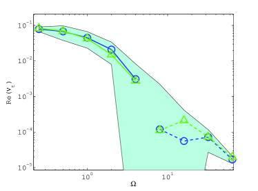
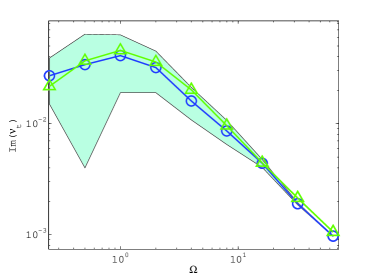
Figure 3: Turbulent viscosity of shearwise convection, versus the angular oscillation frequency in units of $|N|$. The numerical measurements are shown in blue (open circles) and the best fit of the closure model (61) is shown in green (triangles). Negative values are connected by a dashed line. Uncertainties due to turbulent noise are shown as a shaded region.

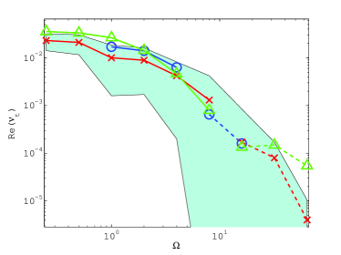
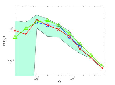
Figure 4: Turbulent viscosity of spanwise convection, versus the angular oscillation frequency in units of $|N|$. The numerical measurements are shown in blue (open circles; $S=0.1$) and red (crosses; $S=0.05$) and the best fit of the closure model (61) is shown in green (triangles). Negative values are connected by a dashed line. Uncertainties due to turbulent noise are shown as a shaded region.

• At sufficiently high frequency, we find $\mathrm{Re}(\nu_{\mathrm{t}})<0$ in every case. Note, however, that noise dominates many high-frequency measurements of this quantity. To substantiate the high-frequency behaviour, we have performed a simulation at lower Rayleigh number ($Ra=10^{5}$) for more than 3000 turnover times in order to reduce the effect of turbulent noise. This simulation exhibits clearly $\mathrm{Re}(\nu_{\mathrm{t}})<0$ at $\Omega=64$, indicating that the trend observed in the other configurations is real.

• $\mathrm{Im}(\nu_{\mathrm{t}})>0$. This conclusion is rather strong since the noise level is smaller than the measured value of $\mathrm{Im}(\nu_{\mathrm{t}})$ in most cases. It means that the effective elasticity is positive.

• Larger values of $|\nu_{\mathrm{t}}|$ are found when the stratification is in the $x$ direction (shearwise convection). This suggests that the full turbulent viscosity tensor is anisotropic.

• Changing $S$ does not change significantly the measured turbulent viscosity, suggesting that the numerical simulations are in the linear regime assumed in writing down equation (57). However, the results obtained with the smaller value of $S$ are subject to significant uncertainty.

• The asymptotic behaviour in the high-frequency limit is $\mathrm{Re}(\nu_{\mathrm{t}})\propto\omega^{-2}$ and $\mathrm{Im}(\nu_{\mathrm{t}})\propto\omega^{-1}$.

We have also fitted the simple closure model (61) to the numerical results for shearwise and spanwise convection. The best fits are shown as green curves in Figs 3 and 4, and the coefficients we obtained are shown in Table 2. The major viscoelastic component has an effective elastic modulus $c_{1}$ that is comparable to, but somewhat less than, the mean kinetic energy density $K$ (cf. eq. 46, which suggests a ratio of $4/15$ in the isotropic case) and a relaxation rate comparable to the nominal convective turnover rate $|N|$, which is $1$ in our system of units. Note that the contribution to $\mathrm{Re}(\nu_{\mathrm{t}})$ from the first component is $(c_{1}/\gamma_{1})[1+(\omega/\gamma_{1})^{2}]^{-1}$, which is compatible with the form of the frequency-dependent viscosity used by Ogilvie & Lin (2007). The suggested presence of a second viscoelastic component with a negative $c_{2}$ and a faster relaxation indicates that, at high frequency, the real part of the viscosity changes sign, as is observed in the numerical results. With more data we might be led to introduce a broader spectrum of viscoelastic components.

coefficient	shearwise convection	spanwise convection
$c_{1}$	$0.0978$	$0.06$
$\gamma_{1}$	$1.07$	$1.62$
$c_{2}$	$-0.0286$	$-0.0178$
$\gamma_{2}$	$6.15$	$24.25$

Table 2: Best-fit coefficients for the closure model (61).

In order to identify which spatial scales contribute to the turbulent viscosity, we have computed the spatial ‘spectrum’ of the turbulent viscosity. This is derived from the instantaneous spatial spectrum of the Reynolds stress,

$$\widehat{R}_{xy}(k,t)=2\,\mathrm{Re}\Big{[}\overline{\hat{v}_{x}\hat{v}_{y}^{*}}\Big{]},$$ (62)

where $\hat{v}_{i}$ is the 3D instantaneous spatial Fourier transform of $v_{i}$ and the overbar denotes a shell-integration procedure in spectral space, such that $R_{xy}(t)=\int_{0}^{\infty}\widehat{R}_{xy}(k,t)\,\mathrm{d}k$. $\hat{R}_{xy}(k,t)$ is then used in a relation similar to (58) which defines the turbulent viscosity spectrum $\widehat{\nu_{\mathrm{t}}}(k,\omega)$:

$$\widetilde{\widehat{R}}_{xy}(k,\omega)=\widehat{\nu_{\mathrm{t}}}(k,\omega)S\,\pi\big{[}\delta(\omega-\Omega)+\delta(\omega+\Omega)\big{]}.$$ (63)

We have applied this procedure to the simulation with $\Omega=16$, $S=0.1$ and with stratification in the $z$ direction. The corresponding spectra are shown in Fig. 5. As can be seen, much of the turbulent viscosity (both real and imaginary) is due to the largest scales of the system. However, we also observe a component with $\mathrm{Re}(\nu_{\mathrm{t}})>0$ at ‘small’ scales ($k/2\pi\sim 10$), indicating that there may be an important contribution from scales whose turnover time is of the order of the tidal frequency. It should be stressed that these spectra are strongly polluted by turbulent noise, especially at low wavenumbers. Therefore, this result should be seen as a plausible trend. Longer simulations having a larger resolution should be used to confirm this finding.

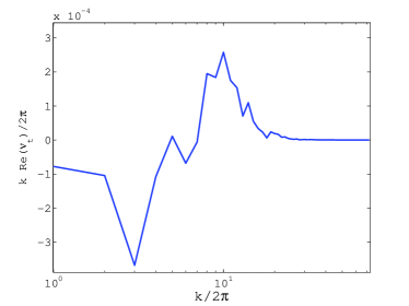
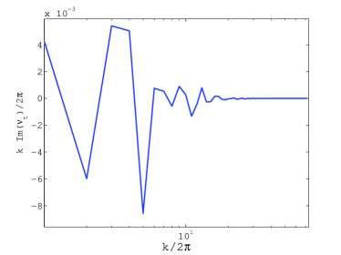
Figure 5: Spatial spectrum of the turbulent viscosity for the simulation of spanwise convection with $\Omega=16$ and $S=0.1$. The real part has two components: a negative contribution from large scales and a positive contribution from smaller scale ($k/2\pi\sim 10$).

5 Summary and discussion

In this paper we have studied the interaction between tides and convection in astrophysical bodies by analysing the effect of a homogeneous oscillatory shear on a fluid flow. This model can be taken to represent the interaction between a large-scale periodic tidal deformation and a smaller-scale convective motion. We first considered analytically the limit in which the shear is of low amplitude and the oscillation period is short compared to the timescales of the unperturbed flow. In this limit there is a viscoelastic response and we obtained expressions for the effective elastic modulus and viscosity coefficient. The effective viscosity is inversely proportional to the square of the oscillation frequency, with a coefficient that can be positive, negative or zero depending on the properties of the unperturbed flow. We also carried out direct numerical simulations of Boussinesq convection in an oscillatory shearing box and measured the time-dependent Reynolds stress. The results indicate that the effective viscosity falls rapidly as the oscillation frequency is increased, attaining small negative values in the cases we have examined.

Our methods and findings differ significantly from those of other authors. The hypothesis of Zahn (1966) that the effective viscosity of large eddies is reduced by only a linear factor at high frequencies is incompatible with our analytical and numerical results. We find a quadratic reduction factor at high frequencies, similarly to Goldreich & Nicholson (1977) and Goldreich & Keeley (1977), but not necessarily for the same reason. Our analytical study, which goes beyond that of Goodman & Oh (1997), implies that large eddies generically provide a quadratically reduced viscosity [which Goldreich & Nicholson (1977) considered as an upper bound], but with a coefficient that can be positive, negative or zero. Our numerical results also indicate a quadratically reduced viscosity, with a tendency towards negative values at high frequencies in the cases we have examined, an effect due to the largest scales in the turbulent flow.

The appearance of a negative effective viscosity may be alarming. However, there is no reason in principle why the effective viscosity of a convective fluid need be positive. The consequence of a negative effective viscosity would be that tidal evolution proceeds in the reverse direction to that usually assumed. Angular momentum would be transferred in an ‘anti-frictional’ direction, from the less rapidly rotating component to the more rapidly rotating one. For example, if a small satellite orbits a body with a negative effective viscosity, and if the larger body spins more slowly than the orbit, then the orbit would expand and the larger body would spin down. Energy would be added to the spin-orbit system. (Similarly, orbital eccentricity could be caused to increase in situations where circularization would usually be expected.) While this effect might be called tidal ‘anti-dissipation’, it does not contradict the laws of thermodynamics. Within limits, work can indeed be done by the convection on the tidal flow; the energy comes from the buoyancy forces that drive the convection, and ultimately from nuclear or gravitational energy. Since we are considering a regime in which the tidal strain is small and the tidal frequency is high (implying that the negative effective viscosity is much smaller in magnitude than the values estimated from mixing-length theory), only a very small fraction of the energy budget of the star would be diverted into the spin-orbit system. The consequences could still be important, because the nuclear energy content of the Sun, for example, is about five orders of magnitude larger than the orbital energy of (say) a solar-type binary star with an orbital period of ten days.

A well known example of a related phenomenon is the negative effective viscosity of convection at low or moderate Rayleigh number in an accretion disc (Lesur & Ogilvie, 2010, and references therein), which would lead to anti-frictional angular momentum transport and anti-diffusion of the surface density of the disc. This example also serves as a reminder that the Coriolis force present in a rotating system can affect the transport of (angular) momentum; it would therefore be of interest to include rotation in the calculations presented in this paper. Anti-frictional processes are also well known in the context of the Earth’s atmosphere (e.g. McIntyre, 2000).

There are several reasons why this reversed tidal evolution may not, in fact, be found in nature. First, it may be that when a more realistic tidal velocity field is considered and the actual anisotropies of the convection and the Coriolis force are taken into account, the net effective viscosity turns out to be positive. Second, in a solar-type star where the convective timescale becomes short near the surface, the net effective viscosity may be dominated by these more rapid convective elements and work out to be positive. Third, it may be that tidal dissipation is dominated by internal waves and that convection makes a relatively small contribution. Fourth, the negative effective viscosities that we find might be due to explicit (molecular) viscous effects which are totally negligible in astrophysical objects. Indeed, we have not found a negative turbulent viscosity that exceeds the explicit (molecular) viscosity in magnitude. Nevertheless, it is of interest to note the theoretical possibility of reversed tidal evolution and to be alert to any observational evidence of such an effect.

Penev and collaborators have attempted to address the issue of the reduction of the effective viscosity at high frequencies through simulations of convection in a deep layer. While their results suggest only a linear reduction factor (and a positive numerical value), there are many differences between their work and ours. Our numerical study involves a local model of convection, which is in some ways more limited but is also more controlled because a uniform unstable stratification is imposed. We measure the effective viscosity directly rather than relying on a perturbative calculation or an indirect measurement. Penev et al. (2009) do not find good agreement between different methods, and their results depend on the shear amplitude. Our work covers a wider range of oscillation frequencies and quantifies the uncertainty due to turbulent noise. It should also be pointed out that our work uses a very small forcing compared to Penev and collaborators. In particular, the rms velocities with and without forcing are identical in all our runs, whereas Penev et al. (2009) have forced velocities of the order of the rms velocity in their case of weak forcing, and even 5 times larger in the case of strong forcing. We believe that such strong forcing could significantly affect the measurement of turbulent viscosity. Several tests that we have performed indicate that doubling the forcing amplitude (to $S=0.2$) is already enough to modify our results.

In our opinion more work is required to extend both analytical and numerical calculations of this type before the frequency-dependent effective viscosity of a realistic stellar or planetary convective zone can be reliably estimated, and the efficiency of tidal dissipation in astrophysical bodies can be better understood.

Appendix A Composition of an arbitrary traceless velocity gradient tensor from simple shears

We consider an arbitrary incompressible velocity gradient tensor, being a $3\times 3$ matrix with vanishing trace. Each of the off-diagonal elements represents a simple shear, and therefore the off-diagonal part of the matrix is a linear combination of simple shears. To compose the diagonal elements, we first consider the matrix

$$\left(\begin{matrix}0&1&0\\ 1&0&0\\ 0&0&0\end{matrix}\right),$$ (64)

which is a linear combination of simple shears. By a rotation through $\pi/4$ about the $z$ axis, we bring this matrix into the diagonal form

$$\left(\begin{matrix}1&0&0\\ 0&-1&0\\ 0&0&0\end{matrix}\right).$$ (65)

In a similar way the matrix

$$\left(\begin{matrix}1&0&0\\ 0&0&0\\ 0&0&-1\end{matrix}\right)$$ (66)

can be constructed from simple shears. Using a linear combination of these two diagonal matrices, the three diagonal elements of the arbitrary velocity gradient tensor can be composed, subject to the constraint that the sum of the diagonal elements vanishes.

Appendix B Vanishing of certain triple velocity correlations for statistically isotropic flows

Let ${\mn@boldsymbol{v}}({\mn@boldsymbol{x}})$ be a solenoidal vector field in $d\geq 2$ dimensions satisfying periodic boundary conditions, and let $\langle\cdot\rangle$ be a spatial average over a periodic cell. (We omit primes on ${\mn@boldsymbol{x}}$ and ${\mn@boldsymbol{\nabla}}$ in this Appendix.) We assume that ${\mn@boldsymbol{v}}({\mn@boldsymbol{x}})$ has zero mean and is statistically isotropic so that any averages of tensor products of ${\mn@boldsymbol{v}}$ and its derivatives are isotropic tensors. The inverse Laplacian operator $\Delta^{-1}$ is well defined and self-adjoint for periodic fields of zero mean.

We first consider the tensor

$$D_{abcd}=\langle v_{a}v_{b}\partial_{c}v_{d}\rangle.$$ (67)

As an isotropic tensor, this must be a linear combination of products of Kronecker deltas:

$$D_{abcd}=t_{1}\delta_{ab}\delta_{cd}+t_{2}\delta_{ac}\delta_{bd}+t_{3}\delta_{ad}\delta_{bc}.$$ (68)

The symmetry and contraction conditions $D_{abcd}=D_{bacd}$ and $D_{abcc}=0$ imply $t_{2}=t_{3}$ and $dt_{1}+t_{2}+t_{3}=0$. Thus

$$D_{abcd}=t_{4}[d(\delta_{ac}\delta_{bd}+\delta_{ad}\delta_{bc})-2\delta_{ab}\delta_{cd}].$$ (69)

However, we also have

$$D_{abba}=\langle v_{a}v_{b}\partial_{b}v_{a}\rangle=\langle\partial_{b}({\textstyle\frac{1}{2}}v_{a}v_{a}v_{b})\rangle=0=t_{4}d(d-1)(d+2),$$ (70)

and so

$$D_{abcd}=0.$$ (71)

We next consider

$$D_{abcdef}=\langle v_{a}v_{b}\partial_{c}\partial_{d}\partial_{e}\Delta^{-1}v_{f}\rangle.$$ (72)

Isotropy and symmetry imply

$$\begin{split}&D_{abcdef}=t_{5}(\delta_{ab}\delta_{cd}\delta_{ef}+\delta_{ab}\delta_{ce}\delta_{df}+\delta_{ab}\delta_{cf}\delta_{de})\\ &\qquad+t_{6}(\delta_{ac}\delta_{bd}\delta_{ef}+\delta_{ac}\delta_{be}\delta_{df}+\delta_{ad}\delta_{bc}\delta_{ef}+\delta_{ad}\delta_{be}\delta_{cf}+\delta_{ae}\delta_{bc}\delta_{df}+\delta_{ae}\delta_{bd}\delta_{cf})\\ &\qquad+t_{7}(\delta_{ac}\delta_{bf}\delta_{de}+\delta_{ad}\delta_{bf}\delta_{ce}+\delta_{ae}\delta_{bf}\delta_{cd}+\delta_{af}\delta_{bc}\delta_{de}+\delta_{af}\delta_{bd}\delta_{ce}+\delta_{af}\delta_{be}\delta_{cd}).\end{split}$$

(There are three types of term here: those in which the two undifferentiated $v$s are paired, those in which each such $v$ is paired with a $\partial$, and those in which one of them is paired with the differentiated $v$. Symmetry demands that the coefficients of terms of the same type are equal.)

We require the contraction $D_{abcdee}$ (and those related by symmetry) to vanish. Thus

$$(d+2)t_{5}\delta_{ab}\delta_{cd}+t_{6}(d+2)(\delta_{ac}\delta_{bd}+\delta_{ad}\delta_{bc})+2t_{7}(\delta_{ab}\delta_{cd}+\delta_{ac}\delta_{bd}+\delta_{ad}\delta_{bc})=0,$$ (73)

which implies $t_{5}=t_{6}$ and $(d+2)t_{5}=-2t_{7}$, and so

$$\begin{split}&D_{abcdef}=t_{8}[(d+2)(\delta_{ac}\delta_{bf}\delta_{de}+\delta_{ad}\delta_{bf}\delta_{ce}+\delta_{ae}\delta_{bf}\delta_{cd}+\delta_{af}\delta_{bc}\delta_{de}+\delta_{af}\delta_{bd}\delta_{ce}+\delta_{af}\delta_{be}\delta_{cd})\\ &\qquad-2(\delta_{ab}\delta_{cd}\delta_{ef}+\delta_{ab}\delta_{ce}\delta_{df}+\delta_{ab}\delta_{cf}\delta_{de}+\delta_{ac}\delta_{bd}\delta_{ef}+\delta_{ac}\delta_{be}\delta_{df}+\delta_{ad}\delta_{bc}\delta_{ef}+\delta_{ad}\delta_{be}\delta_{cf}+\delta_{ae}\delta_{bc}\delta_{df}+\delta_{ae}\delta_{bd}\delta_{cf})].\end{split}$$

The contraction $D_{abcddf}$ (and those related by symmetry) produces a Laplacian, so $D_{abcddf}=D_{abcf}$, which we have already shown to vanish. Thus

$$(d+4)t_{8}[d(\delta_{ac}\delta_{bf}+\delta_{af}\delta_{bc})-2\delta_{ab}\delta_{cf}]=0,$$ (74)

which implies $t_{8}=0$ and so

$$D_{abcdef}=0.$$ (75)

The last tensor to consider is

$$D_{abcdefgh}=\langle v_{a}v_{b}\partial_{c}\partial_{d}\partial_{e}\partial_{f}\partial_{g}\Delta^{-2}v_{h}\rangle.$$ (76)

We give an abbreviated argument. Isotropy and symmetry imply

$$\begin{split}&D_{abcdefgh}=t_{9}(\delta_{ab}\delta_{cd}\delta_{ef}\delta_{gh}+\delta_{ab}\delta_{cd}\delta_{eg}\delta_{fh}+\cdots)+t_{10}(\delta_{ac}\delta_{bd}\delta_{ef}\delta_{gh}+\delta_{ac}\delta_{bd}\delta_{eh}\delta_{fg}+\cdots)\\ &\qquad+t_{11}(\delta_{ah}\delta_{bc}\delta_{df}\delta_{eg}+\delta_{ah}\delta_{bc}\delta_{dg}\delta_{ef}+\cdots).\end{split}$$

Requiring the contraction $D_{abcdefgg}$ to vanish implies $t_{9}=t_{10}$ and $(d+4)t_{9}=-t_{11}$. The contraction $D_{abccefgh}$ should produce $D_{abefgh}$, which we have already shown to vanish. This is of the form given above, with $t_{5}=(d+4)t_{9}+2t_{10}$, $t_{6}=(d+6)t_{10}$ and $t_{7}=2t_{10}+(d+4)t_{11}$. Therefore $t_{9}=t_{10}=t_{11}=0$ and so $D_{abcdefgh}=0$.

References

- Arnol’d (1965) Arnol’d V. I., 1965, C. R. Acad. Sci. Paris, 261, 17
- Darwin (1880) Darwin G. H., 1880, Phil. Trans. R. Soc. London, 171, 713
- Galloway & Frisch (1987) Galloway D., Frisch U., 1987, JFM, 180, 557
- Goldreich & Keeley (1977) Goldreich P., Keeley D. A., 1977, ApJ, 211, 934
- Goldreich & Nicholson (1977) Goldreich P., Nicholson P. D., 1977, Icar, 30, 301
- Goodman & Oh (1997) Goodman J., Oh S. P., 1997, ApJ, 486, 403
- Hawley, Gammie & Balbus (1995) Hawley J. F., Gammie C. F., Balbus S. A., 1995, ApJ, 440, 742
- Lesur & Longaretti (2005) Lesur G., Longaretti P.-Y., 2005, A&A, 444, 25
- Lesur & Longaretti (2007) Lesur G., Longaretti P.-Y., 2007, MNRAS, 378, 1471
- Lesur & Ogilvie (2010) Lesur G., Ogilvie G. I., 2010, MNRAS, 404, L64
- McIntyre (2000) McIntyre M. E., 2000, in Batchelor, G. K, Moffatt, H. K., Worster, M. G., eds, Perspectives in Fluid Dynamics, Cambridge Univ. Press, 557
- Meibom & Mathieu (2005) Meibom S., Mathieu R. D., 2005, ApJ, 620, 970
- Ogilvie (2001) Ogilvie G. I., 2001, MNRAS, 325, 231
- Ogilvie & Lin (2004) Ogilvie G. I., Lin D. N. C., 2004, ApJ, 610, 477
- Ogilvie & Lin (2007) Ogilvie G. I., Lin D. N. C., 2007, ApJ, 661, 1180
- Penev, Barranco & Sasselov (2009) Penev K., Barranco J., Sasselov D., 2009, ApJ, 705, 285
- Penev et al. (2009) Penev K., Sasselov D., Robinson F., Demarque P., 2009, ApJ, 704, 930
- Penev et al. (2007) Penev K., Sasselov D., Robinson F., Demarque P., 2007, ApJ, 655, 1166
- Rogallo (1981) Rogallo R. S., 1981, NASA Technical Memorandum 81315
- Wirth, Gama & Frisch (1995) Wirth A., Gama S., Frisch U., 1995, JFM, 288, 249
- Wisdom & Tremaine (1988) Wisdom J., Tremaine S., 1988, AJ, 95, 925
- Zahn (1966) Zahn J. P., 1966, AnAp, 29, 489