Abstract

The $\beta$-deformation is one of the two superconformal deformations of the ${\cal N}=4$ super-Yang-Mills theory. At the planar level it shares all of its properties except for supersymmetry, which is broken to the minimal amount. The tree-level amplitudes of this theory exhibit new features which depart from the commonly assumed properties of gauge theories with fields in the adjoint representation.

We analyze in detail complete one-amplitudes and a nonplanar two-loop amplitude of this theory and show that, despite having only ${\cal N}=1$ supersymmetry, the two-loop amplitudes have a further-improved ultraviolet behavior. This phenomenon is a counterpart of a similar improvement previously observed in the double-trace amplitude of the ${\cal N}=4$ super-Yang-Mills theory at three and four loop order and points to the existence of additional structure in both the deformed and undeformed theories.

1 Introduction

The maximally supersymmetric Yang-Mills (sYM) theory has provided a valuable arena for devising new and powerful methods for perturbative quantum field theory computations. In the planar limit, this effort exposed remarkable properties of the theory, such as dual (super)conformal invariance and integrability, as well as unexpected relations between a priori unrelated quantities, such as the relation between certain null polygonal Wilson loops, scattering amplitudes and correlation functions of gauge invariant operators. Each of these presentations of scattering amplitudes, as a Wilson loop or as a (square root of a) correlation function, manifestly realizes one of the two conformal symmetries of the theory. It has been suggested that, in four dimensions, the symmetries of the theory together with the leading singularities of amplitudes completely determine the planar loop integrand to all orders in perturbation theory [1].

At the nonplanar level the symmetry structure of the theory is expected to be different. While comparatively less studied, explicit calculations of complete amplitudes [2, 3] expose unexpected structure: the color/kinematics duality and the BCJ relations [4], generalizing the $U(1)$ decoupling identities and the Kleiss-Kuijff relations, provide a direct link between the planar and non-planar parts of amplitudes. They also suggest that the kinematic numerators of integrands of amplitudes (once organized in a specific way) obey an algebra akin to that of the color factors. The fundamental origin as well as its implications and limitations are not completely understood (see however [5] for an interesting discussion in the self-dual sector). The color/kinematic duality has also been discussed in less supersymmetric theories [4].

A possible strategy to identify the essential elements underlying the fascinating properties of the ${\cal N}=4$ sYM theory at the non-planar level is to deform this theory in a way that does not alter its planar properties and then analyze the resulting theory. Since such deformations necessarily break supersymmetry, this analysis would also probe, in a more general context, other aspects of the undeformed theory: the possibility and subtleties associated to using the Coulomb branch as infrared regulator even at the planar level; the consistency conditions on massless S-matrices discussed in [6], etc. A further appeal of this strategy is that, by reducing the number of supercharges, unexpected phenomena unrelated to maximal supersymmetry but hidden by it may emerge at low loop order.

The two deformations of the ${\cal N}=4$ sYM theory which preserve conformal invariance to all orders in perturbation theory at both planar and non-planar level have been identified by Leigh and Strassler in [7]. In both cases the arguments described there show that there exists a relation between the gauge coupling, the strength of the deformation and the number of colors which, if satisfied, guarantees conformal invariance of the theory.

The so-called $\beta$-deformation was extensively studied from several standpoints. The planar scattering amplitudes have been discussed in [8] where it was shown that, for real $\beta$, they are inherited from the undeformed theory and thus are dual conformally invariant. From the current perspective this result reinforces the link between integrability and dual conformal invariance. Indeed, the $\beta$-deformation preserves integrability both at weak [9] and strong coupling [10] and the construction of its string theory dual [11, 10] suggests that the arguments of [12, 13] relating integrability and dual conformal symmetry should apply in this case as well.

While the existence of a line of fixed points is guaranteed by the arguments of [7], the precise relation between parameters is known in general only through two-loop order. Our calculations of four-point amplitudes at one- and two-loop level will confirm the known constraint. We will argue that this constraint must be modified at three loops. This is similar in spirit to the argument of [8] that, for complex deformation parameter, the planar relation between the deformed theory and ${\cal N}=4$ sYM theory breaks down at five loops.

As all massless theories, the $\beta$-deformed ${\cal N}=4$ sYM theory has infrared divergences and therefore requires regularization. While in gauge theories IR divergences are conventionally dimensionally regulated, several possible IR regularizations are available. In the planar undeformed theory it has been argued [14] that moving off the origin of the Coulomb branch and partly breaking the gauge symmetry as $SU(N+M)\mapsto SU(N)\times SU(M)$ will on the one hand regularize IR divergences while on the other will preserve dual conformal symmetry if masses of fields (or vacuum expectation values of scalars) are assigned suitable transformation rules. An essential ingredient in these arguments is that, as a consequence of extended supersymmetry, the relation between vacuum expectation values and field masses does not receive quantum corrections. The minimal supersymmetry of the $\beta$-deformed theory does not guarantee the absence of such corrections which, as we will see, appear at the very least due to the corrections to the conformality condition. Therefore, using the Higgs regularization in the $\beta$-deformed theory at higher loops requires a certain amount of care as one should isolate the quantum corrections to the regulator. For the same reason, the close relation between the ${\cal N}=4$ and the $\beta$-deformed planar amplitudes [8], while present in dimensional regularization, does not appear to hold in a straightforward way in the Higgs regularization.

By completely breaking the gauge symmetry, $SU(N)\rightarrow U(1)^{N-1}$, the Higgs regularization may also be used at nonplanar level both in the $\beta$-deformed and in the undeformed theory. While we will draw information on the structure of amplitudes in the presence of such a regulator, we will carry out calculations in dimensional regularization. It is interesting to note that, unlike in the ${\cal N}=4$ theory, dimensional regularization changes the total number of degrees of freedom of the theory. Indeed, as an ${\cal N}=1$ theory that does not have an ${\cal N}=2$ extension, IR dimensional regularization will dimensionally-continue vector multiplets without reducing the number of chiral multiplets. For this reason the notion of critical dimension as the dimension in which the first logarithmic divergence appears at some fixed loop order is not a well-defined concept in the $\beta$-deformed theory. One may nevertheless formally continue to arbitrary dimension the integrand of an amplitude and thus define a quantity which, as we will see, captures the convergence properties of the integrand and (discontinuously) becomes the standard critical dimension as the deformation parameter is set to zero.

We will begin in the next section with a brief review of the $\beta$-deformed sYM theory, discuss its Coulomb branch and outline the main differences between its scattering amplitudes and those of the undeformed theory. In § 3 we will discuss the general features of loop calculations in this theory through the generalized unitarity method, the constraints imposed by supersymmetry and describe non-planar all-loop results that are inherited from the undeformed theory. In § 4 we present the explicit expressions for representatives of the five different classes of four-point amplitudes and discuss the properties of their infrared divergences. In § 5 we describe the first nontrivial two-loop amplitude which is sensitive to the deformation parameter and analyze its properties. We will see that, unlike the one-loop amplitudes which exhibit the standard properties of a finite ${\cal N}=1$ theory, the two-loop amplitudes we evaluate have better UV convergence properties than one might expect based on ${\cal N}=1$ supersymmetry alone. We summarize our results in § 7 and speculate on the relation of the improved UV behavior and the undeformed theory.

2 The $\beta$-deformed ${\cal N}=4$ sYM theory and its features

The $\beta$-deformed $\mathcal{N}$=4 theory is one of the two ${\cal N}=1$ exactly marginal deformations of the maximally supersymmetric Yang-Mills theory in four dimensions [7]; it is obtained by adding to the superpotential of the ${\cal N}=4$ sYM theory the term ${\delta W}={\rm Tr}[\Phi^{1}\{\Phi^{2},\Phi^{3}\}]$. The action may be written in $\mathcal{N}$=1 superspace as

$$S = \int d^{4}xd^{4}\theta\,{\rm Tr}[e^{-g_{{}_{YM}}V}\bar{\Phi}_{i}e^{g_{{}_{YM}}V}\Phi^{i}]$$

$$+ \frac{1}{2g_{{}_{YM}}^{2}}\int d^{4}xd^{2}\theta{\rm Tr}[W^{\alpha}W_{\alpha}]+ih\int d^{4}xd^{2}\theta\,{\rm Tr}[q\Phi^{1}\Phi^{2}\Phi^{3}-q^{-1}\Phi^{1}\Phi^{3}\Phi^{2}]+{\rm h.c.}\ .$$

This superspace, inherited from the one used for the ${\cal N}=4$ theory, manifestly preserves the fourth component of the ${\cal N}=4$ quartet of supercharges. The parameter $q$ is customarily parametrized as $q=\exp(i\beta)$ with $\beta$ being either real or complex. The two choices have distinct quantum mechanical properties with only the former theory, with $\beta\in\mathbb{R}$, being integrable at the planar level. In the following we will assume that $\beta$ is real.

It has been pointed out in [11] that the addition of $\delta W$ may be interpreted as a noncommutative deformation of ${\cal N}=4$ sYM theory in the R-symmetry directions; instead of space-time momenta, the relevant Moyal-like product involves the three $U(1)$ charges ${\rm q}=({\rm q}_{1},{\rm q}_{2},{\rm q}_{3})$ inherited from the $SU(4)$ symmetry of ${\cal N}=4$ sYM theory:

$$\Phi^{i}\Phi^{j}\mapsto e^{i\epsilon^{abc}\beta_{a}{\rm q}^{i}_{b}{\rm q}^{j}_{c}}\Phi^{i}\Phi^{j}\equiv e^{i\beta^{bc}{\rm q}^{i}_{b}{\rm q}^{j}_{c}}\Phi^{i}\Phi^{j}\equiv e^{i{\rm q}^{i}\wedge{\rm q}^{j}}\Phi^{i}\Phi^{j}\ ,$$ (2)

where $\beta_{1}=\beta_{2}=\beta_{3}=\beta$. It is not difficult to see that such a phase becomes trivial whenever at least one of the two fields belongs to the ${\cal N}=1$ vector multiplet. In the following we will denote by $[\bullet,\bullet]_{\beta}$ the commutator in which the product of the two entries has been replaced by the Moyal product (2), i.e.

$$[A,B]_{\beta}=e^{i\beta^{bc}{\rm q}^{A}_{b}{\rm q}^{A}_{c}}AB-e^{i\beta^{bc}{\rm q}^{B}_{b}{\rm q}^{A}_{c}}BA\ .$$ (3)

The action (2) exhibits three global U(1) symmetries. One of them is the $U(1)$ R-symmetry of the ${\cal N}=1$ superspace. The other two simultaneously rephase two of the three chiral superfields as:

$$(\Phi^{1},\Phi^{2},\Phi^{3})\mapsto(\Phi^{1},e^{i\alpha_{1}}\Phi^{2},e^{-i\alpha_{1}}\Phi^{3})\qquad(\Phi^{1},\Phi^{2},\Phi^{3})\mapsto(e^{i\alpha_{2}}\Phi^{1},e^{-i\alpha_{2}}\Phi^{2},\Phi^{3})\ .$$ (4)

Three linear combinations of these symmetries form the Cartan subalgebra of the $SU(4)$ R-symmetry of ${\cal N}=4$ sYM theory under which fermions transform in the fundamental representation (spinor representation of $SO(6)$) with charges

$${\rm q}^{1}=({\textstyle{\frac{1}{2}}},-{\textstyle{\frac{1}{2}}},-{\textstyle{\frac{1}{2}}})~{},~{}~{}{\rm q}^{2}=(-{\textstyle{\frac{1}{2}}},{\textstyle{\frac{1}{2}}},-{\textstyle{\frac{1}{2}}})~{},~{}~{}{\rm q}^{3}=(-{\textstyle{\frac{1}{2}}},-{\textstyle{\frac{1}{2}}},{\textstyle{\frac{1}{2}}})~{},~{}~{}{\rm q}^{4}=({\textstyle{\frac{1}{2}}},{\textstyle{\frac{1}{2}}},{\textstyle{\frac{1}{2}}})\ ;$$ (5)

the index $"4"$ labels the supercharges preserved by the ${\cal N}=1$ superspace in eq. (2). The scalar fields transform in the two-index antisymmetric representation (vector representation of $SO(6)$) and thus their charges may be obtained in terms of those of fermions as

$$\phi^{ij}\ ,~{}~{}{\rm q}^{ij}={\rm q}^{i}+{\rm q}^{j}\quad,\qquad\phi^{k4}\equiv{\overline{\phi^{ij}}}\ ,~{}~{}{\rm q}^{k4}={\rm q}^{k}+{\rm q}^{4}=-{\rm q}^{i}-{\rm q}^{j}~{},~{}~{}i,j,k=1,2,3\ .$$ (6)

This is the same labeling used in the ${\cal N}=4$ on-shell superspace. The phase associated to a product of fields with charges ${\rm q}_{1},\dots,{\rm q}_{n}$ is just

$$\phi_{1}\dots\phi_{n}\mapsto e^{i\varphi({\rm q}(\phi_{1}),\dots,{\rm q}(\phi_{n}))}\phi_{1}\dots\phi_{n}\qquad\varphi({\rm q}(\phi_{1}),\dots,{\rm q}(\phi_{n}))=\sum_{i<j=1}^{n}{\rm q}(\phi_{i})\wedge{\rm q}(\phi_{j})\ .$$ (7)

This expression may be further simplified if the charge vectors have additional properties, such as a vanishing total charge $\sum_{i=1}^{n}{\rm q}(\phi_{i})=0$.

Based on the properties of noncommutative Feynman graphs [15] it has been argued that, in dimensional regularization and for real $\beta$, all planar scattering amplitudes of the $\beta$-deformed ${\cal N}=4$ theory are the same – up to constant $\beta$-dependent phases – as the scattering amplitudes. For complex $\beta$ this equivalence appears to break down at five loop order [8]; it was moreover shown [16] that finiteness of the planar propagator corrections require that $\beta$ be real.

The deformed theory distinguishes between an $U(N)$ and an $SU(N)$ gauge group. In the former case, the scalar fields valued in the diagonal $U(1)$ factor do not decouple and their coupling constant flows for all values of the parameters of the theory. They decouple in the infrared, where their coupling constants reach zero and the Lagrangian becomes that of the $SU(N)$ theory. In a trace-based presentation, the component Lagrangian for this gauge group is

$${\cal L} = {\cal L}_{1}+{\cal L}_{2}$$ (8)

$${\cal L}_{1} = {\rm Tr}\Big{[}{\textstyle{\frac{1}{4}}}F_{\mu\nu}^{~{}~{}2}+{\textstyle{\frac{1}{2}}}\bar{\psi}{}^{4}{D}\!\!\!\!/\psi^{4}+\overline{D_{\mu}\phi}{}_{i}D_{\mu}\phi^{i}+{\textstyle{\frac{1}{2}}}\bar{\psi}_{i}{D}\!\!\!\!/\psi^{i}$$ (9)

$$\!\!\!\!\!\!\!\!\!\!\!\!\!+\sqrt{2}g_{{}_{YM}}({\psi}^{\alpha}{}^{4}L[\bar{\phi}{}_{i},\,\psi^{i}_{\alpha}]-\bar{\psi}^{\dot{\alpha}}_{i}R[\phi^{i},\,\psi^{4}_{\dot{\alpha}}])+\frac{i}{\sqrt{2}}\left(h\epsilon_{ijk}{\psi}{}^{\alpha}{}^{i}L[\phi_{b}^{j},\,\psi_{\alpha}^{k}]_{\beta}+{\bar{h}}\epsilon^{ijk}\bar{\psi}{}^{\dot{\alpha}}_{i}R[\bar{\phi}_{j},\,{\bar{\psi}}{}_{\dot{\alpha}}{}_{k}]_{\beta}\right)$$

$$\!\!\!\!\!\!\!\!\!\!\!\!\!+{\textstyle{\frac{1}{2}}}g^{2}([\bar{\phi}_{i},\,\phi^{i}])^{2}-{\textstyle{\frac{1}{2}}}{|h|^{2}}\epsilon_{ijk}\epsilon^{ilm}[\phi^{j},\,\phi^{k}]_{\beta}[\bar{\phi}_{l},\,\bar{\phi}_{m}]_{\beta}~{}~{}\Big{]}$$

$${\cal L}_{2} = +\frac{1}{2N}|h^{2}|\epsilon_{ijk}\epsilon^{ilm}{\rm Tr}[[\phi^{j},\,\phi^{k}]_{\beta}]{\rm Tr}[[\bar{\phi}_{l},\,\bar{\phi}_{m}]_{\beta}]$$ (10)

where $L$ and $R$ are chiral projectors and ${\cal L}_{2}$ appears upon integrating out the auxiliary fields due to a tracelessness condition. In the component Lagrangian one may further generalize the Moyal product (2) by replacing $\beta$ with a generic $3\times 3$ antisymmetric matrix [10, 9]. Such a generalization completely breaks supersymmetry and the resulting theory appears to be unstable [17].

The original arguments of Leigh and Strassler [7] imply that the theory with an $SU(N)$ gauge group is conformally invariant if the three parameters $g_{{}_{YM}}$, $h$ and $q$ obey one relation, $\gamma(g_{{}_{YM}},h,q)=0$. The complete functional form of $\gamma$ is not known; through two-loop order and for $|q|=1$, vanishing of the $\beta$-function as well as finiteness of correlation functions require that [18, 19]

$$g_{{}_{YM}}^{2}=|h|^{2}\left(1-\frac{1}{N^{2}}|q-q^{-1}|^{2}\right)\ .$$ (11)

This relation is expected to receive higher-loop corrections as well as corrections depending on higher powers of $1/N^{2}$.

2.1 Coulomb branch

The structure of the Coulomb branch of the $\beta$-deformed ${\cal N}=4$ theory was discussed in detail in [20, 21] and certain terms in the effective action for the light fields were evaluated through two loops in [22]. As usual, the classical vacuum structure of the theory is determined by the $F$- and $D$-term equations

$$[\phi^{23},\phi^{31}]_{\beta}=0=[\phi^{31},\phi^{12}]_{\beta}=0=[\phi^{12},\phi^{23}]_{\beta}$$ (12)

$$\epsilon_{ijk}[\phi^{ij},{\phi}^{k4}]=0\ .$$

As it is well-known, for $\beta=0$ the solution to these equations is given by generic diagonal unitary matrices of unit determinant. At a generic point on the Coulomb branch the $SU(N)$ gauge group is broken to $U(1)^{N-1}$. A single scalar field with non-trivial vacuum expectation value – e.g. $\phi^{23}={\rm diag}(\lambda_{1},\dots,\lambda_{N})$ – is sufficient to break completely the gauge symmetry. All fields except those valued in the Cartan subalgebra $U(1)^{N-1}$ become massive with masses given by:

$$m^{W}_{ij}=|\lambda_{i}-\lambda_{j}|~{},~{}~{}|m^{\Psi}_{ij}|=|\lambda_{i}-\lambda_{j}|~{},~{}~{}|m^{\phi}_{ij}|=|\lambda_{i}-\lambda_{j}|\ .$$ (13)

Due to the extended supersymmetry these expressions do not receive corrections to any order in perturbation theory.

For nonvanishing and generic value of $\beta$ the number of vacua is smaller; they are all inherited from the vacua of the undeformed theory. The vacuum described above, in which only one scalar field has nontrivial vacuum expectation value, continues to exist. The masses of the $W$-bosons is unaffected by the deformation, while the masses of the charged fields become

$$m^{W}_{ij}=m^{\lambda^{4}}_{ij}=|\lambda_{i}-\lambda_{j}|~{}~{}~{}~{}m^{\phi^{23}}_{ij}=m^{\lambda^{1}}_{ij}=|\lambda_{i}-\lambda_{j}|$$ (14)

$$m^{\phi^{13}}_{ij}=m^{\phi^{12}}_{ij}=m^{\lambda^{2}}_{ij}=m^{\lambda^{3}}_{ij}=\frac{1}{g_{{}_{YM}}}\,h(g_{{}_{YM}},N,q)\,|q\lambda_{i}-q^{-1}\lambda_{j}|$$ (15)

Since the ${\cal N}=1$ supersymmetry algebra does not have a central charge, the relation between vacuum expectation values and masses of fields may receive quantum corrections.

The IR divergences of scattering amplitudes of the undeformed theory may be regularized – at least in the planar limit – by evaluating them at a generic point on the Coulomb branch where the vacuum expectation value of scalar field(s) acts as a regulator. The nonrenormalization of eqs. (13) implies the extraction of the finite part of amplitudes through the subtraction of the known form of IR divergences [23, 24, 25, 26, 27, 28, 29, 30, 31, 32, 33, 34, 35, 36, 37] is straightforward. This is no longer so in the presence of the deformation. Indeed, since (15) receive corrections at least through the condition that the theory is finite (eq. (11) at one- and two-loop orders)), the universal IR divergences that should be subtracted will in fact depend on these corrected masses. It is moreover in principle possible that masses of the vector and chiral multiplets receive different finite renormalization. These new effects will modify the finite part of some $L$-loop amplitude by terms proportional to lower-loop amplitudes and, for $\beta\in\mathbb{R}$, are expected to appear at least at ${\cal O}(1/N)$ since conformal invariance requires $|h|^{2}=g_{{}_{YM}}^{2}$ [38, 39] to all orders in planar perturbation theory.

2.2 The tree-level amplitudes of the $\beta$-deformed ${\cal N}=4$ sYM theory

The interpretation of the $\beta$-deformed theory as a non-commutative deformation implies that most of the tree-level amplitudes of the deformed theory are inherited from those of the ${\cal N}=4$ sYM theory. The presence of the double-trace terms in the component Lagrangian signals however that there exist additional amplitudes, not present in the undeformed theory. To all-loop orders, the color decomposition of an $SU(N)$ gauge theory is [40]

$${\cal A}^{\beta}(k_{1},\dots,k_{n}) = \sum_{S_{n}/Z_{n}}{\rm Tr}[T^{a_{\sigma(1)}}\dots T^{a_{\sigma(n)}}]A^{\beta}_{n;1}(k_{\sigma(1)},\dots,k_{\sigma(n)})$$

$$+ \!\!\!\!\!\!\sum_{S_{n}/Z_{n_{1}}\times Z_{n-n_{1}}}\!\!\!\!{\rm Tr}[T^{a_{\sigma(1)}}\dots T^{a_{\sigma(n_{1})}}]{\rm Tr}[T^{a_{\sigma(n_{1}+1)}}\dots T^{a_{\sigma(n)}}]A^{\beta}_{n;2}(k_{\sigma(1)},\dots,k_{\sigma(n)})$$

$$+ \text{terms with}~{}m\geq 3~{}\text{traces}+{\cal O}(1/N)\ .$$

In the following we will sometimes use the shorthand notation ${\rm Tr}[T^{a_{1}}\dots T^{a_{n}}]\equiv{\rm Tr}_{1\dots n}$. The tree-level single-trace terms to leading order in $1/N$ are inherited from the ${\cal N}=4$ theory:

$$A^{\beta,(0)}_{n;1}(k_{\sigma(1)},\dots,k_{\sigma(n)})=e^{i\varphi({\rm q}_{\sigma(1)},\dots,{\rm q}_{\sigma(n)})}A^{{\cal N}=4,(0)}_{n;1}(k_{\sigma(1)},\dots,k_{\sigma(n)})$$ (17)

where the phase $\varphi$ is defined in eq. (7):

$$\varphi({\rm q}_{1},\dots,{\rm q}_{n})=\sum_{i=1}^{n}\sum_{j=i+1}^{n}\beta_{ab}{\rm q}^{a}_{i}{\rm q}^{b}_{j}=\sum_{i=1}^{n}\sum_{j=i+1}^{n}{\rm q}_{i}\wedge{\rm q}_{j}~{}~{}.$$ (18)

Clearly, the phase $\varphi$ depends on the color ordering. The antisymmetry of $\beta$ ensures that

$$\varphi({\rm q}_{1},\dots,{\rm q}_{n})=-\varphi({\rm q}_{n},\dots,{\rm q}_{1})\ ;$$ (19)

this property is crucial for the finiteness of the theory. Tree-level $1/N^{2}$ terms in the single-trace sector appears because the coefficient of the superpotential differs from the gauge coupling at this order (11).

While the noncommutative interpretation of the $\beta$-deformation is transparent in the trace-based color decomposition, a color decomposition based on the structure constants is possible. Such a decomposition also makes contact with color/kinematics duality [4] and allows us to examine its fate once $\beta\neq 0$. From this perspective, the main consequence of the deformation is the appearance of the symmetric structure constants $d_{abc}$ in the coupling of scalar fields, either among themselves or with fermions. The structure constant in the three-point vertices with all changed fields are then replaced with

$${\rm f}^{abc}_{\varphi}={\rm Tr}[T^{a}[T^{b},T^{c}]_{\beta}] = e^{i\varphi(a,b,c)}{\rm Tr}[T^{a}T^{b}T^{c}]-e^{i\varphi(a,c,b)}{\rm Tr}[T^{a}T^{c}T^{b}]$$ (20)

$$= \cos(\varphi(a,b,c))f^{abc}+i\sin(\varphi(a,b,c))d^{abc}$$ (21)

where the phase $\varphi$ is determined by the fields attached to the vertex. These modified structure constants are antisymmetric if, when interchanging two color indices, one also interchanges the R-charges of the corresponding fields; this is possible because the R-charge is conserved at each three-point vertex. It is not difficult to see that multi-trace tree-level amplitudes contain an even number of such modified structure constants.

2.3 Examples: four-point amplitudes at tree-level

As we will discuss in detail in § 3.3, four-point amplitudes in the $\beta$-deformed ${\cal N}=4$ theory can be classified following the number and position of fields in the vector multiplet. At tree-level the situation is more constrained, as most amplitudes are closely related to those of the undeformed theory and, as such, superficially enjoy all the constraints imposed by ${\cal N}=4$ supersymmetry.

By considering the R-charges of fields it is not difficult to see that only single-trace amplitudes with at most one field in the vector multiplet,

$${\cal A}_{4}^{(0)}(1g^{+},2\phi^{23},3\psi^{134},4\psi^{124})~{}~{}\text{and}~{}~{}{\cal A}_{4}^{(0)}(1\phi^{23},2\phi^{14},3\phi^{13},4\phi^{24})\ ,$$ (22)

receive $\beta$-dependent corrections. For all other field configurations the antisymmetry of the phase (18) implies that any potential $\beta$-dependent phase factor is absent; in general at least three different nontrivial charge vectors are necessary for a single-trace tree-level amplitude to be affected by the deformation. At higher loops differences appear for other external field configurations.

All color-ordered amplitudes included in the first amplitude in eq. (22) are modified either by a factor of $q=\exp(i\beta)$ or its inverse – for example

$${A}_{4;1}^{\beta,(0)}(1234) = {\tilde{h}}(g_{{}_{YM}},N,q)\,q\,A_{4;1}^{{\cal N}=4,(0)}(1234)$$

$${A}_{4;1}^{\beta,(0)}(1243) = {\tilde{h}}(g_{{}_{YM}},N,q)\,q^{-1}\,A_{4;1}^{{\cal N}=4,(0)}(1243)\ ,$$ (23)

where ${\tilde{h}}$ is defined as ${\tilde{h}}=h/g_{{}_{YM}}$. For this field configuration there is no double-trace tree-level amplitude.

For the second amplitude in (22) all single-trace color-ordered amplitudes are the same as in the ${\cal N}=4$ theory except for

$${A}_{4;1}^{\beta,(0)}(1324) = {\tilde{h}}(g_{{}_{YM}},N,q)^{2}\,q^{2}{A}_{4;1}^{{\cal N}=4,(0)}(1324)$$ (24)

$${A}_{4;1}^{\beta,(0)}(1342) = {A}_{4;1}^{{\cal N}=4,(0)}(1342)+(1-{\tilde{h}}(g_{{}_{YM}},N,q)^{2}){A}_{4;1}^{{\cal N}=4,(0)}(1324)\ .$$ (25)

In the first case the complete amplitude comes from a single $\beta$-dependent four-scalar vertex. In the second, the amplitude receives two different contributions: from a $\beta$-independent 4-scalar vertex and from two three-point gluon scalar vertices, the former being equal to $-{\tilde{h}}(g_{{}_{YM}},N,q)^{2}{A}_{4;1}^{{\cal N}=4,(0)}(1324)$. This amplitude also contains a double-trace component:

$${A}_{4;2}^{\beta,(0)}(13;24) = -\frac{1}{N}{\tilde{h}}(g_{{}_{YM}},N,q)^{2}(q-q^{-1})^{2}\ .$$ (26)

This term is generated by the double-trace Lagrangian ${\cal L}_{2}$ in eq. (8). Supersymmetry requires that there exist similar two-trace amplitudes with two fermions and two scalars as well as two-trace amplitudes with four external fermions. They may be generated from (26) though supersymmetry Ward identities or by direct evaluation starting from the Lagrangian (8) and focusing on the terms containing the symmetric structure constants. Higher-point multi-trace amplitudes can be found though e.g. color-dressed on-shell recursion relations or color-dressed MHV diagrams in a trace basis.

There exist, of course, other presentations of color-dressed amplitudes of this theory. In particular, to examine the fate of the color/kinematics duality for the $\beta$-deformed theory it is useful to express the color factors in terms of structure constants. Both the modified structure constants (20) as well as the standard antisymmetric structure constants are necessary, the former coming from the interaction terms depending solely on the chiral multiplets and the latter from the vector multiplet interactions.

Using the modified structure constants (20) it is not difficult to see that the representatives (22) of the two classes of amplitudes which receive $\beta$-dependent deformations may be written as

$${\cal A}_{4}^{\beta,(0)}(1g^{+},2\phi^{23},3\psi^{134},4\psi^{124}) = {\tilde{h}}\frac{n_{12}}{s_{12}}f^{12a}f_{\beta}^{34}{}_{a}+{\tilde{h}}\frac{n_{23}}{s_{23}}f_{\beta}^{23a}f^{14}{}_{a}+{\tilde{h}}\frac{n_{13}}{s_{13}}f^{31a}f_{\beta}^{24}{}_{a}$$ (27)

$${\cal A}_{4}^{\beta,(0)}(1\phi^{23},2\phi^{14},3\phi^{13},4\phi^{24}) = \frac{n^{\prime}_{12}}{s_{12}}f^{12a}f^{34}{}_{a}+\frac{n^{\prime}_{23}}{s_{23}}f^{23a}f^{14}{}_{a}+|{\tilde{h}}|^{2}\frac{n^{\prime}_{13}}{s_{13}}f_{-\beta}^{31a}f_{\beta}^{24}{}_{a}\ ,$$ (28)

where ${\tilde{h}}$ stands for ${\tilde{h}}(g_{{}_{YM}},N,q)$ and $f_{\beta}$ is ${\rm f}_{\varphi}$ for $\varphi=\beta$. The third term in the second equation above includes the double-trace partial amplitude in (26). In eqs. (27) and (28) the various numerator factors $n_{ij}$ have a Feynman diagram interpretation, being determined by the three- and four-point vertices from the Lagrangian (8) according to their color factors. In general, the $\beta$-modified color factors do not obey the Jacobi identity; in the special cases when they do, such as the eq. (27), they may be modified as in the undeformed theory by adding to the amplitude a general function multiplied by the sum of all color factors. In such cases one may choose the numerator factors $n_{ij}$ to be the same as in the undeformed theory and consequently to obey the Jacobi-like relation

$$n_{12}+n_{23}+n_{13}=0\ .$$ (29)

It is perhaps worth mentioning that the appearance of the symmetric invariants $d_{abc}$ prevents use of the multi-peripheral color decomposition of [41], which uses Jacobi identities to cast the color factors in a specific form.

3 Loop calculations in $\beta$-deformed ${\cal N}=4$ sYM theory:
general strategy and all-order properties

We will construct color-dressed loop amplitudes in the $\beta$-deformed ${\cal N}=4$ sYM theory using the generalized unitarity-based method [42, 43, 44, 45, 46]. Its key feature, that it uses tree-level amplitudes as input for higher-loop calculations, makes it particularly useful in our case and reduces calculations to dressing the contributions to generalized unitarity cuts with the appropriate $\beta$-dependent factors.

3.1 Generalities

In general, subleading color amplitudes depend nontrivially on the deformation parameter, feature that may be already seen at the level of generalized cuts. An important ingredient in their evaluation is the sum over intermediate states – the supersum. For ${\cal N}=4$ sYM theory efficient methods for their evaluation – both graphically and algebraically – have been described in [47]. The graphical method together with knowledge of the general structure of supersums identified a set of rules which allow the construction of the supersum in terms of only the purely gluonic intermediate states and the intermediate states containing gluons and two gauginos. In our case, the graphical method, which tracks the R-charge flow across generalized cuts, seems the ideal approach as it allows us to dress each contribution to the supersum with the appropriate phase factors and to incorporate the changes to the coefficient of the superpotential (11). Indeed, one may split the sum over intermediate states into the contributions of the various ${\cal N}=1$ multiplets and subsequently include the contribution of the deformation.

Let us consider here a simple example – the $s_{12}$ cut of ${\cal A}^{\beta,(1)}_{4}(1g^{+},2g^{-},3\phi^{23},4\phi^{14})$ which will be necessary for the construction of this amplitude in the next section. The general structure of this cut is

$${\cal C}=\rho^{2}\;\frac{\langle l_{a}2\rangle^{2}\langle l_{b}2\rangle^{2}}{\langle 12\rangle\langle 2l_{a}\rangle\langle l_{a}l_{b}\rangle\langle l_{b}1\rangle}\frac{\langle l_{b}4\rangle\langle l_{b}3\rangle\langle l_{a}4\rangle\langle l_{a}3\rangle}{\langle 3l_{a}\rangle\langle l_{a}4\rangle\langle 4l_{b}\rangle\langle l_{b}3\rangle}$$ (30)

where $1,2,3,4$ stand for the appropriate spinors of external momenta and $\rho$ captures the sum over intermediate states. For ${\cal N}=4$ sYM theory $\rho$ is

$$\rho^{2}_{{\cal N}=4}=A^{2}BC-(2AB+2AC)+(4+\frac{B}{C}+\frac{C}{B})-(\frac{2}{AB}+\frac{2}{AC})+\frac{1}{A^{2}BC}$$ (31)

where the five terms correspond to two-gluon, fermion, two-scalar, two-fermion and two-gluon intermediate states, respectively, and

$$A=\frac{\langle l_{a}2\rangle}{\langle l_{b}2\rangle}~{}~{}~{}~{}B=\frac{\langle l_{b}3\rangle}{\langle l_{a}3\rangle}~{}~{}~{}~{}C=\frac{\langle l_{b}4\rangle}{\langle l_{a}4\rangle}~{}~{}.$$ (32)

One half of the first term in the contribution of the two-fermion intermediate state is due to the fermion in the vector multiplet and thus cannot acquire $\beta$-dependence; the second half comes from fermions in the same chiral multiplet as the external scalars and, consequently, it cannot have any $\beta$-dependence either. One may similarly identify the two non-constant terms in the third parenthesis as coming from an intermediate state with the same R-charge as the external scalars. Thus, the modified supersum is

$$\rho^{2}_{\beta}\!\!\! = \!\!\!A^{2}BC-(2AB+2\cos(2\beta)AC)+(4\cos(2\beta)+\frac{B}{C}+\frac{C}{B})-(\frac{2}{AB}+\frac{2\cos(2\beta)}{AC})+\frac{1}{A^{2}BC}$$ (33)

$$= \!\!\!\rho^{2}_{{\cal N}=4}+4\left(\sqrt{AC}-\frac{1}{\sqrt{AC}}\right)^{2}\sin^{2}\beta$$ (34)

In general, one may either follow the same strategy as here or simply consider all index diagrams [47] and for each of them construct the phase factor of the amplitude factors while taking into account the color ordering.

The structure of a supersum reflects the supersymmetry preserved by the corresponding generalized cut; for example, in the ${\cal N}=4$ theory they are perfect fourth powers, signaling the fact that none of the supercharges is broken. In the example in eq. (34) we notice that the supersum is a perfect square; this suggests that, in some sense, this cut preserves ${\cal N}=2$ supersymmetry. While this feature appears for other cuts of one-loop amplitudes, it is not a universal phenomenon. Its interpretation and consequences are also not completely clear; a possibility is that, while some cuts of four-point amplitudes preserve a larger amount of supersymmetry, only four supercharges are common to all of them.

The antisymmetry of the Moyal product (2) introduces a certain correlation between the order of fields and the $\beta$-dependence. Because of this we will need to identify the cuts of color-stripped amplitudes by extracting them from color-dressed cuts. This may be done either in the trace basis or in terms of the modified structure constants (20). We will organize the results in the trace basis and express them at the end in terms of structure constants. An advantage of this approach is that we avoid the potential proliferation of color factors due to possible orderings of undeformed and deformed structure constants $f$ and $f_{\beta}$, respectively. Since multi-trace amplitudes already appear at tree level, the loop level color decomposition of amplitudes is essentially the same as the one discussed in § 2.2.

In the next sections we will determine all one-loop four-point amplitudes as well as certain two-loop four-point amplitudes and analyze their properties. To isolate the effects of the deformation it is convenient to separate, at each loop order, the ${\cal N}=4$ part of amplitudes:

$${\cal A}_{n}^{\beta,(L)}={\cal A}_{n}^{{\cal N}=4,(L)}+{\cal A}_{n}^{\text{extra},(L)}\ ;$$ (35)

the second term, ${\cal A}_{4}^{\text{extra},(L)}$, vanishes as some power of $\sin^{2}\beta$. The presence of the double-trace tree-level amplitudes as well as the expression (11) for the coefficient of the superpotential are crucial for the UV finiteness of the theory in four dimensions.

3.2 The conformal invariance condition

While the arguments of Leigh and Strassler [7] guarantee that there exists a normalization of the superpotential which guarantees conformal invariance, the expression of this coefficient in terms of $\beta$, $N$ and the gauge coupling is not known a priori. As reviewed in § 2, the coefficient $h$ solving the eq. (11) required by a vanishing one-loop $\beta$-function also implies that all UV divergences cancel at two loops as well. As we will see here, a simple color-based argument implies that this is only an accident and the coefficient $h$ receives corrections at the next order, i.e. at three loops.

It is not difficult to devise an argument which recovers, without any explicit calculations, the one- and two-loop constraint (11). To this end, let us consider supergraphs correcting the scalar field propagator which do not contain any internal vector multiplets. Any divergence appearing in these graphs – which are essentially the graphs of a particular three-flavor Wess-Zumino model – must be cancelled by graphs containing vector multiplet lines, both in the presence and in the absence of the deformation. Using this constraint we can reconstruct the divergence of graphs of the latter type from the divergence of graphs of the former type.

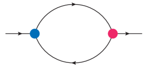
Figure 1: One-loop correction to the scalar propagator arising from the interactions of chiral multiplets.

At one-loop level there exists a single purely scalar superfield propagator correction, shown in fig. 1; it contains one chiral and one anti-chiral vertex, each of which is proportional to the modified structure constant $f_{\beta}$ found in eq. (20). Evaluating the sum over the color indices it is not difficult to find that

$${\rm fig.}~{}\ref{1loopprop}\propto|h|^{2}\left(1-\frac{1}{N^{2}}|q-q^{-1}|^{2}\right)\ .$$ (36)

Finiteness of the 1-loop correction to the chiral superfield propagator requires that, after the contribution of the internal vector multiplet is added, the UV divergence of the scalar two-point function is proportional to

$$\langle\Phi^{i}(p){\bar{\Phi}}_{j}(-p)\rangle\big{|}_{\rm 1-loop}\propto\frac{1}{\epsilon}\,\delta^{i}_{j}\,p^{2}\,\left[g_{{}_{YM}}^{2}-|h|^{2}\left(1-\frac{1}{N^{2}}|q-q^{-1}|^{2}\right)\right]\ ;$$ (37)

requiring that the divergence vanishes implies immediately that eq. (11) must be satisfied.

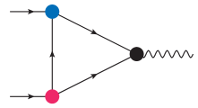
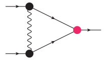
Figure 2: One-loop correction to three-point vertices.

This argument may be extended to the two-loop correction to the propagator of the chiral superfields. To this end we notice that $U(1)$ charge conservation forbids any contributions containing only scalar interactions. We are therefore to identity the diagrams containing the smallest number of internal vector multiplet lines; it is straightforward to see that one such line is sufficient. The second important observation is that any such two-loop propagator correction necessarily contains a triangle subintegral. The two possible subintegrals are shown in fig. 2; their corresponding color structures are

$${\rm fig.}~{}\ref{vert1}\propto\,g_{{}_{YM}}\,|h|^{2}\,\left(1-\frac{1}{N^{2}}|q-q^{-1}|^{2}\right)f^{abc}\quad,\quad{\rm fig.}~{}\ref{vert2}\propto\,g_{{}_{YM}}^{2}\,h\,f_{\beta}^{abc}\ .$$ (38)

This implies that, from a color space perspective, two-loop propagator corrections reduce to a one-loop analysis. Moreover, the vertex correction in fig. 2 generates an additional $q$-dependent factor when inserted into a propagator correction. We therefore conclude that the divergent part of the two-loop correction to the scalar superfield propagator due to diagrams with the smallest number of vector multiplets is proportional to

$$\frac{1}{\epsilon}\,\delta^{i}_{j}\,p^{2}\,g_{{}_{YM}}^{2}|h|^{2}\left(1-\frac{1}{N^{2}}|q-q^{-1}|^{2}\right)\ .$$ (39)

Requiring that this divergence is cancelled at $q=1$ by diagrams with further vector multiplet lines implies that

$$\langle\Phi^{i}(p){\bar{\Phi}}_{j}(-p)\rangle\big{|}_{\rm 2-loop}\propto\frac{1}{\epsilon}\delta^{i}_{j}\,p^{2}\,g_{{}_{YM}}^{2}\,\left[g_{{}_{YM}}^{2}-|h|^{2}\left(1-\frac{1}{N^{2}}|q-q^{-1}|^{2}\right)\right]\ .$$ (40)

Thus, the condition of one-loop finiteness also implies finiteness at two loops.

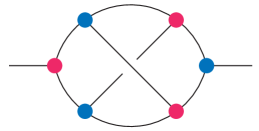
Figure 3: Three-loop correction to the scalar propagator arising from the interactions of chiral multiplets and containing only box sub-integrals. This color space contribution is not reducible to lower-loop structures.

The same type of arguments imply that, at three loop order, there exists a color structure which is different from those that appear at one and two loops. This is a consequence of the fact that at this loop order there exists a Feynman diagram, shown in fig. 3, which does not contain any triangle subintegrals and hence cannot be reduced to lower-loop structures. It is not difficult to find that

$${\rm fig.}~{}\ref{3loopprop}\propto|h|^{6}\left(N-\frac{4}{N}\right)|q-q^{-1}|^{4}\left(\left(q^{2}+4+q^{-2}\right)+\frac{5}{N^{2}}|q-q^{-1}|^{2}\right)\ .$$ (41)

Clearly, such a divergence cannot be cancelled unless the coefficient $h$ receives further corrections compared to its one- and two-loop expression (11). Apart from the three-loop propagator corrections, to determine the change to the conformal invariance condition (11) the precise form of the two-loop divergence is also necessary.

3.3 Supersymmetric relations

Supersymmetry imposes strong constraints on the structure of amplitudes in the $\beta$-deformed theory; these constraints are, to some extent, common to all ${\cal N}=1$ supersymmetric theories. Since we will be mostly interested in four-point amplitudes, let us review the consequences of supersymmetry Ward identities have on them.

In the ${\cal N}=4$ theory all four-point amplitudes fit inside a single superamplitude, i.e. they are all related to each other by ${\cal N}=4$ supersymmetry transformations. Color-ordered four-point superamplitude is given by [49, 50]

$${\bf A}_{4}^{{\cal N}=4}={\bf A}_{4}^{{\cal N}=4,(0)}M_{4}(s,t)\ ,$$ (42)

where ${\bf A}_{4}^{{\cal N}=4,(0)}$ is the tree-level color-ordered superamplitude.

In the presence of the deformation the various helicity states can be organized in four ${\cal N}=1$ superfields and their conjugates:

$$V=g^{+}+\eta\psi^{4}\qquad\quad\Phi^{ij}=\phi^{ij}+\eta\,\psi^{ij4}~{}~{}~{}~{}~{}i,j=1,2,3$$ (43)

$$V^{\dagger}=g^{-}+{\bar{\eta}}\,\psi^{ijk}\qquad\Phi^{\dagger}_{ij}={\bar{\phi}}_{ij}+{\bar{\eta}}\psi_{ij4}=\epsilon_{ijk}(\phi^{k4}+{\bar{\eta}}\psi^{k})\ .~{}~{}~{}~{}i\neq j\neq k$$ (44)

The superfield $V$ containing the gauge fields and the gauginos is denoted by $\Phi$ in [48]; we have labeled the superfields containing the scalar fields and their partners with the same labels as those of the scalar fields in the ${\cal N}=4$ theory. To preserve the similarity with the ${\cal N}=4$ theory one may additionally Fourier-transform ${\bar{\eta}}$.

The ${\cal N}=1$ supersymmetry Ward identities [51] are much less restrictive than their ${\cal N}=4$ counterparts. For example, since no sequence of transformations maps a positive helicity gluon into a negative helicity one, color-ordered amplitudes related by interchanging helicities of gluons – e.g. $A(1g^{+}2g^{+}3g^{-}4g^{-})$ and $A(1g^{+}2g^{-}3g^{+}4g^{-})$ – are not necessarily related beyond tree level. Consequently, up to CPT conjugation, the independent four-point amplitudes are

$$VVV^{\dagger}V^{\dagger}~{},~{}VV^{\dagger}\Phi\Phi^{\dagger}~{},~{}V\Phi\Phi^{\prime}\Phi^{\prime\prime}~{},~{}V\Phi^{\dagger}\Phi^{\prime\dagger}\Phi^{\prime\prime\dagger}~{},~{}\Phi\Phi^{\dagger}\Phi\Phi^{\dagger}~{},~{}\Phi\Phi^{\dagger}\Phi^{\prime\dagger}\Phi^{\prime}~{},$$ (45)

together with all their noncyclic permutations. Here $\Phi$, $\Phi^{\prime}$ and $\Phi^{\prime\prime}$ stand for different chiral multiplets (44). Conservation of the three $U(1)$ charges introduces the same selection rules as the $SU(4)$ R-symmetry of the undeformed theory; in particular, it requires that amplitudes with three vector multiplets and one chiral multiplet vanish identically. For this reason field configurations with nonvanishing charges are not listed in eq. (45).

At the expense of introducing spurious poles in external momentum invariants, one may always extract some ratio of spinor products which accounts for the phase weight determined by the helicities of the external fields. Through two-loop level, it appears however that the following relations are naturally satisfied:

$$VVVV: \mathcal{A}^{\text{extra}}_{4}(V_{1}V_{2}^{\dagger}V_{3}V_{4}^{\dagger})\propto\mathcal{A}^{{\cal N}=4,(0)}_{4}(V_{1}V_{2}^{\dagger}V_{3}V_{4}^{\dagger})$$

$$VV\Phi\,{\Phi}^{\dagger}: \mathcal{A}^{\text{extra}}_{4}(V_{1}V_{2}^{\dagger}\Phi_{3}\Phi_{4}^{\dagger})\propto\frac{\langle 23\rangle^{2}}{\langle 13\rangle^{2}}$$

$$V\Phi\,\Phi\,\Phi: \mathcal{A}^{\text{extra}}_{4}(V_{1}\Phi_{2}\Phi_{3}\Phi_{4})\propto\mathcal{A}^{\beta,(0)}_{4}(V_{1}\Phi_{2}\Phi_{3}\Phi_{4})$$

$$\Phi\,\Phi^{\dagger}\Phi\,\Phi^{\dagger}: \mathcal{A}^{\text{extra}}_{4}(\Phi_{1}\Phi^{\dagger}_{2}\Phi_{3}\Phi^{\dagger}_{4})\propto 1$$

$$\Phi\Phi^{\dagger}\Phi^{\prime}\Phi^{\prime\dagger}: \mathcal{A}^{\text{extra}}_{4}(\Phi_{1}\Phi^{\dagger}_{2}\Phi^{\prime}_{3}\Phi^{\prime\dagger}_{4})\propto 1$$

with other field configurations being obtained by simple relabeling following the noncyclic permutations of external fields.

3.4 Non-planar inheritance

While at higher orders in the $1/N$ expansion amplitudes in the deformed theory differ substantially from those of the undeformed one, the leading term in the multi-color expansion of certain multi-trace amplitudes with special configurations of external R-charges is nevertheless inherited from the undeformed theory.

Let us consider an $L$-loop single-trace planar scattering amplitude with $(2m+n)$ external lines and let us assume that the R-charges of the $(2m)$ external lines are such that this amplitude contributes to an $m$-particle cut of an $m$-loop amplitude. We will focus on the leading double-trace terms captured by such a generalized cut, which is illustrated in fig. 4 for $n=4$. We will see that, for a suitable choice of R-charges for the external lines, all $\beta$-dependence drops out of this cut, implying that the particular double-trace structure captured by it is unaffected by the deformation.

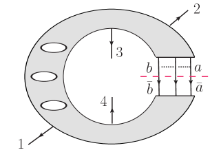
Figure 4: Generalized cut showing that, if $q_{1}+q_{2}=-q_{3}-q_{4}=0$, the leading $1/N$ term in the ${\rm Tr}_{12}{\rm Tr}_{34}$ double-trace amplitude in the $\beta$-deformed theory is proportional to the corresponding ${\cal N}=4$ amplitude.

Let us therefore analyze the phase of the relevant tree-level graph and cast it into a form suitable for the evaluation of this cut, which singles out ${\rm Tr}[T^{a_{1}}\dots T^{a_{p}}]{\rm Tr}[T^{a_{p+1}}\dots T^{a_{n}}]$. Denoting the cut legs by $a_{i}$ and ${\bar{a}}_{i}$ with $i=1,\dots,m$ on the two sides of the cut (suggesting the fact, to be used shortly, that the R-charges of sewn legs are equal in magnitude and opposite in sign), the phase is

$$\varphi(1,\dots,p,a_{1},\dots,a_{m},p+1,\dots,n,{\bar{a}}_{m},\dots,{\bar{a}}_{1})$$ (46)

$$= \sum_{i=1}^{p}\left(q_{i}\wedge\sum_{j=i+1}^{p}q_{j}+q_{i}\wedge\sum_{j=1}^{m}q_{a_{j}}+q_{i}\wedge\sum_{j=p+1}^{n}q_{j}+q_{i}\wedge\sum_{j=m}^{1}q_{{\bar{a}}_{j}}\right)$$

$$+ \sum_{i=1}^{m}\left(q_{a_{i}}\wedge\sum_{j=i+1}^{m}q_{a_{j}}+q_{a_{i}}\wedge\sum_{j=p+1}^{n}q_{j}+q_{a_{i}}\wedge\sum_{j=m}^{1}q_{{\bar{a}}_{j}}\right)$$ (47)

$$+ \sum_{i=p+1}^{n}\left(q_{i}\wedge\sum_{j=i}^{n}q_{j}+q_{i}\wedge\sum_{j=m}^{1}q_{{\bar{a}}_{j}}\right)$$ (48)

$$+ \sum_{i=m}^{1}\left(\sum_{j=i-1}^{1}q_{{\bar{a}}_{i}}\wedge q_{{\bar{a}}_{j}}\right)\ .$$ (49)

Charge conservation removes all dependence of the charge of the cut legs from the first line above; for the same reason, the terms on the second line may also be written as

$$\sum_{i=1}^{m}\left(-q_{a_{i}}\wedge\sum_{j=1}^{p}q_{j}-q_{a_{i}}\wedge\sum_{j=1}^{i-1}q_{a_{j}}\right)\ ;$$ (50)

On the third line, the dependence on the charges of cut legs enters multiplied by $\sum_{i=p+1}^{n}q_{i}$. Finally, the sum on the fourth line may be reorganized as

$$\sum_{i=m}^{1}\sum_{j=i-1}^{1}q_{{\bar{a}}_{i}}\wedge q_{{\bar{a}}_{j}}=\sum_{j=1}^{m}\sum_{i=m}^{j+1}q_{{\bar{a}}_{i}}\wedge q_{{\bar{a}}_{j}}$$ (51)

$$= +\sum_{j=1}^{m}\sum_{i=1}^{p}q_{i}\wedge q_{{a}_{j}}+\sum_{j=1}^{m}\sum_{i=1}^{m}q_{a_{i}}\wedge q_{{a}_{j}}+\sum_{j=1}^{m}\sum_{i=p+1}^{n}q_{i}\wedge q_{{a}_{j}}-\sum_{j=1}^{m}\sum_{i=1}^{j-1}q_{{a}_{i}}\wedge q_{{a}_{j}}\ ,$$ (52)

where we also used the relation $q_{\bar{a}}=-q_{a}$. The first term on the second line combines with the first term on the right-hand side of (50). The second term on the second line vanishes, since the two charge vectors are equal. The third term on the second line cancels the second term on the third line of (49); last, the fourth term on the second line in (52) cancels the second term in (50). Combining everything, it is not difficult to see that

$$\varphi(1,\dots,p,a_{1},\dots,a_{m},p+1,\dots,n,{\bar{a}}_{m},\dots,{\bar{a}}_{1})=\sum_{i=p+1}^{n}\sum_{j=i}^{n}q_{i}\wedge q_{j}+\sum_{i=p+1}^{n}q_{i}\wedge\sum_{j=1}^{m}q_{a_{j}}\ .$$ (53)

Thus, if $\sum_{i=p+1}^{m}q_{i}=-\sum_{i=1}^{p}q_{i}=0$, the $\beta$-dependent phase of the generalized cut contributing to the double-trace structure ${\rm Tr}[T^{a_{1}}\dots T^{a_{p}}]{\rm Tr}[T^{a_{p+1}}\dots T^{a_{n}}]$ does not depend on the charges of the cut lines; consequently, this cut is the same as in the undeformed theory.

We may give a pictorial interpretation to this result. In color space, all Feynman diagrams contributing to the cut analyzed above have the topology of a cylinder, with legs $1,\dots,p$ attached to one boundary and legs $p+1,\dots,n$ attached to the other. If the total charge flowing in through one boundary, $\sum_{i=p+1}^{m}q_{i}=-\sum_{i=1}^{p}q_{i}$, vanishes, then the corresponding double-trace amplitude is not deformed apart from a potential overall phase. Examples include ${\rm Tr}_{12}{\rm Tr}_{34}$ in $\mathcal{A}_{4}^{\beta}(1g^{+},2g^{-},3\phi^{ij},4\phi^{k4})$ (with $i\neq j\neq k=1,2,3$), ${\rm Tr}_{12}{\rm Tr}_{34}$ and ${\rm Tr}_{14}{\rm Tr}_{23}$ in $\mathcal{A}_{4}^{\beta}(1\phi^{23},2\phi^{14},3\phi^{23},4\phi^{14})$ and ${\rm Tr}_{12}{\rm Tr}_{34}$ in $\mathcal{A}_{4}^{\beta}(1\phi^{23},2\phi^{14},3\phi^{13},4\phi^{24})$. This is a direct counterpart of a similar result proven in [52] for space-time non-commutative field theories. The explicit calculations in the following sections support the conclusions reached here.

It is not difficult to generalize this criterion to all multi-trace amplitudes; their color-space graphs have the topology of a sphere with as many punctures as trace factors. If the R-charge flow through all punctures vanishes, then the corresponding amplitude is the same as in the ${\cal N}=4$ theory even when $\beta\neq 0$. For example, all ${\cal O}(1/N)$ multi-trace gluon amplitudes are the same as in the undeformed theory; beginning at three-loop order, they are more convergent in the UV than the single-trace leading color terms [3].

4 $\beta$-deformed ${\cal N}=4$ sYM theory at one-loop

One loop amplitudes may be evaluated though a color-dressed generalization of the strategy applicable to all supersymmetric field theories [53], by evaluating first the coefficients of box integrals through quadruple cuts, then those of triangle integrals through triple cuts and last the coefficient of bubble integrals, which should vanish in our case up to use of eq. (11). Alternatively, they may be constructed only from their color-dressed two-particle cuts. As mentioned in (35), we will separate the ${\cal N}=4$ part of the amplitude as

$${\cal A}_{4}^{\beta,(1)}={\cal A}_{4}^{{\cal N}=4,(1)}+{\cal A}_{4}^{\text{extra},(1)}\ ,$$ (54)

where ${\cal A}_{4}^{{\cal N}=4,(1)}$ is well-known [54]:

$${\cal A}_{4}^{{\cal N}=4,(1)} = -g_{{}_{YM}}^{2}\,s_{12}s_{23}{\cal A}_{4}^{{\cal N}=4,(0)}\Big{[}N\Big{(}\mathcal{I}_{1,2,3,4}({\rm Tr}_{1234}+{\rm Tr}_{4321})+\mathcal{I}_{1,3,4,2}({\rm Tr}_{1342}+{\rm Tr}_{2431})$$ (56)

$$\qquad\qquad\qquad\qquad\qquad+\mathcal{I}_{1,4,2,3}({\rm Tr}_{1423}+{\rm Tr}_{3241})\Big{)}$$

$$\qquad+2\,\left(\mathcal{I}_{1,2,3,4}+\mathcal{I}_{1,4,2,3}+\mathcal{I}_{1,3,4,2}\right)\left({\rm Tr}_{12}{\rm Tr}_{34}+{\rm Tr}_{13}{\rm Tr}_{24}+{\rm Tr}_{14}{\rm Tr}_{23}\right)\Big{]}$$

with ${\cal I}_{1,2,3,4}$ the scalar box integral shown in fig. 5(a)

$${\cal I}_{1,2,3,4}=-i\int\frac{d^{d}l}{(2\pi)^{d}}\frac{1}{l^{2}(l-k_{1})^{2}(l-k_{1}-k_{2})^{2}(l+k_{4})^{2}}\ .$$ (57)

The terms included in ${\cal A}_{4}^{\text{extra},(1)}$ have a more complicated structure which we now discuss.

(a) ${\cal I}_{1,2,3,4}$

(b) ${\cal I}_{1,2|34}$

Figure 5: Integrals contributing to the one-loop amplitudes.

4.1 $\beta$-dependent one-loop corrections to four-point amplitudes in trace basis

As explained in § 3.3, amplitudes may be organized following the number of external lines in the vector multiplet (45). Moreover, due to minimal supersymmetry, color-stripped amplitudes related by non-cyclic permutations of external legs are independent. For each configuration of external ${\cal N}=1$ multiplets we will choose one representative and list here the corresponding complete one-loop amplitudes; each color-stripped sub-amplitude will be expressed as a sum of box and triangle integrals with the appropriate momentum-dependent coefficients.

$\bullet$ Four-gluon amplitude: As follows from the discussion in previous sections, this amplitude is not modified in the presence of the deformation:

$$\mathcal{A}_{4}^{\text{extra},(1)}(1g^{+},2g^{-},3g^{+},4g^{-})=0\ .$$ (58)

Moreover, R-charge conservation requires that the four-point three-gluon amplitude vanishes identically.

$\bullet$ Two-gluon two-scalar amplitude: As discussed in § 3.4, the first deformation-dependent correction to this amplitude has a double-trace structure and involves a nontrivial $U(1)$-charge flow between the fields in the two traces. At higher orders in the $1/N$ expansion other trace structures are deformed as well. Since such terms do not have a tree-level counterpart, the expected structure of IR divergences [23]-[37] requires that they be finite. This is indeed the case; the deformation-dependent terms are

$$\mathcal{A}^{\text{extra},(1)}_{4}(1g^{+},2g^{-},3\phi^{14},4\phi^{23})=h(g_{{}_{YM}},N,q)^{2}(q-q^{-1})^{2}\;\frac{\langle 23\rangle^{2}}{\langle 13\rangle^{2}}\;{\rm B}(1234)$$ (59)

$$\qquad\times\left[\left(1-\frac{2}{N^{2}}\right)({\rm Tr}_{13}{\rm Tr}_{24}+{\rm Tr}_{14}{\rm Tr}_{23})-\frac{1}{N}({\rm Tr}_{1324}+{\rm Tr}_{1432})-\frac{2}{N^{2}}{\rm Tr}_{12}{\rm Tr}_{34}\right]\ .$$

Here the overall factor $h(g_{{}_{YM}},N,q)^{2}$ is given by the solution to the equation (11). The terms of higher order in $1/N$ originate from the tree-level double-trace amplitudes. The momentum-dependent function ${\rm B}(1234)$ is a particular combination of box and triangle integrals (see fig. 5 for notation)

$${\rm B}(1234)=s_{12}s_{14}\mathcal{I}_{1,2,3,4}-s_{12}(\mathcal{I}_{12|3,4}+\mathcal{I}_{34|1,2})-s_{14}(\mathcal{I}_{14|2,3}+\mathcal{I}_{23|1,4})\ .$$ (60)

This expression may be written as a box integral with a Gram determinant numerator; one may also recognize it as the six-dimensional scalar box integral. Evaluating $B(1234)$ (either using the known expressions for the contributing integrals or by recognizing it as a six-dimensional integral [55]) leads to

$${\rm B}(1234)=-\frac{1}{(4\pi)^{2}}\left[\left(\ln\frac{s_{12}}{s_{23}}\right)^{2}+\pi^{2}\right]\ ,$$ (61)

which is indeed finite in the IR, as expected.

$\bullet$ One-gluon one-scalar two-fermion amplitude: The single-trace terms in this amplitude acquire, as at tree-level, $\beta$-dependent factors which depend on the specific color structure. Moreover, since any pair of fields carries nontrivial R-charge, all double-trace terms will receive $\beta$-dependent corrections. Because of this it is convenient to quote the complete amplitude rather than just ${\cal A}_{4}^{\text{extra},(1)}$:

$$\mathcal{A}_{4}^{\beta,(1)}(1g^{+},2\phi^{i4},3\psi^{j},4\psi^{k})=g_{{}_{YM}}h(g_{{}_{YM}},N,q)\;s_{12}s_{23}\;\mathcal{A}_{4}^{\beta,(0)}(1g^{+},2\phi^{i4},3f^{j},4f^{k})\Big{[}$$ (62)

$$\qquad\qquad\times N\left(\mathcal{I}_{1,2,3,4}\left[q\,{\rm Tr}_{1234}+q^{-1}\,{\rm Tr}_{1432}\right]+\mathcal{I}_{1,2,4,3}\left[q^{-1}\,{\rm Tr}_{1243}+q\,{\rm Tr}_{1342}\right]\right.$$ (63)

$$\left.\qquad\qquad\qquad\qquad\qquad\qquad\qquad\qquad\qquad\qquad\qquad+\mathcal{I}_{1,3,2,4}\left[q^{-1}\,{\rm Tr}_{1324}+q\,{\rm Tr}_{1423}\right]\right)$$ (64)

$$\qquad\qquad\quad+(q+q^{-1})\left(\mathcal{I}_{1,2,3,4}+\mathcal{I}_{1,2,4,3}+\mathcal{I}_{1,3,2,4}\right)\left[{\rm Tr}_{14}{\rm Tr}_{23}+{\rm Tr}_{13}{\rm Tr}_{24}+{\rm Tr}_{12}{\rm Tr}_{34}\right]\Big{]}\ .$$

The double-trace $1/\epsilon^{2}$ poles vanish identically, as in the underformed theory, as required by the absence of a tree-level double-trace amplitude with only one field in the vector multiplet (23). The remaining double-trace $1/\epsilon$ terms introduce $\beta$-dependence in the soft anomalous dimension matrix.

There are two independent four-point amplitudes with four fields in the chiral multiplet: those in which all fields belong to one multiplet and its conjugate and amplitudes in which the fields belong to two different chiral multiplets. We will choose $\mathcal{A}(1\phi^{23},2\phi^{14},3\phi^{23},4\phi^{14})$ and $\mathcal{A}(1\phi^{23},2\phi^{14},3\phi^{13},4\phi^{24})$ as representatives of these two cases, respectively.

$\bullet$ like-charge four-scalar amplitude: At ${\cal O}(1/N)$ these amplitudes are rather constrained; for the amplitude $\mathcal{A}(1\phi^{23},2\phi^{14},3\phi^{23},4\phi^{14})$ the discussion in § 3.4 allows a nonzero value only for the ${\rm Tr}_{13}{\rm Tr}_{24}$ structure. At higher orders in $1/N$ however all trace structures may be corrected. We find that

$$\mathcal{A}^{\text{extra},(1)}(1234) = g_{{}_{YM}}^{2}\Big{[}\;N\Big{(}-1+{\tilde{h}}^{4}+\frac{4{\tilde{h}}^{4}}{N^{2}}(q-q^{-1})^{2}\Big{)}\,[{\rm Tr}_{1234}+{\rm Tr}_{1432}]$$

$$\qquad\;\,\,-\frac{1}{N}{\tilde{h}}^{4}(q-q^{-1})^{2}(q^{2}+q^{-2})\,[{\rm Tr}_{1324}+{\rm Tr}_{1423}+{\rm Tr}_{1243}+{\rm Tr}_{1342}]$$

$$\quad+\Big{(}-2+2{\tilde{h}}^{4}+\frac{1}{N^{2}}{\tilde{h}}^{4}(q-q^{-1})^{4}\Big{)}\,[{\rm Tr}_{14}{\rm Tr}_{23}+{\rm Tr}_{12}{\rm Tr}_{34}]$$

$$\qquad\qquad\;+\big{(}-2+{\tilde{h}}^{4}(q^{4}+q^{-4})\big{)}\;{\rm Tr}_{13}{\rm Tr}_{24}\Big{]}\;{\rm B}(1234)\ ,$$

where ${\tilde{h}}=g_{{}_{YM}}^{-1}h(g_{{}_{YM}},N,q)$ and ${\rm B}(1234)$ is defined in (60). Using (11) it is easy to see that the first and third line are ${\cal O}(1/N)$ and ${\cal O}(1/N^{2})$ respectively, as required by the discussion in § 3.4. Since these terms are proportional to the combination of integrals in eq. (60) these corrections are IR-finite, as required by the analysis in § 2.3.

$\bullet$ different-charge four-scalar amplitude: While only two two-trace structures are corrected at ${\cal O}(1/N)$, all trace structures are corrected at higher orders. For the field configuration $\mathcal{A}(1\phi^{23},2\phi^{14},3\phi^{13},4\phi^{24})$, the various color-ordered terms are as follows:

$${A}_{4;2}^{\text{extra},(1)}(14;23) = g_{{}_{YM}}^{2}\Big{(}-1+\frac{1}{2}{\tilde{h}}^{4}(q^{4}+q^{-4})+\frac{1}{2N^{2}}{\tilde{h}}^{4}(q-q^{-1})^{4}\Big{)}\;{\rm B}(1234)$$ (67)

$$+g_{{}_{YM}}^{2}\big{(}-2+{\tilde{h}}^{2}(q^{2}+q^{-2})\big{)}(s_{12}s_{13}\mathcal{I}_{1,2,4,3}-s_{14}s_{13}\mathcal{I}_{1,3,2,4})$$

$${A}_{4;2}^{\text{extra},(1)}(13;24) = g_{{}_{YM}}^{2}(-1+{\tilde{h}}^{4}){\rm B}(1234)$$ (68)

$$+ g_{{}_{YM}}^{2}\big{(}-2+{\tilde{h}}^{2}(q^{2}+q^{-2})\big{)}\mathcal{I}_{1,2,4,3}+2g_{{}_{YM}}^{2}(1-{\tilde{h}}^{2})\mathcal{I}_{1,3,2,4}$$ (69)

$${A}_{4;2}^{\text{extra},(1)}(12;34) = g_{{}_{YM}}^{2}\Big{(}-1+{\tilde{h}}^{4}+\frac{1}{2N^{2}}{\tilde{h}}^{4}(q-q^{-1})^{4}\Big{)}\;{\rm B}(1234)$$ (71)

$$\quad+2g_{{}_{YM}}^{2}(-1+{\tilde{h}}^{2})(s_{12}s_{13}\mathcal{I}_{1,2,4,3}-s_{14}s_{13}\mathcal{I}_{1,3,2,4})$$

$${A}_{4;1}^{\text{extra},(1)}(1234) = {A}_{4;1}^{\text{extra},(1)}(1432)=\frac{g_{{}_{YM}}^{2}}{2}N\Big{(}-1+{\tilde{h}}^{4}-\frac{1}{N^{2}}{\tilde{h}}^{4}(q-q^{-1})^{4}\Big{)}\;{\rm B}(1234)$$ (72)

$${A}_{4;1}^{\text{extra},(1)}(1243) = {A}_{4;1}^{\text{extra},(1)}(1342)$$ (73)

$$= \frac{g_{{}_{YM}}^{2}}{N}{\tilde{h}}^{4}(q-q^{-1})^{2}\;{\rm B}(1234)+\frac{g_{{}_{YM}}^{2}}{N}{\tilde{h}}^{2}(q-q^{-1})^{2}s_{13}s_{14}\mathcal{I}_{1,3,2,4}$$ (74)

$${A}_{4;1}^{\text{extra},(1)}(1324) = {A}_{4;1}^{\text{extra},(1)}(1423)^{*}=-\frac{g_{{}_{YM}}^{2}}{N}{\tilde{h}}^{4}(q-q^{-1})^{2}q^{2}\;{\rm B}(1234)$$

$$\!\!\!\!\!\!\!\!\!\!\!\!\!\!\!\!\!\!\!\!\!\!\!\!\!\!\!\!\!\!\!\!\!\!\!\!\!\!\!\!\!-\frac{g_{{}_{YM}}^{2}}{N}{\tilde{h}}^{2}(q-q^{-1})^{2}s_{12}s_{13}\mathcal{I}_{1,2,4,3}+\frac{g_{{}_{YM}}^{2}}{N}\Big{(}N^{2}(1-{\tilde{h}}^{2}q^{2})+{\tilde{h}}^{2}(q-q^{-1})^{2}\Big{)}s_{13}s_{14}\mathcal{I}_{1,3,2,4}$$

where, as before, ${\tilde{h}}=g_{{}_{YM}}^{-1}h(g_{{}_{YM}},N,q)$. The ${\cal O}(N)$ term in eq. (4.1) combines with the undeformed amplitude to produce the $\beta$-dependent phase factor appropriate for a single-trace planar amplitude. The charge assignment forbids similar phase factors for the other single-trace amplitudes. All triangle integrals may be combined in the six-dimensional box integral ${\rm B}(1234)$. It is not difficult to see that a leading IR divergence exists, as expected, only for trace structures that have a tree-level counterpart, cf. § 2.3.

4.2 One-loop amplitudes in the modified structure constant basis

The results described above may also be organized in terms of the modified structure constants (20). The resulting expressions may also be obtained directly in this basis by using tree-level amplitudes dressed with the structure constants $f_{\beta}$ in unitarity cuts. Similarly to the undeformed case, some of the complexity of the expressions in § 4.1 is absorbed in the contraction of structure constants.

An inspection of the unitarity cuts and of the tree-level amplitudes in this representation reveals that five combinations of modified structure constants can appear:

$$\kappa_{\beta}(1234;q) = {h}(g_{{}_{YM}},N,q)f^{a_{1}bc}f^{a_{2}cd}f^{a_{3}de}f_{\beta}^{a_{4}ea}$$ (76)

$$\kappa_{0}(1234;q) = {h}(g_{{}_{YM}},N,q)^{2}f^{a_{1}bc}f^{a_{2}cd}f_{\beta}^{a_{3}de}f_{-\beta}^{a_{4}ea}$$ (77)

$$\kappa_{1}(1234;q) = {h}(g_{{}_{YM}},N,q)^{4}f_{\beta}^{a_{1}bc}f_{-\beta}^{a_{2}cd}f_{-\beta}^{a_{3}de}f_{\beta}^{a_{4}ea}$$ (78)

$$\kappa_{2}(1243;q) = \kappa_{0}(1243;q^{-1})={h}(g_{{}_{YM}},N,q)^{2}f^{a_{1}bc}f^{a_{2}cd}f_{-\beta}^{a_{4}de}f_{\beta}^{a_{3}ea}$$ (79)

$$\kappa_{3}(1324;q) = {h}(g_{{}_{YM}},N,q)^{2}f^{a_{1}bc}f^{a_{3}cd}f_{\beta}^{a_{2}de}f_{\beta}^{a_{4}ea}~{},$$ (80)

where ${h}(g_{{}_{YM}},N,q)$ is the coefficient of the superpotential which renders the theory UV-finite, given by the solution to eq. (11) at one- and two-loop order. Other products of structure constants not involving the deformation parameter also appear. Below we will focus on the $\beta$-dependent terms which will depend on differences between various $\kappa$ factors for generic $q$ and for $q=1$. While in general the translation of products of structure constants to the trace basis does not involve terms proportional to $N^{-2}$, such terms nevertheless appear due to the structure of ${h}(g_{{}_{YM}},N,q)$. For example, one may check that

$$\kappa_{0}(1234;q)={h}(g_{{}_{YM}},N,q)^{2}\Big{[}\;2{\rm Tr}_{12}{\rm Tr}_{34}+N({\rm Tr}_{1234}+{\rm Tr}_{1432})$$

$$+ (q+q^{-1})({\rm Tr}_{13}{\rm Tr}_{24}+{\rm Tr}_{14}{\rm Tr}_{23})+\frac{1}{N}(q-q^{-1})^{2}({\rm Tr}_{1234}-{\rm Tr}_{1324}-{\rm Tr}_{1423}+{\rm Tr}_{1432})\Big{]}\ ,$$

implying that

$$\mathcal{A}^{\text{extra},(1)}_{4}(1g^{+},2g^{-},3\phi^{23},4\phi^{14})=\left(\kappa_{0}(1234;q)-\kappa_{0}(1234;1)\right){\rm B}(1234)\ .$$ (82)

The $q$ dependence of ${h}(g_{{}_{YM}},N,q)$ participates nontrivially in this relation.

One may similarly show that the other one-loop amplitudes evaluated in the previous section can be written as

$$\mathcal{A}_{4}^{\beta,(1)}(1g^{+},2\phi^{i4},3\psi^{j},4\psi^{k}) = g_{{}_{YM}}s_{12}s_{23}A^{(0)}_{4}(1234)\Big{(}\kappa_{\beta}(1234;q)\,{\cal I}^{4}_{1,2,3,4}$$ (84)

$$+\kappa_{\beta}(1423;q)\,{\cal I}^{4}_{1,4,2,3}+\kappa_{\beta}(1342;q)\,{\cal I}^{4}_{1,3,4,2}\Big{)}\ ,$$

$$\mathcal{A}^{\text{extra},(1)}(1\phi^{23},2\phi^{14},3\phi^{23},4\phi^{14}) = \frac{1}{2}\left(\kappa_{0}(1234;q)-\kappa_{0}(1234;1)\right){\rm B}(1234)\ ,$$ (85)

$$\mathcal{A}^{\text{extra},(1)}(1\phi^{23},2\phi^{14},3\phi^{13},4\phi^{24}) = g_{{}_{YM}}^{-2}\left(\kappa_{1}(1234;q)-\kappa_{1}(1234;1)\right)\,{\rm B}(1234)$$ (86)

$$+ \left(\kappa_{2}(1243;q)-\kappa_{2}(1243;1)\right)\,s_{12}s_{24}\,{\cal I}^{4}_{1,2,4,3}$$ (87)

$$+ \left(\kappa_{3}(1324;q)-\kappa_{3}(1324;1)\right)\,s_{13}s_{23}\,{\cal I}^{4}_{1,3,2,4}\ .$$ (88)

The $q$ factors dressing each color structure depend on the charges of virtual particles; it turns out that, in the amplitudes in eqs. (82) and (85), the internal charge configuration is symmetric. One may use the identity

$$\kappa_{0}(1234;q)-\kappa_{0}(1234;1)\mapsto\frac{1}{2}\left(\kappa_{0}(1234;q)+\kappa_{0}(1234;q^{-1})-2\kappa_{0}(1234;1)\right)$$ (89)

to make this symmetry manifest. Similar identities do not seem to exist for the other combinations of structure constants, which is consistent with the internal charge configurations for the different-charge scalar amplitudes not being symmetric.

With the one-loop amplitudes written in this color basis it is not difficult to search for the color/kinematic duality. The amplitude in eq. (84), whose color factors obey the Jacobi identity, may be easily seen to indeed exhibit it: similarly to the undeformed theory, Jacobi transformations map the three terms into each other. Other amplitudes however, such as (82), are not invariant under Jacobi transformations. One may trace this both to the absence of Jacobi identities for color factors as well as to the presence of both box and triangle integrals with the same color factor.

4.3 The symmetries of the one-loop four-point amplitudes

Similarly to ${\cal N}=4$ one-loop amplitudes, the one-loop amplitudes of the $\beta$-deformed theory have certain symmetries, in some cases only after certain state-dependent rational functions of spinor products are extracted. Some of these symmetries are dictated by the configuration of external legs. For example, one may expect that ${\cal A}^{\beta}_{4}(1\phi^{jk},2\phi^{i4},3\phi^{jk},4\phi^{i4})$ with $i\neq j\neq k=1,2,3$ (i.e. an amplitude with all external states carrying the same type of $U(1)$ charge) is invariant under conjugation together with a certain relabeling of momenta (the color factors are not relabeled):

$${\rm C}:~{}\langle\rangle\leftrightarrow[]\quad\{1,2,3,4\}\mapsto\{2,1,4,3\}\qquad\text{or}\qquad{\rm C}^{\prime}:~{}\langle\rangle\leftrightarrow[]\quad\{1,2,3,4\}\mapsto\{4,3,2,1\}\ .$$ (90)

It is not difficult to check that this is indeed a symmetry of eq. (4.1). This amplitude has further symmetries stemming from its external states being identical in pairs; one may check that, indeed, eq. (4.1) is invariant under the relabeling

$$1\leftrightarrow 3\qquad\text{or}\qquad 2\leftrightarrow 4\ .$$ (91)

For some of the single-trace components, these symmetries may be also identified as a consequence of the inversion symmetry of scattering amplitudes: $A(1,\dots,n)=(-1)^{n}A(n,\dots,1)$. For the double-trace terms these transformations are symmetries of the color structures, which suggests that they should also be symmetries of the kinematic part.

Similarly, the two-gluon two-scalar amplitude $\mathcal{A}(1g^{+},2g^{-},3\phi^{ij},4\phi^{kl})$ ($i\neq j\neq k\neq l$) has two independent symmetries. One of them, present also in the tree-level amplitude, is the ${\rm C}$ transformation in eq. (90). The second one is a symmetry of the amplitude only after the factor $\langle 23\rangle^{2}/\langle 13\rangle^{2}$ is stripped off; by inspecting the remainder it is not difficult to see that it is invariant under

$${\rm U}:\{1,2,3,4\}\mapsto\{4,3,2,1\}\qquad\qquad{\rm U}^{\prime}:\{1,2,3,4\}\mapsto\{3,4,1,2\}\ .$$ (92)

It is not difficult to see that ${\rm U}^{\prime}={\rm U}{\rm C}$ and ${\rm U}={\rm U}^{\prime}{\rm C}$. While these are symmetries of amplitudes with identical external states (being in fact a simple inversion (U) or a shift transformation by two units (U’)), it is not clear why it should survive in the presence of the deformation, when the external states belong to different multiplets. This feature suggests that certain four-point amplitudes exhibit more supersymmetry than the complete theory. Technically, this symmetry arises because for chargeless and like-charge external states the internal states are symmetric under the exchange of internal states with charges different from that of the external one. As we will see, the leading two-loop double-trace terms exhibit this symmetry as well. An analysis of cuts of higher loop amplitudes shows that this symmetry may survive at two loop level and beyond.

5 The leading double-trace correction to a two-loop amplitude

The UV properties of the one-loop amplitudes constructed in the previous section are in line with the expectations based on the finiteness of the theory and the consequences of ${\cal N}=1$ supersymmetry. Quite generally however, one-loop amplitudes do not always accurately reflect the properties of higher-loop amplitudes. For example, the one-loop amplitudes of the ${\cal N}=4$ sYM theory do not follow the same pattern as higher-loop amplitudes and diverge in $D_{c}=8$ dimensions and not in $D_{c}=10$ as suggested by the usual expression of the critical dimension [56, 58]

$$D_{c}^{{\cal N}=4}=4+\frac{6}{L}\ .$$ (93)

While one-loop amplitudes follow the pattern of critical dimensions suggested by ${\cal N}=1$ supersymmetry, it is nevertheless interesting to explore whether some unexpected features emerge in the $\beta$-deformed theory as well. As we will see, this is indeed the case.

5.1 Generalities

We will consider here in detail the four-point amplitudes with two fields in the vector multiplet and focus on the leading terms arising due to the presence of the deformation – the double-trace terms in this amplitude. We will organized them as

$$\mathcal{A}^{\beta,(2)}_{4}(1g^{+},2g^{-},3\phi^{i4},4\phi^{jk}) = \mathcal{A}^{{\cal N}=4,(2)}_{4}(1234)+\mathcal{A}^{\text{extra},(2)}_{4}(1234)$$ (94)

$$\mathcal{A}^{\text{extra},(2)}_{4}(1234) = (q^{2}+q^{-2}-2)\frac{\langle 23\rangle^{2}}{\langle 13\rangle^{2}}\mathcal{M}^{\text{extra},(2)}_{4}(1234)\ ,$$ (95)

where $i\neq j\neq k=1,2,3$. For the field configuration discussed here, the term proportional to ${\rm Tr}_{12}{\rm Tr}_{34}$ is absent as there is no $U(1)$-charge flow between fields in the two trace factors. As discussed in § 3.4, the corresponding correction vanishes identically. Thus, the first $\beta$-dependent correction to the scalar factor has the form:

$$\mathcal{M}^{\text{extra},(2)}_{4}(1234)={M}^{\text{extra},(2)}_{13;24}{\rm Tr}_{13}{\rm Tr}_{24}+{M}^{\text{extra},(2)}_{14;23}{\rm Tr}_{14}{\rm Tr}_{23}\ .$$ (96)

An expression in terms of products of modified structure constants (20) should also exist once higher order terms in the $1/N$ expansion are included.

Similarly to the ${\cal N}=4$ amplitudes, each trace structure may be expressed as a sum of parent integrals (i.e. in this case the planar and non-planar massless double-box integrals) each of them having a certain kinematic numerator factor:

$$M^{\text{extra},(2)}_{*;*}=\sum_{i}c_{i}I_{i}\ .$$ (97)

The numerator factors $c_{i}$ contain inverse propagators; they cancel some of the propagators appearing in the parent graphs, thus leading to contact terms. As discussed at length in [2, 3], there is no unique assignment of contact terms to parent graphs; for this reason we will write out explicitly the contact terms. Even more so than in ${\cal N}=4$ sYM theory, the proliferation of contact terms implies that there are many superficially different presentations of amplitudes in theories with reduced supersymmetry. Symmetries provide an efficient way of organizing the result. The two-loop amplitude is expected to be invariant under the ${\rm C}$ transformation in eq. (90); in fact, the spinor ratio factor and the scalar function ${\cal M}$ are separately invariant under this symmetry.

It is possible to see that the transformations (92) are symmetries of the generalized cuts of the two-loop contribution to the scalar function ${\cal M}$. Moreover, the cuts of ${M}^{\text{extra},(2)}_{14;23}$ can be saturated by cuts of integrals whose topologies are manifestly invariant under ${\rm U}$ but not invariant under ${\rm U}^{\prime}$ while the cuts of ${M}^{\text{extra},(2)}_{13;24}$ can be saturated by cuts of integrals whose topologies are manifestly invariant under ${\rm U}^{\prime}$ but not invariant under ${\rm U}$. It is therefore natural to enforce a different manifest symmetry on the kinematic numerators in the two components of the scalar function.

5.2 ${M}^{\text{extra},(2)}_{14;23}$

The integral topologies entering the $\beta$-dependent contribution to the color-stripped amplitude corresponding to the trace structure ${\rm Tr}_{14}{\rm Tr}_{23}$ are shown in figure 6. Only the first three are invariant under the complete symmetry (90), (92); some of the integrals for which ${\rm C}$ is not a symmetry are invariant under either ${\rm U}$ or ${\rm U}^{\prime}$ transformations and vice versa. We will choose to organize the result in a form that is manifestly invariant under ${\rm C}$ and ${\rm U}$:

$$M^{\text{extra},(2)}_{14;23}=\sum_{i}\alpha_{i}I_{i}+(1+{\rm C})\sum_{i}\beta_{i}J_{i}+(1+{\rm U})\sum_{i}\gamma_{i}K_{i}+(1+{\rm U})(1+{\rm C})\sum_{i}\delta_{i}L_{i}\ ,$$ (98)

with invariance under ${\rm U}^{\prime}$ following from the relation ${\rm U}^{\prime}={\rm U}{\rm C}$. Given some collection of integrals, there are other ways to make it invariant under ${\rm C}$ and ${\rm U}$; the expression here is singled out by the explicit calculation.

(a) $I_{1}$

(b) $I_{2}$

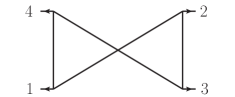
(c) $I_{3}$

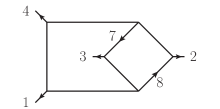
(d) $J_{1}$

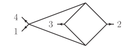
(e) $J_{2}$

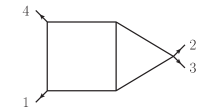
(f) $J_{3}$

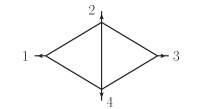
(g) $J_{4}$

(h) $J_{5}$

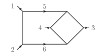
(i) $K_{1}$

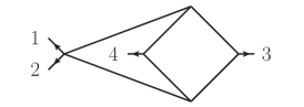
(j) $K_{2}$

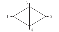
(k) $K_{3}$

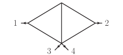
(l) $K_{4}$

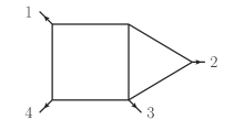
(m) $L_{1}$

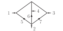
(n) $L_{2}$

Figure 6: Integrals contributing to the trace structure ${\rm Tr}_{14}{\rm Tr}_{23}$ in the two-gluon two-scalar amplitude. Their coefficients are listed in eqs.(101)-(112).

With the definition $\tau_{a,b}=2k_{a}\cdot k_{b}$ ($k_{a}$ with $a\geq 5$ are loop momenta), the numerator factors of the various integrals are:

$$\alpha_{1} = \tau_{1,4}\left(\tau_{1,8}^{2}+\tau_{2,5}^{2}+\tau_{4,7}^{2}+\tau_{3,6}^{2}+\tau_{1,2}(\tau_{1,8}+\tau_{2,5}+\tau_{4,7}+\tau_{3,6}-2\tau_{1,4})-\tau_{1,8}\tau_{2,5}-\tau_{4,7}\tau_{3,6}\right)$$ (99)

$$\alpha_{2} = \tau_{1,4}\left(\tau_{1,8}^{2}+\tau_{2,6}^{2}+\tau_{4,7}^{2}+\tau_{3,5}^{2}+\tau_{1,2}(\tau_{1,8}+\tau_{2,6}+\tau_{4,7}+\tau_{3,5})+\tau_{1,8}\tau_{2,6}+\tau_{4,7}\tau_{3,5}\right)$$ (100)

$$\alpha_{3} = -4\tau_{1,3}\tau_{1,4}$$ (101)

$$\beta_{1} = 2\tau_{1,4}\left(\tau_{1,8}^{2}+\tau_{4,7}^{2}+\tau_{1,3}(\tau_{1,8}+\tau_{4,7})\right)$$ (102)

$$\beta_{2} = -2\tau_{1,4}^{2}$$ (103)

$$\beta_{3} = 2\tau_{1,4}^{2}$$ (104)

$$\beta_{4} = 2\tau_{1,2}$$ (105)

$$\beta_{5} = \tau_{1,4}-2\tau_{1,2}$$ (106)

$$\gamma_{1} = \tau_{1,2}\left(\tau_{1,5}^{2}+\tau_{2,6}^{2}+\tau_{1,2}(\tau_{1,5}+\tau_{2,6})\right)$$ (107)

$$\gamma_{2} = 2\tau_{1,2}^{2}$$ (108)

$$\gamma_{3} = 2\tau_{1,2}$$ (109)

$$\gamma_{4} = \tau_{1,3}-\tau_{1,2}$$ (110)

$$\delta_{1} = \tau_{1,4}^{2}$$ (111)

$$\delta_{2} = -\tau_{1,4}\tau_{2,5}+\textstyle{\frac{1}{2}}\tau_{12}(3\tau_{1,3}+\tau_{2,5}-2\tau_{3,5}+2\tau_{2,7})$$ (112)

Integration-by-parts identities may be used to reduce some of the integrals with nontrivial numerator factors to simpler ones along the lines of [57]. We will however not pursue this here. It is not difficult to see that, integral by integral, ${M}^{\text{extra},(2)}_{14;23}$ is UV finite in four dimensions. All the integrals having at least one four-point vertex may be obtained (in several ways) by collapsing suitable internal lines in the graphs $I_{1},I_{2},J_{1},K_{1}$ and their images under the symmetries of the amplitude.

5.3 ${M}^{\text{extra},(2)}_{13;24}$

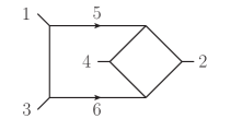
(a) $J^{\prime}_{1}$

(b) $J^{\prime}_{2}$

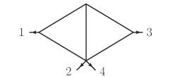
(c) $J^{\prime}_{3}$

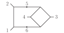
(d) $K^{\prime}_{1}$

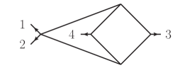
(e) $K^{\prime}_{2}$

(f) $L^{\prime}_{1}$

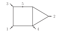
(g) $M^{\prime}_{1}$

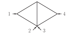
(h) $X^{\prime}_{1}$

(i) $Y^{\prime}_{1}$

Figure 7: Integrals contributing to the trace structure ${\rm Tr}_{13}{\rm Tr}_{24}$ in the two-gluon two-scalar amplitude. their coefficients are listed in eqs.(117)-(123).

The leading deformation-dependent correction to the ${\rm Tr}_{13}{\rm Tr}_{24}$ trace structure exhibits a larger symmetry than ${M}^{\text{extra},(2)}_{14;23}$; apart from invariance under ${\rm C},\,{\rm U}$ and ${\rm U}^{\prime}$, it is also invariant under

$${\rm E}:\quad\{1,2,3,4\}\mapsto\{3,2,1,4\}\ .$$ (113)

Together, these transformations form the symmetry group of 1-loop amplitudes. The integral topologies entering ${M}^{\text{extra},(2)}_{13;24}$ are shown in figure 7; it turns out that, in this case, it is convenient to choose ${\rm C}$, ${\rm U}^{\prime}$ and ${\rm E}$ as manifest symmetries:

$${M}^{\text{extra},(2)}_{13;24} = (1+{\rm C})\sum_{i}\beta^{\prime}_{i}J^{\prime}_{i}+(1+{\rm U}^{\prime})\sum_{i}\gamma^{\prime}_{i}K^{\prime}_{i}+(1+{\rm U}^{\prime})(1+{\rm C})\sum_{i}\delta^{\prime}_{i}L^{\prime}_{i}$$ (114)

$$+ (1+{\rm U}^{\prime})(1+{\rm C})(1+{\rm E})\sum_{i}\epsilon^{\prime}_{i}M^{\prime}_{i}+(1+{\rm C})(1+{\rm E})\sum_{i}\rho^{\prime}_{i}X^{\prime}_{i}$$

$$+ (1+{\rm U}^{\prime})(1+{\rm E})\sum_{i}\eta^{\prime}_{i}Y^{\prime}_{i}~{}.$$

Similarly to ${M}^{\text{extra},(2)}_{14;23}$, there are other ways to make the ${\rm C}$, ${\rm U}^{\prime}$ and ${\rm E}$ manifest; the expression here follows from the explicit calculation; the numerator factor of each integral is given by:

$$\beta^{\prime}_{1} = -2\tau_{1,3}\left(\tau_{2,5}\tau_{2,6}+\tau_{4,5}\tau_{4,6}\right)$$ (115)

$$\beta^{\prime}_{2} = -2\tau_{1,3}$$ (116)

$$\beta^{\prime}_{3} = 2\tau_{1,3}$$ (117)

$$\gamma^{\prime}_{1} = \tau_{1,2}\left(\tau_{4,5}^{2}+\tau_{3,6}^{2}+\tau_{1,3}(\tau_{4,5}+\tau_{3,6})\right)$$ (118)

$$\gamma^{\prime}_{2} = \tau_{1,2}^{2}$$ (119)

$$\delta^{\prime}_{1} = -\textstyle{\frac{1}{2}}\tau_{1,3}\tau_{2,6}+\textstyle{\frac{1}{2}}(\tau_{1,4}-\tau_{1,2})(\tau_{2,5}-\tau_{2,7}+2\tau_{4,5}-2\tau_{4,7})$$ (120)

$$\epsilon^{\prime}_{1} = 2\tau_{1,3}\tau_{2,5}$$ (121)

$$\rho^{\prime}_{1} = 4\tau_{1,3}$$ (122)

$$\eta^{\prime}_{1} = -4\tau_{1,3}~{}.$$ (123)

Similarly to the ${M}^{\text{extra},(2)}_{14;23}$, these corrections are UV finite integral by integral in four dimensions. Moreover, as in that case, all the integrals having at least one four-point vertex may be obtained (in several ways) by collapsing suitable internal lines in the graphs $J_{1}^{\prime},K_{1}^{\prime}$ and $M_{1}^{\prime}$ and their images under the symmetries of the amplitude.

6 The UV behavior of one- and two-loop amplitudes

Simply inspecting the integrals appearing in § 4 and § 5 it is easy to see that they are convergent in four dimensions. Unlike ${\cal N}=4$ sYM, the $\beta$-deformed theory is intrinsically four dimensional because on the one hand it has minimal supersymmetry and on the other the structure of the deformation relies on the existence of three $U(1)$ symmetries. This makes it difficult to discuss, in parallel with ${\cal N}=4$ sYM theory, the UV convergence properties of the theory in higher dimensions, since such a theory does not exist.

For fixed dimension $D_{0}$ the convergence properties of a theory are captured by the degree of divergence which counts for each integral the difference between the expected number of loop momenta in the numerator and denominator and is a function of the dimensionality of space-time $D_{0}$, number of loops $L$, number of vertices $V$ and propagators $I$. ${\cal N}$-extended supersymmetry improves the naive value of the degree of divergence and, for a finite theory, it is expected to lower its value by $2{\cal N}$:

$$\omega^{\text{susy}}=\omega^{\text{naive}}(D_{0},L,V,I)-2{\cal N}\ .$$ (124)

Even for a theory defined only for some fixed dimension $D_{0}$, one can still express its UV convergence as a formal value of the dimension, $D_{0}\rightarrow D>D_{0}$, which sets to zero the degree of divergence. This value is, of course, unphysical since the theory does not exist in that dimension. Rather, it corresponds to the naive analytic continuation of the integrals composing the amplitudes after all dimension-dependent manipulations have been carried out. If the theory could be defined in higher dimensions such a continuation does not accurately describe the UV properties of the theory because of potential $\mu$-terms (i.e. terms manifestly proportional only to the $(D-4)$ components of loop momenta) which are not evaluated in the original dimension. We will formulate in these terms the UV properties of the $\beta$-deformed theory, while keeping in mind that the implications of our results are solely for the value of the degree of divergence for $D_{0}=4$; we will refer to $D$ as the ”formal dimension”.

The fact that only scalar box and triangle integrals enter the one-loop amplitude implies that the one-loop formal dimension in which the first divergence appears is

$$D_{c}=6\ .$$ (125)

This is, in fact, the UV behavior of a generic finite ${\cal N}=1$ supersymmetric field theory, with the slight distinction that the four-point amplitudes do not contain finite combinations of bubble integrals.

The situation is more interesting at two-loop level. The five-propagator integrals have worse UV behavior; their presence suggests that the analytically-continued two-loop amplitude is manifestly finite only for

$$D\leq 5\ ;$$ (126)

this would-be critical dimension is consistent with the behavior of an ${\cal N}=1$ finite theory.

To check whether this UV behavior is improved it is necessary to extract the leading UV-divergent terms in $D=5$. To this end we follow the strategy described in [59, 60, 3]; that is, near the critical dimension we notice that the overall UV divergences comes from the integration region in which loop momenta are much larger than external momenta, allowing us to capture the leading UV behavior by expanding in external momenta [61].

In the case at hand the relevant integrals to analyze are the 5-propagator ones – $J_{4}$, $J_{5}$, $K_{3}$, $K_{4}$ for $M_{14;23}^{\beta,(2)}$ and $J^{\prime}_{2}$, $J^{\prime}_{3}$, $X^{\prime}_{1}$, $Y^{\prime}_{1}$ for $M_{13;24}^{\beta,(2)}$. Note that there are no 6- propagator integrals with numerators that are quadratic in loop momenta. In the limit in which the external momenta are vanishing all these integrals reduce to a unique vacuum topology shown in fig. 8.

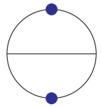
Figure 8: The unique vacuum integral topology capturing the UV properties of the analytically-continued $\beta$-dependent double-trace terms in the two-gluon two-scalar amplitude.

Using the symmetries of the numerator factors listed in eqs. (101)-(112) and (117)-(123) and momentum conservation, the coefficients of this vacuum integral in the two scalar functions are as follows:

$$M_{14;23}^{\beta,(2)}: 2\beta_{4}+2\beta_{5}+2\gamma_{3}+2\gamma_{4}=0$$ (127)

$$M_{13;24}^{\beta,(2)}: 2\beta^{\prime}_{2}+2\beta^{\prime}_{3}+4\rho^{\prime}_{1}+4\eta^{\prime}_{1}=0\ .$$ (128)

This cancellation implies that the analytic continuation of the leading $\beta$-dependent correction to the two-gluon two-scalar amplitude is finite in $D=5$; Lorentz invariance implies then that this amplitude first diverges in

$$D_{c}=6\ .$$ (129)

Even though the $\beta$-deformed theory has only ${\cal N}=1$ supersymmetry, as discussed in the introduction, this critical formal dimension is characteristic to a finite ${\cal N}=2$ theory. In a strict four-dimensional formulation, our result is that the degree of divergence is $\omega=-4$, which is smaller by two units than the expected degree of divergence of a finite ${\cal N}=1$ theory, $\omega=-2$.

7 Summary and further comments

In this paper we discussed in detail the scattering amplitudes of the $\beta$-deformed ${\cal N}=4$ sYM theory at the nonplanar level though two loops. The existence of double-trace components of tree-level amplitudes makes the scattering matrix of this theory unconstrained by the general analysis of [6]; these terms, directly linked to the existence of symmetric structure constant couplings as well as to the non-decoupling of chiral multiplets charged under the diagonal $U(1)$ subgroup of the gauge group, play an important role in the finiteness of the theory.

We have seen that, apart from planar structures inherited from the ${\cal N}=4$ theory due to the structure of the deformation, certain non-planar color structures are also protected from being directly affected by the deformation, to all orders in perturbation theory. These amplitudes may nevertheless depend on the deformation parameter through the coefficient of the superpotential whose value is fixed in terms of $\beta$, $N$ and the gauge coupling by the requirement of conformal invariance. We have also discussed the loop order at which the known expression for this coefficient requires further corrections. We identified a simple color-based argument which recovers the form of its one-loop expression and the fact that it also implies that the theory is finite at two-loop level. The same argument implies that the next correction is required at three-loop level. The existence of a superpotential coefficient leading to an all-order finiteness for the $\beta$-deformed theory is guaranteed by the original argument of Leigh and Strassler [7]. It should be interesting to find an all-order closed-form expression for this coefficient.

By explicitly evaluating four-point loop amplitudes we found that, while at one-loop level the UV properties of the theory can be explained by its ${\cal N}=1$ supersymmetry, some two-loop amplitudes exhibit an improved behavior. It is not clear what is the origin of this improvement. It is however interesting to notice its similarity with the improved UV behavior of the double-trace terms in the ${\cal N}=4$ sYM theory. In that case, a supersymmetry-based explanation of this phenomenon was identified in [62]. While we do not understand the fundamental origin of our result, an argument similar to that of [62] does not appear possible in our case. Another explanation of the ${\cal N}=4$ improved double-trace behavior was suggested in [3], essentially based on the structure of the amplitude required by color/kinematics duality. These arguments do not appear to extend in a straightforward way to the $\beta$-deformed theory due to its different color structure.

We are therefore led to suggest that the improved UV properties of the double-trace terms in both the $\beta$-deformed and in the ${\cal N}=4$ sYM theory must have yet a different explanation, common to both theories, which does not rely either on supersymmetry or on color/kinematics duality. This also points to further hidden structure in the non-planar ${\cal N}=4$ theory.

Naive inspection of the one- and two-loop amplitudes found in § 4 and § 5 does not reveal obvious consequences of the numerator relations inherited from the color/kinematics duality of the undeformed theory. It is nevertheless possible that loop amplitudes are affected – and perhaps constrained – by these tree-level numerator relations. It would be interesting to identify these consequences. In a similar direction, the main obstacle for the existence of a full-fledged color/kinematics duality in the $\beta$-deformed theory is the appearance of symmetric structure constants. The arguments of Leigh and Strassler suggest that it should not be possible to forbid their appearance without breaking conformal invariance at the quantum level. There may exist theories which, while exhibiting BCJ duality, also share some of the planar properties of the ${\cal N}=4$ theory. Identifying and studying such theories may shed further light on the relations between the symmetries of the ${\cal N}=4$ theory, the possible patterns in which they can be broken and may also expose other unexpected features which are hidden by the large symmetry of this theory.

References

- [1] N. Arkani-Hamed, J. L. Bourjaily, F. Cachazo, S. Caron-Huot and J. Trnka, “The All-Loop Integrand for Scattering Amplitudes in Planar Sym,” JHEP 1101 (2011) 041 [arXiv:1008.2958 [hep-th]].
- [2] Z. Bern, J. J. M. Carrasco, L. J. Dixon, H. Johansson and R. Roiban, “Manifest Ultraviolet Behavior for the Three-Loop Four-Point Amplitude of Supergravity,” Phys. Rev. D 78 (2008) 105019 [arXiv:0808.4112 [hep-th]].
- [3] Z. Bern, J. J. M. Carrasco, L. J. Dixon, H. Johansson and R. Roiban, “The Complete Four-Loop Four-Point Amplitude in Super-Yang-Mills Theory,” Phys. Rev. D 82 (2010) 125040 [arXiv:1008.3327 [hep-th]].
- [4] Z. Bern, J. J. M. Carrasco, H. Johansson, “New Relations for Gauge-Theory Amplitudes,” Phys. Rev. D78, 085011 (2008). [arXiv:0805.3993 [hep-ph]].
- [5] R. Monteiro and D. O’Connell, “The Kinematic Algebra from the Self-Dual Sector,” JHEP 1107 (2011) 007 [arXiv:1105.2565 [hep-th]].
- [6] P. Benincasa and F. Cachazo, “Consistency Conditions on the S-Matrix of Massless Particles,” arXiv:0705.4305 [hep-th].
- [7] R. G. Leigh, M. J. Strassler, “Exactly marginal operators and duality in four-dimensional N=1 supersymmetric gauge theory,” Nucl. Phys. B447, 95-136 (1995). [hep-th/9503121].
- [8] V. VKhoze, “Amplitudes in the beta-deformed conformal Yang-Mills,” JHEP 0602, 040 (2006). [hep-th/0512194].
- [9] N. Beisert and R. Roiban, “Beauty and the Twist: the Bethe Ansatz for Twisted Sym,” JHEP 0508 (2005) 039 [arXiv:hep-th/0505187].
- [10] S. Frolov, “Lax Pair for Strings in Lunin-Maldacena Background,” JHEP 0505 (2005) 069 [arXiv:hep-th/0503201].
- [11] O. Lunin, J. M. Maldacena, “Deforming field theories with U(1) x U(1) global symmetry and their gravity duals,” JHEP 0505, 033 (2005). [hep-th/0502086].
- [12] N. Berkovits and J. Maldacena, “Fermionic T-Duality, Dual Superconformal Symmetry, and the Amplitude/Wilson Loop Connection,” JHEP 0809 (2008) 062 [arXiv:0807.3196 [hep-th]].
- [13] N. Beisert, R. Ricci, A. A. Tseytlin and M. Wolf, “Dual Superconformal Symmetry from AdS5 S5 Superstring Integrability,” Phys. Rev. D 78 (2008) 126004 [arXiv:0807.3228 [hep-th]].
- [14] L. F. Alday, J. M. Henn, J. Plefka and T. Schuster, “Scattering into the Fifth Dimension of Super Yang-Mills,” JHEP 1001 (2010) 077 [arXiv:0908.0684 [hep-th]].
- [15] T. Filk, “Divergencies in a field theory on quantum space,” Phys. Lett. B376, 53-58 (1996).
- [16] F. Elmetti, A. Mauri, S. Penati and A. Santambrogio, “Conformal Invariance of the Planar Beta-Deformed Sym Theory Requires Beta Real,” JHEP 0701 (2007) 026 [arXiv:hep-th/0606125].
- [17] A. Dymarsky, R. Roiban, unpublished
- [18] D. Z. Freedman and U. Gursoy, “Comments on the beta-deformed N = 4 SYM theory,” JHEP 0511, 042 (2005) [arXiv:hep-th/0506128].
- [19] S. Penati, A. Santambrogio and D. Zanon, “Two-point correlators in the beta-deformed N = 4 SYM at the next-to-leading order,” JHEP 0510, 023 (2005) [arXiv:hep-th/0506150].
- [20] N. Dorey, “S duality, deconstruction and confinement for a marginal deformation of N=4 SUSY Yang-Mills,” JHEP 0408, 043 (2004). [hep-th/0310117].
- [21] N. Dorey, T. J. Hollowood, “On the Coulomb branch of a marginal deformation of N = 4 SUSY Yang-Mills,” JHEP 0506, 036 (2005). [hep-th/0411163].
- [22] S. M. Kuzenko, I. N. McArthur, “Effective action of beta-deformed N = 4 SYM theory: Farewell to two-loop BPS diagrams,” Nucl. Phys. B778, 159-191 (2007). [hep-th/0703126 [HEP-TH]].
- [23] R. Akhoury, “Mass Divergence of Wide Angle Scattering Amplitudes”, Phys. Rev. D19, 1250 (1979).
- [24] A. H. Mueller, “On the Asymptotic Behavior of the Sudakov Form-factor”, Phys. Rev. D20, 2037 (1979).
- [25] J. C. Collins, “Algorithm to Compute Corrections to the Sudakov Form-factor”, Phys. Rev. D22, 1478 (1980).
- [26] A. Sen, “Asymptotic Behavior of the Sudakov Form-Factor in QCD”, Phys. Rev. D24, 3281 (1981).
- [27] G. Sterman, “Summation of Large Corrections to Short Distance Hadronic Cross-Sections”, Nucl. Phys. B281, 310 (1987).
- [28] J. Botts and G. Sterman, “Sudakov Effects in Hadron Hadron Elastic Scattering”, Phys. Lett. B224, 201 (1989).
- [29] S. Catani and L. Trentadue, “Resummation of the QCD Perturbative Series for Hard Processes”, Nucl. Phys. B327, 323 (1989).
- [30] G. P. Korchemsky, “Sudakov Form-factor in QCD”, Phys. Lett. B220, 629 (1989).
- [31] L. Magnea and G. Sterman, “Analytic continuation of the Sudakov form-factor in QCD”, Phys. Rev. D42, 4222 (1990).
- [32] G. P. Korchemsky and G. Marchesini, “Resummation of large infrared corrections using Wilson loops”, Phys. Lett. B313, 433 (1993).
- [33] S. Catani, “The singular behaviour of QCD amplitudes at two-loop order”, Phys. Lett. B427, 161 (1998), hep-ph/9802439.
- [34] G. Sterman and M. E. Tejeda-Yeomans, “Multi-loop amplitudes and resummation”, Phys. Lett. B552, 48 (2003), hep-ph/0210130.
- [35] J. C. Collins, D. E. Soper and G. Sterman, “Factorization of Hard Processes in QCD”, Adv. Ser. Direct. High Energy Phys. 5, 1 (1988), hep-ph/0409313.
- [36] A. Sen, “Asymptotic Behavior of the Wide Angle On-Shell Quark Scattering Amplitudes in Nonabelian Gauge Theories”, Phys. Rev. D28, 860 (1983).
- [37] S. M. Aybat, L. J. Dixon and G. Sterman, “The two-loop soft anomalous dimension matrix and resummation at next-to-next-to leading pole”, Phys. Rev. D74, 074004 (2006), hep-ph/0607309.
- [38] A. Mauri, S. Penati, A. Santambrogio and D. Zanon, “Exact Results in Planar Superconformal Yang-Mills Theory,” JHEP 0511 (2005) 024 [arXiv:hep-th/0507282].
- [39] S. Ananth, S. Kovacs and H. Shimada, “Proof of All-Order Finiteness for Planar Beta-Deformed Yang-Mills,” JHEP 0701 (2007) 046 [arXiv:hep-th/0609149].
- [40] Z. Bern, D. A. Kosower, “Color decomposition of one loop amplitudes in gauge theories,” Nucl. Phys. B362, 389-448 (1991).
- [41] V. Del Duca, L. J. Dixon and F. Maltoni, “New Color Decompositions for Gauge Amplitudes at Tree and Loop Level,” Nucl. Phys. B 571 (2000) 51 [arXiv:hep-ph/9910563].
- [42] Z. Bern, L. J. Dixon, D. C. Dunbar and D. A. Kosower, “One-Loop N-Point Gauge Theory Amplitudes, Unitarity and Collinear Limits,” Nucl. Phys. B 425 (1994) 217 [arXiv:hep-ph/9403226].
- [43] Z. Bern, L. J. Dixon, D. C. Dunbar and D. A. Kosower, “Fusing Gauge Theory Tree Amplitudes into Loop Amplitudes,” Nucl. Phys. B 435 (1995) 59 [arXiv:hep-ph/9409265].
- [44] Z. Bern, L. J. Dixon and D. A. Kosower, “One-Loop Amplitudes for E+ E- to Four Partons,” Nucl. Phys. B 513 (1998) 3 [arXiv:hep-ph/9708239].
- [45] R. Britto, F. Cachazo and B. Feng, “Generalized Unitarity and One-Loop Amplitudes in Super-Yang-Mills,” Nucl. Phys. B 725 (2005) 275 [arXiv:hep-th/0412103].
- [46] E. I. Buchbinder and F. Cachazo, “Two-Loop Amplitudes of Gluons and Octa-Cuts in Super Yang-Mills,” JHEP 0511 (2005) 036 [arXiv:hep-th/0506126].
- [47] Z. Bern, J. J. M. Carrasco, H. Ita, H. Johansson and R. Roiban, “On the Structure of Supersymmetric Sums in Multi-Loop Unitarity Cuts,” Phys. Rev. D 80 (2009) 065029 [arXiv:0903.5348 [hep-th]].
- [48] H. Elvang, Y. t. Huang and C. Peng, “On-Shell Superamplitudes in N¡4 Sym,” JHEP 1109 (2011) 031 [arXiv:1102.4843 [hep-th]].
- [49] Z. Bern, L. J. Dixon, D. C. Dunbar and D. A. Kosower, Phys. Lett. B 394, 105 (1997) [hep-th/9611127].
- [50] L. F. Alday and J. M. Maldacena, “Gluon Scattering Amplitudes at Strong Coupling,” JHEP 0706 (2007) 064 [arXiv:0705.0303 [hep-th]].
- [51] M.T. Grisaru, H.N. Pendleton and P. van Nieuwenhuizen, Phys. Rev. D15:996 (1977); M.T. Grisaru and H.N. Pendleton, Nucl. Phys. B124:81 (1977); S.J. Parke and T. Taylor, Phys. Lett. 157B:81 (1985).
- [52] I. Chepelev, R. Roiban, “Renormalization of quantum field theories on noncommutative R**d. 1. Scalars,” JHEP 0005, 037 (2000). [hep-th/9911098].
- [53] R. Britto, E. Buchbinder, F. Cachazo and B. Feng, “One-Loop Amplitudes of Gluons in Sqcd,” Phys. Rev. D 72 (2005) 065012 [arXiv:hep-ph/0503132].
- [54] M. B. Green, J. H. Schwarz, L. Brink, Nucl. Phys. B198, 474-492 (1982).
- [55] Z. Bern, L. J. Dixon and D. A. Kosower, “Dimensionally Regulated Pentagon Integrals,” Nucl. Phys. B 412 (1994) 751 [arXiv:hep-ph/9306240].
- [56] P. S. Howe and K. S. Stelle, “Supersymmetry Counterterms Revisited,” Phys. Lett. B 554 (2003) 190 [arXiv:hep-th/0211279].
- [57] V. A. Smirnov and O. L. Veretin, “Analytical results for dimensionally regularized massless on-shell double boxes with arbitrary indices and numerators,” Nucl. Phys. B 566, 469 (2000) [hep-ph/9907385].
- [58] Z. Bern, L. J. Dixon, D. C. Dunbar, M. Perelstein and J. S. Rozowsky, “On the Relationship Between Yang-Mills Theory and Gravity and Its Implication for Ultraviolet Divergences,” Nucl. Phys. B 530 (1998) 401 [arXiv:hep-th/9802162].
- [59] Z. Bern, J. J. Carrasco, L. J. Dixon, H. Johansson, D. A. Kosower and R. Roiban, “Three-Loop Superfiniteness of N=8 Supergravity,” Phys. Rev. Lett. 98, 161303 (2007) [hep-th/0702112].
- [60] Z. Bern, J. J. Carrasco, L. J. Dixon, H. Johansson and R. Roiban, “The Ultraviolet Behavior of N=8 Supergravity at Four Loops,” Phys. Rev. Lett. 103, 081301 (2009) [0905.2326 [hep-th]].
- [61] N. Marcus and A. Sagnotti, “A Simple Method For Calculating Counterterms,” Nuovo Cim. A 87, 1 (1985).
- [62] N. Berkovits, M. B. Green, J. G. Russo and P. Vanhove, “Non-Renormalization Conditions for Four-Gluon Scattering in Supersymmetric String and Field Theory,” JHEP 0911 (2009) 063 [arXiv:0908.1923 [hep-th]].