Currents in complex polymers: an example of superstatistics for short time series

Abstract

We apply superstatistical techniques to an experimental time series of measured transient currents through a thin Aluminium-PMMA-Aluminium film. We show that in good approximation the current can be approximated by local Gaussian processes with fluctuating variance. The marginal density exhibits ’fat tails’ and is well modelled by a superstatistical model. Our techniques can be generally be applied to other short time series as well.

I Introduction

Many time series generated by complex systems in nature are superstatistical, i.e they consist of a superposition of several dynamics on well-separated time scales. Often, there is locally a simple dynamics (for example, a Gaussian process) and the parameters of that simple process fluctuate on a much larger scale. Such varying parameters describe a changing environment of the local system under consideration. Often the relevant measured time series consists locally of a Gaussian process, with the variance of those Gaussians evolving on a longer time scale. In nonequilibrium statistical mechanics, the technique of superstatistics was introduced in beck-cohen and has since then provided a powerful tool to describe a large variety of complex systems for which there is change of environmental conditions swinney ; touchette ; souza ; chavanis ; jizba ; frank ; celia ; straeten . A superstatistical complex system is mathematically described as a multi-scale superposition of two (or several) statistics, one corresponding to local equilibrium statistical mechanics (on a mesoscopic level modeled by a linear Langevin equation leading to locally Gaussian behavior) and the other one corresponding to a slowly varying parameter $a$ of the system. Essential for this approach is the fact that there is sufficient time scale separation, i.e. the local relaxation time of the system must be much shorter than the typical time scale on which the parameter $a$ changes. There is interesting mathematics associated with superstatistical complex systems. For example, in a recent paper hanel Hanel, Thurner and Gell-Mann showed that the superstatistical distribution function $f(a)$ cannot change in an arbitrary way under macroscopic state changes of the system, and that the underlying transformation group is the Euclidean group in 1 dimension.

In most applications in nonequilibrium statistical mechanics the slowly varying control parameter $a$, underlying the superstatistical dynamics, is the local inverse temperature $\beta$ of the system, i.e. $a=\beta$. However, in general the control parameter $a$ can also have a different meaning. For example in mathematical finance, $a$ is a vooatility parameter describing changing market behavior and turbulences in the market. For a time series, $a$ is usually a local variance parameter that can be directly extracted from suitably chosen time slices. There are numerous interesting applications of the superstatistics concept to real-world problems, for example to train delay statisticsbriggs , hydrodynamic turbulence prl and cancer survival statistics chen . For further applications, see daniels ; maya ; reynolds ; abul-magd ; rapisarda ; cosmic .

In this paper, we apply for the first time superstatistical techniques to a complex systems of solid state physics. We are interested in the statistical properties of currents flowing through thin films when a voltage is applied. Our measured system is a thin aluminium-polymethylmethacrylate-aluminium film (Al-PMMA-Al). A detailed experimental investigation of this system was presented in hacinliyan2003 ; hacinliyan2006 . A particular feature of this system is that when a voltage is applied, the corresponding measured currents exhibit transient (nonstationary) behavior with strong fluctuations. This can be formally associated with transient chaotic behavior, and in the above papers formally a small positive Liapunov exponent was extracted from the data. More recently, Yalcin et al singapore ; yalcin made a statistical analysis of the fluctuating current data using $q$-statistics, inspired by the fact that $q$-statistics europhysics is often used for weakly chaotic systems which have approximately zero Lyapunov exponent miritello ; alessandro ; tsallis-book .

In this paper we show that the measured current data can be well modelled by a superstatistical dynamics. However, in contrast to previous superstatistical time series analysis techniques described in straeten , one has a typical problem for these kinds of data: The time series is not long enough to apply the standard superstatistical techniques developed in straeten . Still, in this paper we show what one can typically do for a short time series. Our method described in the following is quite simple and general and can be applied to other small data sets in a similar way.

II Analyzing the experimental time series

Figs. 1-3 show typical time series of increments $I(t)=i(t+1)-i(t)$ of the measured current $i(t)$ through the Al-PMMA-Al film at three different temperatures. The average value has been substracted, and all data are rescaled by dividing through the standard deviation $\sigma$ determined from the entire time series. We define $u(t)=(I(t)-\langle I(t)\rangle)/\sigma$.

One clearly observes regions of strong activity interwoven with periods of much calmer behavior, similar as for turbulent flows of share price evolution data. To analyse these data, we divide the time series into a couple of windows with qualitatively similar behavior. These windows are shown as vertical lines in Fig.1-3.

 

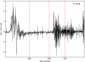
Figure 1: The current magnitude differences $I(t)=i(t+1)-i(t)$ for the transient current through thin Al-PMMA-Al film at $T=295K$ yalcin

 

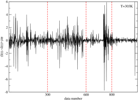
Figure 2: The current magnitude differences $I(t)=i(t+1)-i(t)$ for the transient current through thin Al-PMMA-Al film at $T=303K$

 

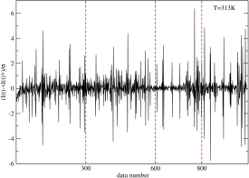
Figure 3: The current magnitude differences $I(t)=i(t+1)-i(t)$ for the transient current through thin Al-PMMA-Al film at $T=313K$

 

The choice of the windows is rather arbitrary, they should be large enough to contain enough statistics, but still be significantly shorter than the entire time series.

For each local window, we look at a histogram of the fluctuating currents. As shown in Fig. 4-7, locally the behavior is well approximated by a Gaussian distribution

$$p(u|\beta)=\sqrt{\frac{\beta}{2\pi}}exp\left\{-\frac{1}{2}\beta u^{2}\right\}$$ (1)

However, the local variance parameter $\beta$ varies strongly from window to window and is thus itself a random variable, as expected for superstatistical systems.

 

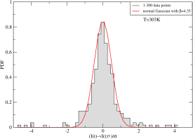
Figure 4: Gaussian fit to the observed local probability density for data points 1-300 of the measured time series of current differences $I(t)$ at $T=303K$.

 

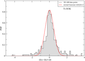
Figure 5: Same as Fig. 4 for data points 301-600 of the measured time series

 

 

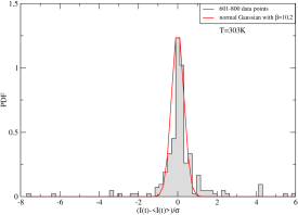
Figure 6: Same as Fig. 4 for data points 601-800 of the measured time series

 

 

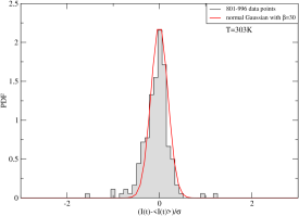
Figure 7: Same as Fig. 4 for data points 801-996 of the measured time series

Tab. 1 shows the values of extracted variance parameters $\beta_{i}$ for the various windows and for different temperatures $T$ where the experiment was performed.

We can only extract a few values $\beta_{i}$ from our short time series. The general idea of superstatistics is that the marginal distribution $p(u)$ is given as a superposition

$$p(u)=\int f(\beta)p(u|\beta)d\beta$$ (2)

for a suitable $f(\beta)$ describing the distribution of $\beta$-values. For a short time series, as in our case, one can only make guesses of the relevant $f(\beta)$. For this it is useful to look at the histogram of the entire time series, sampling up the behavior in all windows. This is shown in Fig. 8.

 

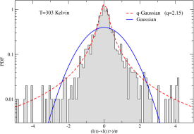
Figure 8: Entire PDF of the current magnitude differences $I(t)=i(t+1)-i(t)$ for the transient current through thin Al-PMMA-Al at temperature $T=303K$  yalcin

Apparently, the histogram data of the entire time series are well-fitted by $q$-Gaussians of the form

$$p(u)\sim(1+\frac{1}{2}\tilde{\beta}(q-1)u^{2})^{\frac{1}{1-q}}.$$ (3)

The corresponding parameters $\tilde{\beta}$ and $q$ are shown in Tab.1.

	$\beta_{1}$	$\beta_{2}$	$\beta_{3}$	$\beta_{4}$	$\beta_{0}$	$\tilde{\beta}$	$q$
T=295K	4.9	66	8.8	8.1	21.95	40	2.3
T=303K	4.35	4.2	10.2	30	12.1875	30	2.15
T=313K	4	6.95	18.5	6.2	8.9125	22	2.1

Table 1: The values of extracted variance parameters $\beta_{1}$, $\beta_{2}$, $\beta_{3}$, $\beta_{4}$,and $\beta_{0}$ for the various slices, for the measured current through thin Al-PMMA-Al film at temperature $T=295,~{}303~{}and~{}313K$. Also shown $q$ and $\tilde{\beta}$.

We cannot, as for longer time series straeten , extract the relevant distribution $f(\beta)$ from a histogram of $\beta_{i}$-values, since there are only 4 data points. But the fitting result (3) can be used to theoretically predict $f(\beta)$. In our case $f(\beta)$ is in good approximation a $\chi^{2}$ (or $\Gamma$)-distribution, meaning that if we were able to look at much longer time series, then the $\beta_{i}$ would be distributed according to

$$f(\beta)=\frac{1}{\Gamma(\frac{n}{2})}\left\{\frac{n}{2\beta_{0}}\right\}^{n/2}\beta^{n/2-1}exp\left\{-\frac{n\beta}{2\beta_{0}}\right\}$$ (4)

This follows from doing the integral (2) using the distribution (4), which directly leads to the observed fitting result (3). The relation between the parameters $n$ and $q$ is prl2001

$$q=1+\frac{2}{n+1}.$$ (5)

Moreover, the parameter $\tilde{\beta}$ is related to the average value of $\beta$ by prl2001

$$\beta_{0}:=\int f(\beta)\beta d\beta=\frac{(3-q)}{2}\tilde{\beta}$$ (6)

The predicted superstatistical distributions $f(\beta)$ are plotted in Fig. 9 for the three different temperatures. We can also calculate the average value of $\beta_{0}$ directly from the time series, namely from the values $\beta_{i}$ fitted in the 4 windows, i.e. $\beta_{0}=\frac{1}{4}(\beta_{1}+\beta_{2}+\beta_{3}+\beta_{4})$. The result is shown in Tab. 1 as well. This sum has huge error terms, because only 4 windows enter, and the partioning into windows is rather arbitrary. Nevertheless, the obtained average values are consistent with the theoretically predicted result (6) within the statistical error bounds.

 

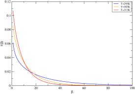
Figure 9: $f(\beta)$ of the measured time series through Al-PMMA-Al film at temperature $T=295,~{}303~{}and~{}313K$

To summarize, for very long time series, one has theoretical methods to decide whether a given time series is superstatistical or not straeten . For short time series, as in our case, these methods are not applicable. Still one can do the method proposed in the current paper quite generally. First one looks whether a partitioning into a few windows is possible such that locally Gaussian behavior is observed. Then one determines the local variance parameters $\beta_{i}$. From a histogram of the entire time series one obtains a guess what the relevant distribution $f(\beta)$ could be—in our case a $\chi^{2}$-distribution but in general these can be other distributions such as e.g. the lognormal or inverse-$\chi^{2}$ distribution swinney . After that guess, one can check consistency of derived parameter relations within the statistical error bounds, in our case given by relation (6) but in general given by other relations, depending on $f(\beta)$.

III Acknowledgement

G.C.Y. was supported by the Scientific Research Projects Coordination Unit of Istanbul University with project number 7441. G.C.Y gratefully acknowledges the hospitality of Queen Mary University of London, School of Mathematical Sciences, where this work was carried out. G.C.Y and C.B. would like to thank Prof. Murray Gell-Mann for useful discussions on the subject.

References

- (1) C. Beck and E.G.D. Cohen, Physica A 322, 267 (2003)
- (2) C. Beck, E.G.D. Cohen, and H.L. Swinney,Phys. Rev. E 72, 056133 (2005)
- (3) H. Touchette and C. Beck, Phys. Rev. E 71, 016131 (2005)
- (4) C. Tsallis and A.M.C. Souza, Phys. Rev. E 67, 026106 (2003)
- (5) P. Jizba, H. Kleinert, Phys. Rev. E 78, 031122 (2008)
- (6) P.-H. Chavanis, Physica A 359, 177 (2006)
- (7) S.A. Frank and D.E. Smith, Entropy 12, 289 (2010)
- (8) C. Anteneodo and S.M. Duarte Queiros, J. Stat. Mech. P10023 (2009)
- (9) E. Van der Straeten and C. Beck, Phys. Rev. E 80, 036108 (2009)
- (10) R. Hanel, S. Thurner, and M. Gell-Mann, PNAS 108, 6390 (2011)
- (11) K. Briggs, C. Beck, Physica A 378, 498 (2007)
- (12) C. Beck, Phys. Rev. Lett. 98, 064502 (2007)
- (13) L. Leon Chen, C. Beck, Physica A 387, 3162 (2008)
- (14) A.Y. Abul-Magd, G. Akemann, P. Vivo, J. Phys. A Math. Theor. 42, 175207 (2009)
- (15) K.E. Daniels, C. Beck, and E. Bodenschatz, Physica D 193, 208 (2004)
- (16) C. Beck, Physica A 331, 173 (2004)
- (17) M. Baiesi, M. Paczuski and A.L. Stella, Phys. Rev. Lett. 96, 051103 (2006)
- (18) S. Rizzo and A. Rapisarda, AIP Conf. Proc. 742, 176 (2004)
- (19) A. Reynolds, Phys. Rev. Lett. 91, 084503 (2003)
- (20) A. Hacinliyan, Y. Skarlatos, G. Sahin and G. Akin, Chaos Solitons Fractals 17, 575-583 (2003)
- (21) A. Hacinliyan, Y. Skarlatos, H.A. Yildirim and G. Sahin, Fractals 14, 125-131 (2006)
- (22) G.C. Yalcin, Y. Skarlatos and K.G. Akdeniz, in Proceedings of the Conference in Honour of Murray Gell-Mann’s 80th Birthday Quantum Mechanics, Elementary Particles, Quantum Cosmology and Complexity , Singapore, 2010, edited by H.Fritzsch and K.K.Phu (World Scientific Publishing, Singapore, 2010, ISBN:978-981-4335-60-7), p.669
- (23) G.C.Yalcin,Y.Skarlatos, and K.G.Akdeniz, Istanbul University, Physics Department Preprint (July,2011)
- (24) C. Tsallis, M. Gell-Mann and Y. Sato, Europhy. News 36, 186-189 (2005)
- (25) G. Miritello, A. Pluchino and A. Rapisarda, Phys. A 388, 4818-4826 (2009)
- (26) F. Caruso, A. Pluchino, V. Latora, S. Vinciguerra and A. Rapisarda, Phys. Rev. E 75, 055101-4 (2007)
- (27) C. Tsallis, Introduction to Nonextensive Statistical Mechanics, Springer, 2009
- (28) C. Beck, Phys. Rev. Lett. 87, 180601 (2001)