Multimode solutions of first-order elliptic quasilinear systems obtained from Riemann invariants

Abstract

Two new approaches to solving first-order quasilinear elliptic systems of PDEs in many dimensions are proposed. The first method is based on an analysis of multimode solutions expressible in terms of Riemann invariants, based on links between two techniques, that of the symmetry reduction method and of the generalized method of characteristics. A variant of the conditional symmetry method for constructing this type of solution is proposed. A specific feature of that approach is an algebraic-geometric point of view, which allows the introduction of specific first-order side conditions consistent with the original system of PDEs, leading to a generalization of the Riemann invariant method for solving elliptic homogeneous systems of PDEs. A further generalization of the Riemann invariants method to the case of inhomogeneous systems, based on the introduction of specific rotation matrices, enables us to weaken the integrability condition. It allows us to establish a connection between the structure of the set of integral elements and the possibility of constructing specific classes of simple mode solutions. These theoretical considerations are illustrated by the examples of an ideal plastic flow in its elliptic region and a system describing a nonlinear interaction of waves and particles. Several new classes of solutions are obtained in explicit form, including the general integral for the latter system of equations.

Keywords:symmetry reduction method, generalized method of characteristics, Riemann invariants, multimode solutions Mathematics Subject Classification (2000): 35B06; 35F50; 35F20

I Introduction

Riemann waves represent a very important class of solutions of nonlinear first-order systems of partial differential equations (PDEs). They are ubiquitous in the differential equations of mathematical physics, since they appear in all multidimensional hyperbolic systems and constitute their elementary solutions. Their characteristic feature is that, in most cases, they are expressible only in implicit form. For a homogeneous hyperbolic quasilinear system of first-order PDEs,

$$\mathcal{A}_{\alpha}^{i\mu}(u)\frac{\partial u^{\alpha}}{\partial x^{i}}=0,\qquad i=1,\ldots,p,\quad\alpha=1,\ldots,q,\quad\mu=1,\ldots,m$$ (1)

(where $\mathcal{A}^{1},\ldots,\mathcal{A}^{p}$ are $q\times m$ matrix functions of an unknown function $u$ and we adopt the convention that repeated indices are summed), a Riemann wave solution is defined by the equation $u=f(r(x,u))$, where $f\colon\mathbb{R}\rightarrow\mathbb{R}^{q}$, and the function $r(x,u)=\lambda_{i}(u)x^{i}$ is called the Riemann invariant associated with the vector $\lambda$. This vector $\lambda$ satisfies the equation $\ker\left(\lambda_{i}\mathcal{A}^{i}(u)\right)\neq 0$. Such Riemann wave solutions have rank at most equal to one. They are building blocks for the construction of more general types of solutions describing nonlinear superpositions of many waves ($k$-waves), which are very interesting from the physical point of view.

Until now, the only way to approach this task was through the generalized method of characteristics (GMC) (see e.g. [3, 7, 22, 23, 33, 34]) and more recently through the conditional symmetry method (CSM) [1, 6, 13, 14, 15, 32]. The GMC relies on treating Riemann invariants as new dependent variables (which remain constant along the appropriate characteristic curves of the initial system (1) and constitute a set of invariants of the Abelian algebra of some vector field $X_{a}=\xi_{a}^{i}(u)\partial_{x}^{i}$ with $\lambda_{i}^{a}\xi_{a}^{i}=0$ for $1\leq a\leq k<p$. This leads to a reduction of the dimension of the problem. The most important theoretical results obtained with the use of the GMC or CSM [15] include the necessary and sufficient conditions for the existence of Riemann $k$-waves in multidimensional systems. It was shown [33] that these solutions depend on $k$ arbitrary functions of one variable. Some criteria were also found [33] for determining the elastic or nonelastic character of the superposition of Riemann waves described by hyperbolic systems, which is particularly useful in physical applications. In applications to fluid dynamics and nonlinear field theory, many new and interesting results were obtained [2, 3, 10, 11, 12, 23, 30, 34, 36, 37].

Both the GMC and CSM methods, like all other techniques for solving PDEs, have their limitations. This fact has motivated the authors to search for the means of constructing larger classes of multiple wave solutions expressible in terms of Riemann invariants by allowing the introduction of complex integral elements in the place of real simple integral elements (with which the solutions of hyperbolic systems are built [33]). This idea originated from the work of S. Sobolev [35] in which he solves the wave equation by using the associated complex wave vectors. We are particularly interested in the construction of nonlinear superpositions of elementary simple mode solutions, and the proposed analysis indicates that the language of conditional symmetries is an effective tool for this purpose. This approach is applied to the nonstationary irrotational flow of an ideal plastic material in its elliptic region. A further extension of the proposed method to the case of inhomogeneous systems is proposed in order to be applicable either in the elliptic or hyperbolic regions. This allows for a wider range of physical applications. The approach is based on the use of rotation matrices which obey certain algebraic conditions and allow us to write the reduced system in terms of Riemann invariants in the sense that each derivative of a dependent variable is equal to an algebraic expression (see equation (87)). We discuss in detail the sufficient conditions for the existence of multimode solutions. This approach is applied to a system describing the propagation of shock waves in the nonlinear interaction of waves and particles. The general integral of this system has been constructed in explicit form depending on two arbitrary functions of one variable. Through this paper, all derivatives, transformations, surfaces and solutions are assumed to be local.

The organization of this paper is as follows. Section II contains a detailed account of the generalized method of characteristics for first-order quasilinear systems of PDEs in many dimensions based on complex characteristic elements. In Section III we formulate the problem of multimode solutions expressible in terms of Riemann invariants by means of a group theoretical approach. This allows us to formulate the necessary and sufficient conditions for constructing these types of solutions. In Section C, the usefulness of the method developed in Section III is illustrated by the example of ideal plasticity in $(2+1)$ dimensions, in which we find several bounded solutions. Moreover, we have drawn extrusion dies and the flow inside them (limiting ourselves to the region where the gradient catastrophe does not occur). Sections IV and V comprise a new approach to solving inhomogeneous elliptic systems in order to obtain simple wave and simple mode solutions. In Section VI, we show an example of a simple mode solution, obtained through the method presented in Section V. The technique is applied to a system describing the propagation of shock waves and the nonlinear interaction of waves and particles. We obtain its general solution. Section VII summarizes the results obtained and contains some suggestions regarding further developments.

II The method of characteristics for complex integral elements

The methodological approach assumed in this section is based on a generalized method of characteristics which has been extensively developed (see e.g. [3, 9, 16, 19, 33] and references therein) for multidimensional homogeneous and inhomogeneous systems of first-order PDEs. A specific feature of that approach is that it has both an algebraic and geometric point of view. An algebraization of systems of PDEs is made possible by representing the general integral elements as linear combinations of some special elements associated with those vector fields which generate characteristic curves in the spaces of independent variables $X$ and dependent variables $U$, respectively (see e.g. [18, 33]). The introduction of these elements (called simple integral elements) turns out to be very useful for the construction of certain classes of rank-$k$ solutions in closed form. These integral elements correspond to Riemann wave solutions in the case of nonelliptic systems and serve to construct multiple waves ($k$-waves) as superpositions of several single Riemann waves.

The generalized method of characteristics for solving quasilinear hyperbolic first-order systems can be extended to the case of complex characteristic elements (see e.g. [33, 35]). These elements, which had originally been introduced for hyperbolic systems, were generalized to the case of elliptic systems by allowing the wave vectors to be the complex solutions of the dispersion relation associated with the initial system of equations. We begin by making an algebraization, according to [3, 19, 33], of a first-order system of PDEs (1) in $p$ independent and $q$ dependent variables written in the matrix form

$$\mathcal{A}^{i}(u)u_{i}=0,\quad i=1,\ldots,p,$$ (2)

$$x=(x^{1},\ldots,x^{p})\in X\subseteq\mathbb{R}^{p},\ u=(u^{1},\ldots,u^{q})\in U\subseteq\mathbb{R}^{q},$$

where $\mathcal{A}^{i}(u)=\left(\mathcal{A}^{\mu i}_{\alpha}(u)\right)$ are $m\times q$ matrix functions of $u$ and we denote the partial derivatives by $u^{\alpha}_{i}=\partial u^{\alpha}/\partial x^{i}$. The matrix $L_{i}^{\alpha}$ satisfying the conditions [3]

$$u_{i}^{\alpha}\in\left\{L_{i}^{\alpha}:\mathcal{A}_{\alpha}^{\mu i}L_{i}^{\alpha}=0,\ \mu=1,\ldots,q\right\}$$ (3)

on some open neighborhood of a given point $\tilde{u}\in U$ is called an integral element of the system (LABEL:eq:2.1). This matrix $L=\left({\partial u^{\alpha}}/{\partial x^{i}}\right)$ is a matrix of the tangent mapping $du\colon X\rightarrow T_{u}U$ given by the formula

$$X\ni(\delta x^{i})\rightarrow(\delta u^{\alpha})\in T_{u}U,\quad\text{where }\delta u^{\alpha}=u_{i}^{\alpha}\delta x^{i}.$$

The tangent mapping $du(x)$ determines an element of the linear space $L(X,T_{u}U)$, which can be identified with the tensor product $T_{u}U\otimes X^{\ast}$, (where $X^{\ast}$ is the dual space of $X$, i.e. the space of linear forms). It is well known [3, 19, 33] that each element of this tensor product can be represented as a finite sum of simple tensors of the form

$$L=\gamma\otimes\lambda,$$

where $\lambda\in X^{\ast}$ is a covector and $\gamma=\gamma^{\alpha}\frac{\partial}{\partial u^{\alpha}}\in T_{u}U$ is a tangent vector at the point $u\in U$. Hence, the integral element $L_{i}^{\alpha}$ is called a simple element if $\operatorname{rank}(L_{i}^{\alpha})=1.$ To determine a simple integral element $L_{i}^{\alpha}$ we have to find a vector field $\gamma\in T_{u}U$ and a covector $\lambda\in X^{\ast}$ satisfying the so-called wave relation

$$\left(\lambda_{i}\mathcal{A}^{\mu i}_{\alpha}(u)\right)\gamma^{\alpha}=0,\qquad\mu=1,\ldots,m.$$ (4)

The necessary and sufficient condition for the existence of a nonzero solution $\gamma$ for the equation (4) is

$$\operatorname{rank}\left(\lambda_{i}\mathcal{A}^{i}(u)\right)<q.$$ (5)

This relation is known as the dispersion relation. If the covector $\lambda=\lambda_{i}(u)dx^{i}$ satisfies the dispersion relation (5) then there exists a polarization vector $\gamma\in T_{u}U$ satisfying the wave relation (4). The algebraic approach which has been used in [3, 19, 33] for hyperbolic systems of equations (LABEL:eq:2.1) allows the construction of certain classes of $k$-wave solutions admitting $k$ arbitrary functions of one variable. The replacement of the simple real element $L_{i}^{\alpha}$ with a complex element allows us to construct more general classes of solutions. A specific form of solution $u(x)$ of the elliptic system (LABEL:eq:2.1) is postulated for which the tangent mapping $du(x)$ is a sum of a complex element and its complex conjugate

$$du^{\alpha}(x)=\xi(x)\gamma^{\alpha}(u)\lambda_{i}(u)dx^{i}+\bar{\xi}(x)\bar{\gamma}^{\alpha}(u)\bar{\lambda}_{i}(u)dx^{i},\qquad\alpha=1,\ldots,q,$$ (6)

where $\gamma=(\gamma^{1},\ldots,\gamma^{q})\in\mathbb{C}^{q}$ and $\lambda=(\lambda_{1},\ldots,\lambda_{p})\in\mathbb{C}^{p}$ satisfy

$$\lambda_{i}\mathcal{A}_{\alpha}^{\mu i}(u)\gamma^{\alpha}=0,\quad\bar{\lambda}_{i}\mathcal{A}_{\alpha}^{\mu i}(u)\bar{\gamma}^{\alpha}=0.$$ (7)

Here the quantity $\xi(x)\neq 0$ is treated as a complex function of the real variables $x$. In what follows we assume that the vectors $\gamma$ and $\bar{\gamma}$ are linearly independent. The proposed form of the solution (6) is more general than the one proposed in [22, 34] for which the derivatives $u^{\alpha}_{i}$ are represented by a real simple element leading to a simple Riemann wave solution. To distinguish this situation from the one proposed in (6), we call the real-valued solution associated with a complex element and its complex conjugate a simple mode solution in accordance with [33]. This means that all first-order derivatives of $u^{\alpha}$ with respect to $x^{i}$ are decomposable in the following way

$$\frac{\partial u^{\alpha}}{\partial x^{i}}=\xi(x)\gamma^{\alpha}(u)\lambda_{i}(u)+\bar{\xi}(x)\bar{\gamma}^{\alpha}(u)\bar{\lambda}_{i}(u),$$ (8)

where a set of functions $(\lambda,\gamma)$ and their conjugates $(\bar{\lambda},\bar{\gamma})$ on $U$ satisfy the wave relation (7). Similarly, as in the case of $k$-waves, for hyperbolic systems [33], we have to find the necessary and sufficient conditions for the existence of solutions of type (6). These conditions are called involutivity conditions.

First we derive a number of necessary conditions on the vector fields $(\gamma,\lambda)$ and their complex conjugate $(\bar{\gamma},\bar{\lambda})$ as a requirement for the existence of rank-$2$ (simple mode) solutions of the homogeneous system (LABEL:eq:2.1). Namely, closing (6) by exterior differentiation, we obtain the following 2-forms

$$\gamma\otimes(d\xi\wedge\lambda+\xi d\lambda)+\xi d\gamma\wedge\lambda+\bar{\gamma}\otimes(d\bar{\xi}\wedge\bar{\lambda}+\bar{\xi}d\bar{\lambda})+\bar{\xi}d\bar{\gamma}\wedge\bar{\lambda}=0,$$ (9)

which have to satisfy (6). Using (6) we get

$$d\lambda=\bar{\xi}\bar{\lambda}\wedge\lambda_{,\bar{\gamma}}+\xi\lambda\wedge\bar{\lambda}_{,\gamma},\qquad d\gamma=\bar{\xi}\gamma_{,\bar{\gamma}}\otimes\bar{\lambda}+\gamma_{,\lambda}\otimes d\lambda,$$ (10)

where we have used the following notation

$$\lambda_{,\gamma}=\gamma^{\alpha}\frac{\partial}{\partial u^{\alpha}}\lambda,\quad\gamma_{,\bar{\gamma}}=\bar{\gamma}^{\alpha}\frac{\partial}{\partial u^{\alpha}}\gamma.$$

Substituting (10) into the prolonged system (9) we obtain

$$\gamma\otimes\left[d\xi\wedge\lambda+\xi\bar{\xi}\bar{\lambda}\wedge\lambda_{,\bar{\gamma}}\right]+\bar{\gamma}\otimes\left[d\bar{\xi}\wedge\bar{\lambda}+\xi\bar{\xi}\lambda\wedge\bar{\lambda}_{,\gamma}\right]+\xi\bar{\xi}\left[\gamma,\bar{\gamma}\right]\otimes\lambda\wedge\bar{\lambda}=0,$$ (11)

whenever the differential (6) holds. The commutator of the vector fields $\gamma$ and $\bar{\gamma}$, is denoted by

$$\left[\gamma,\bar{\gamma}\right]=\left(\gamma,\bar{\gamma}\right)_{u}+\gamma_{,\lambda_{i}}\lambda_{i,\bar{\gamma}}-\bar{\gamma}_{,\lambda_{i}}\lambda_{i,\gamma},$$

while by $\left(\gamma,\bar{\gamma}\right)_{u}$ we denote a part of the commutator which contains the differentiation with respect to the variables $u^{\alpha}$, i.e.

$$\left(\gamma,\bar{\gamma}\right)_{u}=\bar{\gamma}^{\alpha}\frac{\partial}{\partial u^{\alpha}}\left.\gamma(u,\lambda)\right|_{\lambda=\mathrm{const}}-\gamma^{\alpha}\frac{\partial}{\partial u^{\alpha}}\left.\bar{\gamma}(u,\bar{\lambda})\right|_{\bar{\lambda}=\mathrm{const}}.$$

Let $\Phi$ be an annihilator of the vectors $\gamma$ and $\bar{\gamma}$, i.e.

$$\langle\omega\lrcorner\gamma\rangle=0,\qquad\langle\omega\lrcorner\bar{\gamma}\rangle=0,\quad\omega\in\Phi=\operatorname{An}\left\{\gamma,\bar{\gamma}\right\}.$$

Here, by the parenthesis $\langle\omega\lrcorner\gamma\rangle$, we denote the contraction of the 1-form $\omega\in T_{u}^{\ast}U$ with the vector field $\gamma\in T_{u}U$, and we attach a similar meaning to the $\langle\omega\lrcorner\bar{\gamma}\rangle$ for $\bar{\gamma}\in T_{u}U$. Multiplying the equations (11) by the 1-form $\omega\in\Phi$ we get

$$\xi\bar{\xi}\langle\omega\lrcorner\left[\gamma,\bar{\gamma}\right]\rangle\lambda\wedge\bar{\lambda}=0.$$ (12)

We look for the compatibility condition for which the system (12) does not provide any algebraic constraints on the coefficients $\xi$ and $\bar{\xi}$. This postulate means that the profile of the simple modes associated with $\gamma\otimes\lambda$ and $\bar{\gamma}\otimes\bar{\lambda}$ can be chosen in an arbitrary way for the initial (or boundary) conditions. It follows from (12) that the commutator of the vector fields $\gamma$ and $\bar{\gamma}$ is a linear combination of $\gamma$ and $\bar{\gamma}$, where the coefficients are not necessarily constant, i.e.

$$\left[\gamma,\bar{\gamma}\right]\in\operatorname{span}\left\{\gamma,\bar{\gamma}\right\}.$$

So, the Frobenius Theorem is satisfied. That is, at every point $u_{0}$ of the space of dependent variables $U$, there exists a tangent surface $S$ spanned by the vector fields $\gamma$ and $\bar{\gamma}$ passing through the point $u_{0}\in U$. Moreover the above condition implies that there exists a complex-valued function $\alpha$ for which

$$\left[\gamma,\bar{\gamma}\right]=\alpha\gamma-\bar{\alpha}\bar{\gamma},$$ (13)

since $\overline{\left[\gamma,\bar{\gamma}\right]}=\left[\bar{\gamma},\gamma\right]=-\left[\gamma,\bar{\gamma}\right]$ holds. Next, from the vector fields $\gamma$ and $\bar{\gamma}$ defined on $U$-space, we can construct the coframe $\Psi$, that is the set of 1-forms $\sigma_{1}$ and $\sigma_{2}$ defined on $U$ satisfying the conditions

$$\langle\sigma_{1}\lrcorner\gamma\rangle=1,\qquad \langle\sigma_{1}\lrcorner\bar{\gamma}\rangle=0,\quad\sigma_{1},\sigma_{2}\in\Psi,$$ (14)

$$\langle\sigma_{2}\lrcorner\gamma\rangle=0, \langle\sigma_{2}\lrcorner\bar{\gamma}\rangle=1.$$

Substituting (10) and (13) into the prolonged system (11) and multiplying by $\sigma_{1}$ and $\sigma_{2}$ respectively, we get

$$(i)\quad d\xi\wedge\lambda+\xi\left(\bar{\xi}\bar{\lambda}\wedge\lambda_{,\bar{\gamma}}+\xi\lambda\wedge\bar{\lambda}_{,\gamma}\right)+\alpha\xi\bar{\xi}\lambda\wedge\bar{\lambda}=0,$$ (15)

$$(ii) d\bar{\xi}\wedge\bar{\lambda}+\bar{\xi}\left(\xi\lambda\wedge\bar{\lambda}_{,\gamma}+\bar{\xi}\bar{\lambda}\wedge\lambda_{,\bar{\gamma}}\right)+\bar{\alpha}\xi\bar{\xi}\bar{\lambda}\wedge\lambda=0.$$

If $d\xi=d\bar{\xi}$ then equation (LABEL:eq:2.11b.i) is a complex conjugate of (LABEL:eq:2.11b.ii), so one can consider one of them, say (LABEL:eq:2.11b.i). We look for the condition of integrability under which the system (LABEL:eq:2.11b.i) does not impose any restriction on the form of the coefficients $\xi$ and $\bar{\xi}$. Through an exterior multiplication of (LABEL:eq:2.11b.i) by $\lambda$, we obtain

$$\lambda_{,\bar{\gamma}}\wedge\bar{\lambda}\wedge\lambda=0,$$ (16)

and its respective complex conjugate equation

$$\bar{\lambda}_{,\gamma}\wedge\lambda\wedge\bar{\lambda}=0.$$ (17)

Note that if conditions (13), (16) and (17) are satisfied, then from the Cartan Lemma [4] the system (LABEL:eq:2.11b), and consequently the set of 1-forms (11), have nontrivial solutions for $d\xi$ and $d\bar{\xi}$. So under these circumstances the following result holds [33].

Proposition 1

The necessary condition for the Pfaffian system (6) to possess a simple mode solution is that the following two constraints on the complex-valued vector fields $\gamma$ and $\lambda$ be satisfied

$$(i)\ \quad\left[\gamma,\bar{\gamma}\right]=\alpha\gamma-\bar{\alpha}\bar{\gamma},\quad\text{for any complex-valued function $\alpha\in\mathbb{C}$,}$$

$$(ii)\quad\lambda_{,\bar{\gamma}},\bar{\gamma}_{,\gamma}\in\operatorname{span}\left\{\lambda,\bar{\lambda}\right\}.$$

Note that conditions (13), (16) and (17) are strong restrictions on the functions $\gamma=\left(\gamma^{1},\ldots,\gamma^{q}\right)$ and $\lambda=(\lambda_{1},\ldots,\lambda_{p})$ and their complex conjugates which satisfy the wave relation (4). Consequently, the postulated form of a one-mode solution $u(x)$ of the elliptic system (LABEL:eq:2.1), required by the generalized method of characteristics (GMC), is such that all first-order derivatives of $u(x)$ with respect to $x^{i}$ are decomposable in the form (6). This restriction is a strong limitation on the admissible class of solutions of (LABEL:eq:2.1). So far, there have been few known examples of such solutions. Therefore, it is worth developing this idea by weakening the integrability conditions (13), (16) and (17) in order to construct multi-mode solutions (considered to be nonlinear superpositions of simple modes). In the next section we propose an alternative way of constructing multi-mode solutions (expressed in terms of Riemann invariants) which are obtained from a version of the conditional symmetry method (CSM) [15] by adapting it to the elliptic systems. In Section IV and V a further refinement of the above technique will be presented, which consist of generalizing the idea of mode solutions for quasilinear systems (LABEL:eq:2.1). This idea is based on the specific factorization of integral elements (3) through the introduction of some rotation matrices by weakening the restrictions imposed by the wave relations (4). This approach allows us to go deeper into the geometrical aspects of solving the system (LABEL:eq:2.1) and enables us to obtain new results. This constitutes the objective of this paper.

III Conditional symmetry method and multimode solutions in terms of Riemann Invariants

In this section, we examine certain aspects of the conditional symmetry method in the context of Riemann invariants for which the wave vectors $\lambda$ and $\bar{\lambda}$ are complex solutions of the dispersion relation (5) associated with the original system (LABEL:eq:2.1). Consider a nondegenerate first-order quasilinear elliptic system of PDEs in its matrix form (LABEL:eq:2.1). Suppose that there exist $k$ linearly independent non-conjugate complex-valued wave vectors

$$\lambda^{A}(u)=\left(\lambda_{1}^{A}(u),\ldots,\lambda_{p}^{A}(u)\right)\in\mathbb{C}^{p},\quad\lambda^{A}\neq\bar{\lambda}^{B}\quad\forall\ A,B\in\left\{1,\ldots,k\right\},\ k<p,$$ (18)

which satisfy the dispersion relation (5). One should note that in (18) we do not require that the indices $A$ and $B$ be distinct, which means that real wave vectors are excluded from our consideration (we do not consider the mixed case for wave vectors involving real and complex wave vectors). Under the above hypotheses, the $k$ wave vectors (18) and their complex conjugates

$$\bar{\lambda}^{A}(u)=\left(\bar{\lambda}_{1}^{A}(u),\ldots,\bar{\lambda}_{p}^{A}(u)\right)\in\mathbb{C}^{p},\quad A=1,\ldots,k,$$

satisfy the dispersion relation (5). In what follows it is useful to introduce the notation c.c. which means the complex conjugate of the previous term or equation. This notation is convenient for computational purposes allowing the presentation of some expressions in abbreviated form.

Suppose that the equation

$$u=f(r^{1}(x,u),\ldots,r^{k}(x,u),\bar{r}^{1}(x,u),\ldots,\bar{r}^{k}(x,u))+\text{c.c.},$$ (19)

implicitly defines a real-valued function $u(x)$ on a neighborhood of the origin $x=0$, which is a solution of the system (LABEL:eq:2.1). Then the complex-valued functions $r^{A},\bar{r}^{A}\colon\mathbb{R}^{p}\times\mathbb{R}^{q}\rightarrow\mathbb{C}$ are called the Riemann invariants associated respectively to wave vectors $\lambda^{A}$, $\bar{\lambda}^{A}$ and are defined by

$$r^{A}(x,u)=\lambda_{i}^{A}(u)x^{i},\quad\bar{r}^{A}(x,u)=\bar{\lambda}_{i}^{A}(u)x^{i},\qquad A=1,\ldots,k.$$ (20)

The Jacobi matrix of derivatives of $u(x)$ is given by

$$\partial u=(u^{\alpha}_{i})=\left(I_{q}-\left[\left(\frac{\partial f}{\partial r}+\frac{\partial\bar{f}}{\partial r}\right)\frac{\partial r}{\partial u}+\text{c.c.}\right]\right)^{-1}\left(\left(\frac{\partial f}{\partial r}+\frac{\partial\bar{f}}{\partial r}\right)\lambda+\text{c.c.}\right),$$ (21)

or equivalently as (see Appendix)

$$\partial u=\left(\frac{\partial f}{\partial r}+\frac{\partial\bar{f}}{\partial r}\right)\left(M^{1}\lambda+M^{2}\bar{\lambda}\right)+\text{c.c.},$$ (22)

where the $k\times k$ matrices $M^{1}$ and $M^{2}$ are defined by

$$M^{1}= \bigg{[}I_{k}-\frac{\partial r}{\partial u}\left(\frac{\partial f}{\partial r}+\frac{\partial\bar{f}}{\partial r}\right)$$ (23)

$$-\frac{\partial r}{\partial u}\left(\frac{\partial f}{\partial\bar{r}}+\frac{\partial\bar{f}}{\partial\bar{r}}\right)\left(I_{k}-\frac{\partial\bar{r}}{\partial u}\left(\frac{\partial f}{\partial\bar{r}}+\frac{\partial\bar{f}}{\partial\bar{r}}\right)\right)^{-1}\frac{\partial\bar{r}}{\partial u}\left(\frac{\partial f}{\partial r}+\frac{\partial\bar{f}}{\partial r}\right)\bigg{]}^{-1},$$

$$M^{2} =-M^{1}\frac{\partial r}{\partial u}\left(\frac{\partial f}{\partial\bar{r}}+\frac{\partial\bar{f}}{\partial\bar{r}}\right)\left(I_{k}-\frac{\partial\bar{r}}{\partial u}\left(\frac{\partial f}{\partial\bar{r}}+\frac{\partial\bar{f}}{\partial\bar{r}}\right)\right)^{-1},$$

$$\frac{\partial f}{\partial r}=\left(\frac{\partial f^{\alpha}}{\partial r^{A}}\right)\in\mathbb{C}^{q\times k},\quad\frac{\partial f}{\partial\bar{r}}=\left(\frac{\partial f^{\alpha}}{\partial\bar{r}^{A}}\right)\in\mathbb{C}^{q\times k},\quad\lambda=(\lambda_{i}^{A})\in\mathbb{C}^{k\times p},$$ (24)

$$\frac{\partial r}{\partial u}=\left(\frac{\partial r^{A}}{\partial u^{\alpha}}\right)=\left(\frac{\partial\lambda^{A}_{i}}{\partial u^{\alpha}}x^{i}\right)\in\mathbb{C}^{k\times q},\qquad r=(r^{1},\ldots,r^{k}),$$ (25)

and their respective conjugate equations. The matrices $I_{q}$ and $I_{k}$ are the $q\times q$ and $k\times k$ identity matrices respectively. We use the Implicit Function Theorem to obtain the following conditions ensuring that functions $r^{A},\bar{r}^{A}$ and $u^{\alpha}$ are expressible as graphs over some open subset $\mathcal{D}\subset\mathbb{R}^{p}$,

$$\det\left(I_{q}-\left[\left(\frac{\partial f}{\partial r}+\frac{\partial\bar{f}}{\partial r}\right)\frac{\partial r}{\partial u}+\text{c.c.}\right]\right)\neq 0$$ (26)

or

$$\det\left(I_{k}-\frac{\partial r}{\partial u}\left(\frac{\partial f}{\partial r}+\frac{\partial\bar{f}}{\partial r}\right)\right)\neq 0,\quad\text{and}\quad\det\Bigg{[}I_{k}-\frac{\partial\bar{r}}{\partial u}\left(\frac{\partial f}{\partial\bar{r}}+\frac{\partial\bar{f}}{\partial\bar{r}}\right)$$ (27)

$$-\frac{\partial\bar{r}}{\partial u}\left(\frac{\partial f}{\partial r}+\frac{\partial\bar{f}}{\partial r}\right)\left(I_{k}-\frac{\partial r}{\partial u}\left(\frac{\partial f}{\partial r}+\frac{\partial\bar{f}}{\partial r}\right)\right)^{-1}\frac{\partial r}{\partial u}\left(\frac{\partial f}{\partial\bar{r}}+\frac{\partial\bar{f}}{\partial\bar{r}}\right)\Bigg{]}\neq 0.$$

So the inverse matrix in (21) or in (22) is well-defined in the vicinity of $x=0$, since

$$\frac{\partial r}{\partial u}=0,\quad\frac{\partial\bar{r}}{\partial u}=0\ \text{at }x=0.$$ (28)

Note that on the hypersurface defined by equation (19), where one of the left hand sides of (26) or (LABEL:eq:3.11) equal to zero, the gradient of the function $u(x)$ becomes infinite for some value of $x^{i}$. So the multimode solution, given by expression (19), becomes unbounded on this hypersurface. Consequently, some types of discontinuities, i.e. shock waves, can occur. In what follows, we search for solutions defined on a neighborhood of $x=0$ subject to the conditions (26) or (LABEL:eq:3.11). This means that if the initial data is sufficiently small, then there exists a time interval $\left[t_{0},T\right]$, $T>t_{0}$ (where we denote the independent variables by $t=x^{p},\tilde{x}=(x^{1},\dots,x^{n})$ where $n=p-1$) in which the gradient catastrophe for the solution $u(t,\tilde{x})$ of the system (LABEL:eq:2.1) does not take place [17, 34].

Note that the Jacobian matrix of $u(x)$ has at most rank equal to $2k$. It follows that the proposed solution (19) is also of rank at most $2k$. Its image is a $2k$-dimensional submanifold $\mathbb{S}_{2k}$ in the space $U$.

We now introduce a set of $p-2k$ linearly independent vectors $\xi_{a}\colon\mathbb{R}^{q}\rightarrow\mathbb{C}^{p}$ defined by

$$\xi_{a}(u)=\left(\xi_{a}^{1}(u),\ldots,\xi_{a}^{p}(u)\right),\quad a=1,\ldots,p-2k,$$ (29)

satisfying the orthogonality conditions

$$\lambda_{i}^{A}\xi_{a}^{i}=0,\qquad\bar{\lambda}_{i}^{A}\xi_{a}^{i}=0,\quad A=1,\ldots,k,\quad a=1,\ldots,p-2k,$$ (30)

for a set of $2k$ linearly independent wave vectors $\left\{\lambda^{1},\ldots,\lambda^{k},\bar{\lambda}^{1},\ldots,\bar{\lambda}^{k}\right\}$. It should be noted that the set $\left\{\lambda^{1},\ldots,\lambda^{k},\bar{\lambda^{1}},\ldots,\bar{\lambda}^{k},\xi^{1},\ldots,\xi^{p-2k}\right\}$ forms a basis for the space of independent variables $X$. Note also, that the vectors $\xi_{a}$ are not uniquely defined since they obey the homogeneous conditions (30). As a consequence of equation (19), the graph $\Gamma=\left\{x,u(x)\right\}$ is invariant under the family of first-order differential operators

$$X_{a}=\xi_{a}^{i}(u)\frac{\partial}{\partial x^{i}},\qquad a=1,\ldots,p-2k,$$ (31)

defined on $X\times U$ space. Since the vector fields $X_{a}$ do not include vectors tangent to the direction of $u$, they form an Abelian distribution on $X\times U$ space, i.e.

$$\left[X_{a},X_{b}\right]=0,\qquad a,b=1,\ldots,p-2k.$$ (32)

The set $\left\{r^{1},\ldots,r^{k},\bar{r}^{1},\ldots,\bar{r}^{k},u^{1},\ldots u^{q}\right\}$ constitutes a complete set of invariants of the Abelian algebra $\mathcal{L}$ generated by the vector fields (31). So geometrically, the characterization of the proposed solution (19) of the equations (LABEL:eq:2.1) can be interpreted in the following way. If $u(x)$ is a $q$-component function defined on a neighborhood of the origin $x=0$ such that the graph of the solution $\Gamma=\left\{(x,u(x))\right\}$ is invariant under a set of $p-2k$ vector fields $X_{a}$ with the orthogonality property (30), then for some function $g$ the expression $u(x)$ is a solution of equation (19). Hence the group-invariant solutions of the system (LABEL:eq:2.1) consist of those functions $u=g(x)$ which satisfy the overdetermined system composed of the initial system (LABEL:eq:2.1) together with the invariance conditions

$$\xi_{a}^{i}u_{i}^{\alpha}=0,\qquad i=1,\ldots,p,\quad a=1,\ldots,p-2k,$$ (33)

ensuring that the characteristics of the vector fields $X_{a}$ are equal to zero.

It should be noted that, in general, the conditions (33) are weaker than the differential constraints (6) required by the generalized method of characteristics, since the latter method is subjected to the algebraic conditions (4). In fact, equations (33) imply that there exist complex-valued matrix functions $\Phi_{A}^{\alpha}(x,u)$ and $\overline{\Phi}_{A}^{\alpha}(x,u)$ defined on the first jet space $J=J(X\times U)$ such that all first derivatives of $u$ with respect to $x^{i}$ are decomposable in the following way

$$u_{i}^{\alpha}=\Phi_{A}^{\alpha}(x,u)\lambda_{i}^{A}+\overline{\Phi}_{A}^{\alpha}(x,u)\bar{\lambda}_{i}^{A},$$ (34)

where

$$\Phi_{A}^{\alpha} =\left(I_{q}-\left[\left(\frac{\partial f}{\partial r}+\frac{\partial\bar{f}}{\partial r}\right)\frac{\partial r}{\partial u}+\text{c.c.}\right]\right)^{-1}\left(\frac{\partial f}{\partial r}+\frac{\partial\bar{f}}{\partial r}\right),$$ (35)

$$\overline{\Phi}_{A}^{\alpha} =\left(I_{q}-\left[\left(\frac{\partial f}{\partial r}+\frac{\partial\bar{f}}{\partial r}\right)\frac{\partial r}{\partial u}+\text{c.c.}\right]\right)^{-1}\left(\frac{\partial f}{\partial\bar{r}}+\frac{\partial\bar{f}}{\partial\bar{r}}\right),$$

or

$$\Phi_{A}^{\alpha} =\left(\frac{\partial f}{\partial r}+\frac{\partial\bar{f}}{\partial r}\right)M^{1}+\left(\frac{\partial f}{\partial\bar{r}}+\frac{\partial\bar{f}}{\partial\bar{r}}\right)\overline{M}^{2},$$ (36)

$$\overline{\Phi}_{A}^{\alpha} =\left(\frac{\partial f}{\partial\bar{r}}+\frac{\partial\bar{f}}{\partial\bar{r}}\right)\overline{M}^{1}+\left(\frac{\partial f}{\partial r}+\frac{\partial\bar{f}}{\partial r}\right)M^{2}.$$

The matrices $\Phi_{A}^{\alpha}\lambda_{i}^{A}$ and $\overline{\Phi}_{A}^{\alpha}\bar{\lambda}_{i}^{A}$ appearing in equation (34) do not necessarily satisfy the wave relation (4). As a result, the restrictions on the initial data at $t=0$ are eased, so we are able to consider more diverse types of modes in the superpositions than for the case of the generalized method of characteristics described in Section II.

We now proceed to solve the overdetermined system composed of the equations (LABEL:eq:2.1) and the differential constraints (33)

$$\mathcal{A}^{\mu i}_{\alpha}(u)u_{i}^{\alpha}=0,\qquad\xi_{a}^{i}(u)u_{i}^{\alpha}=0.$$ (37)

Substituting (21) or (22) into (LABEL:eq:2.1) yields the trace condition

$$\operatorname{tr}\left(\mathcal{B}^{\mu}\left(I_{q}-\left[\left(\frac{\partial f}{\partial r}+\frac{\partial\bar{f}}{\partial r}\right)\frac{\partial r}{\partial u}+\text{c.c.}\right]\right)^{-1}\left(\left(\frac{\partial f}{\partial r}+\frac{\partial\bar{f}}{\partial r}\right)\lambda+\text{c.c.}\right)\right)=0,$$ (38)

or

$$\operatorname{tr}\left(\mathcal{B}^{\mu}\left[\left(\frac{\partial f}{\partial r}+\frac{\partial\bar{f}}{\partial r}\right)\left(M^{1}\lambda+M^{2}\bar{\lambda}\right)+c.c\right]\right)=0,$$ (39)

on the wave vectors $\lambda$ and $\bar{\lambda}$ and on the functions $f$ and $\bar{f}$, where $\mathcal{B}^{1},\ldots,\mathcal{B}^{m}$ are $p\times q$ matrix functions of $u$ (i.e. $\mathcal{B}^{\mu}=(\mathcal{A}^{\mu i}_{\alpha}(u))\in\mathbb{R}^{p\times q},\mu=1,\ldots,m$). For the given initial system of equations (LABEL:eq:2.1), the matrices $\mathcal{B}^{\mu}$ are known functions of $u$ and the trace conditions (38) or (39) are conditions on the functions $f$, $\bar{f}$, $\lambda$, $\bar{\lambda}$ (or on $\xi$ due to the orthogonality conditions (30)). From the computational point of view, it is useful to split $x^{i}$ into $x^{i_{p}}$ and $x^{i_{s}}$ and to choose a basis for the wave vectors $\lambda^{A}$ and $\bar{\lambda}^{A}$ such that for each fixed value of the index $A=1,\ldots,k$, we have

$$\lambda^{A}=dx^{i_{p}}+\lambda_{i_{s}}^{A}dx^{i_{s}},\qquad\bar{\lambda}^{A}=dx^{i_{p}}+\bar{\lambda}_{i_{s}}^{A}dx^{i_{s}},\quad s=1,\ldots,p-1$$ (40)

where $(i_{p},i_{s})$ is a permutation of $(1,\ldots,p)$. We have just selected a fixed index $i_{p}$ such that $\lambda_{i_{p}}\neq 0$ for all $A=1,\ldots,k$, and then we have used the wave vectors $(\lambda^{A}_{i_{p}})^{-1}\lambda^{A}$ instead of the previous $\lambda^{A}$. So, the expressions (25) become

$$\frac{\partial r^{A}}{\partial u^{\alpha}}=\frac{\partial\lambda^{A}_{i_{s}}}{\partial u^{\alpha}}x^{i_{s}},\qquad\frac{\partial\bar{r}^{A}}{\partial u^{\alpha}}=\frac{\partial\bar{\lambda}^{A}_{i_{s}}}{\partial u^{\alpha}}x^{i_{s}}.$$ (41)

Substituting (41) into (38) (or (39)) yields

$$\operatorname{tr}\left(\mathcal{B}^{\mu}\left(I_{q}-Q_{s}x^{i_{s}}\right)^{-1}\left(\frac{\partial f}{\partial R}+\frac{\partial\bar{f}}{\partial R}\right)\Lambda\right)=0,\quad\mu=1\ldots,m,$$ (42)

or

$$\operatorname{tr}\left(\mathcal{B}^{\mu}\left(\frac{\partial f}{\partial R}+\frac{\partial\bar{f}}{\partial R}\right)\left(I_{2k}-K_{s}x^{i_{s}}\right)^{-1}\Lambda\right)=0,\quad\mu=1\ldots,m,$$ (43)

where $R=(r^{1},\ldots,r^{k},\bar{r}^{1},\ldots,\bar{r}^{k})^{T}$ and

$$\begin{gathered}Q_{s}=\left(\frac{\partial f}{\partial r}+\frac{\partial\bar{f}}{\partial r}\right)\frac{\partial\lambda_{i_{s}}}{\partial u}+\left(\frac{\partial f}{\partial\bar{r}}+\frac{\partial\bar{f}}{\partial\bar{r}}\right)\frac{\partial\bar{\lambda}_{i_{s}}}{\partial u}=\left(\frac{\partial f}{\partial R}+\frac{\partial\bar{f}}{\partial R}\right)\eta_{s}\in\mathbb{C}^{q\times q},\\ K_{s}=\left(\begin{array}[]{cc}\frac{\partial\lambda_{i_{s}}}{\partial u}\left(\frac{\partial f}{\partial r}+\frac{\partial\bar{f}}{\partial r}\right)&\frac{\partial\lambda_{i_{s}}}{\partial u}\left(\frac{\partial f}{\partial\bar{r}}+\frac{\partial\bar{f}}{\partial\bar{r}}\right)\\ \frac{\partial\bar{\lambda}_{i_{s}}}{\partial u}\left(\frac{\partial f}{\partial r}+\frac{\partial\bar{f}}{\partial r}\right)&\frac{\partial\bar{\lambda}_{i_{s}}}{\partial u}\left(\frac{\partial f}{\partial\bar{r}}+\frac{\partial\bar{f}}{\partial\bar{r}}\right)\end{array}\right)=\eta_{s}\left(\frac{\partial f}{\partial R}+\frac{\partial\bar{f}}{\partial R}\right)\in\mathbb{C}^{2k\times 2k}.\end{gathered}$$ (44)

In order to simplify our notation, we denote

$$\Lambda=\left(\begin{aligned} &\lambda\\ &\bar{\lambda}\end{aligned}\right)\in\mathbb{C}^{2k\times p},\qquad\eta_{s}=\left(\begin{aligned} &\frac{\partial\lambda_{i_{s}}}{\partial u}\\ &\frac{\partial\bar{\lambda}_{i_{s}}}{\partial u}\end{aligned}\right)\in\mathbb{C}^{2k\times q},\qquad\frac{\partial f}{\partial R}=\left(\frac{\partial f}{\partial r},\frac{\partial f}{\partial\bar{r}}\right)\in\mathbb{C}^{q\times 2k},$$ (45)

for $i_{p}$ fixed and $i_{s}=1,\ldots,p-1$. In (44) the $2k\times 2k$ matrix $K_{s}$ is defined in terms of $k\times k$ subblocks like ${\partial\lambda_{i_{s}}}/{\partial u}\left({\partial f}/{\partial r}+{\partial\bar{f}}/{\partial r}\right)$, where $\eta_{s}$ is the matrix formed of the block $\partial\lambda_{i_{s}}/\partial u$ over the block $\partial\bar{\lambda}_{i_{s}}/\partial u$. The notation $\left({\partial f}/{\partial r},{\partial f}/{\partial\bar{r}}\right)$ represents the matrix formed of the left block $\partial f/\partial r$ and the right block $\partial f/\partial\bar{r}$. Note that the matrix functions $\mathcal{B}^{\mu}$, $\partial f/\partial r$, $\partial f/\partial\bar{r}$, $\partial\bar{f}/\partial r$, $\partial\bar{f}/\partial\bar{r}$, $Q_{s}$ and $K_{s}$ depend on $r$ and $\bar{r}$ only. We require that equations (42) (or (43)) be satisfied for any value of the coordinates $x^{i_{s}}$. As a consequence, we have some constraints on these matrix functions. Thus, using the Cayley–Hamilton Theorem, we can replace equations (42) by the following condition

$$\operatorname{tr}\left(\mathcal{B}^{\mu}Q\left(\frac{\partial f}{\partial R}+\frac{\partial\bar{f}}{\partial R}\right)\Lambda\right)=0,\qquad\text{where }Q=\operatorname{adj}(I_{q}-Q_{s}x^{i_{s}})\in\mathbb{C}^{q\times q},$$ (46)

where $\operatorname{adj}M$ denotes the adjoint of the matrix $M$. As a consequence the matrix $Q$ is a polynomial of order $(q-1)$ in $x^{i_{s}}$. Taking (46) and all its partial derivatives with respect to $x^{i_{s}}$ (with $r$, $\bar{r}$ fixed at $x=0$), we obtain the following conditions for the matrix functions $f(r,\bar{r})$ and $\lambda(f(r,\bar{r}))$

$$\operatorname{tr}\left(\mathcal{B}^{\mu}\left(\frac{\partial f}{\partial R}+\frac{\partial\bar{f}}{\partial R}\right)\Lambda\right)=0,\qquad\mu=1,\ldots,m,$$ (47)

$$\operatorname{tr}\left(\mathcal{B}^{\mu}Q_{\left(s_{1}\right.}\ldots Q_{s_{j})}\left(\frac{\partial f}{\partial R}+\frac{\partial\bar{f}}{\partial R}\right)\Lambda\right)=0,$$ (48)

where $j=1,\ldots,q-1$ and $(s_{1},\ldots,s_{j})$ denotes the symmetrization over all indices in the bracket. A similar procedure can be applied to system (43) to obtain equations (47) and

$$\operatorname{tr}\left(\mathcal{B}^{\mu}\left(\frac{\partial f}{\partial R}+\frac{\partial\bar{f}}{\partial R}\right)K_{(s_{1}}\ldots K_{s_{j})}\Lambda\right)=0,$$ (49)

where now $j=1,\ldots,2k-1$. Equations (47) represent the initial value conditions on a surface in the space of independent variables $X$, given at $x^{i_{s}}=0$. Note that equations (48) (or (49)) form the conditions required for the preservation of the property (47) along the flows represented by the vector fields (31). Substituting the expressions (44) into (48) or (49) and simplifying the results, we obtain the unified form

$$\operatorname{tr}\left(\mathcal{B}^{\mu}\left(\frac{\partial f}{\partial R}+\frac{\partial\bar{f}}{\partial R}\right)\eta_{\left(s_{1}\right.}\left(\frac{\partial f}{\partial R}+\frac{\partial\bar{f}}{\partial R}\right)\ldots\eta_{{s_{j}})}\left(\frac{\partial f}{\partial R}+\frac{\partial\bar{f}}{\partial R}\right)\Lambda\right)=0.$$ (50)

The index $j$ is either $\max(j)=q-1$ or $\max(j)=2k-1$, we choose the one which is more convenient from the computational point of view. In this case, for $k\geq 1$ the two approaches, CSM and GMC, become essentially different and, as we demonstrate in the following example, the CSM can provide rank-$2k$ solutions which are not Riemann $2k$-waves as defined by the GMC since we weaken the integrability conditions (LABEL:eq:2.1) for the wave vectors $\lambda$ and $\bar{\lambda}$.

A change of variable on $X\times U$ allows us to rectify the vector fields $X_{a}$ and considerably simplify the structure of the overdetermined system (37) which classifies the preceding construction of multimode solutions. For this system, in the new coordinates, we derive the necessary and sufficient conditions for the existence of rank-$2k$ solutions of the form (19). Suppose that there exists an invertible $2k\times 2k$ subblock matrix

$$H=(\Lambda^{s}_{t}),\quad 1\leq s,t\leq 2k,$$ (51)

of the larger matrix $\Lambda\in\mathbb{C}^{2k\times p}$, then the independent vector fields $X_{a}$, given by (31), can be written as

$$\tilde{Z}_{a}=\partial_{x^{a+2k}}-(H^{-1})^{B}_{t}\Lambda^{t}_{a+2k}\partial_{x^{B}},\quad B=1,\ldots,2k,$$ (52)

which have the required form (31) and for which the orthogonality conditions (30) are fulfilled. We introduce new coordinate functions

$$\begin{gathered}z^{1}=r^{1}(x,u),\ldots,z^{k}=r^{k}(x,u),z^{k+1}=\bar{r}^{1}(x,u),\ldots,z^{2k}=\bar{r}^{k}(x,u),\\ z^{2k+1}=x^{2k+1},\ldots,z^{p}=x^{p},\quad v^{1}=u^{1},\ldots,v^{q}=u^{q},\end{gathered}$$ (53)

on $X\times U$ space which allow us to rectify the vector fields (52). As a result, we get

$$Z_{1}=\frac{\partial}{\partial z^{2k+1}},\quad\ldots,\quad Z_{p-2k}=\frac{\partial}{\partial z^{p}}.$$ (54)

The $p$-dimensional submanifold invariant under $Z_{1},\ldots,Z_{p-2k}$, is defined by equations of the form

$$v=f(z^{1},\ldots,z^{k},\bar{z}^{1},\ldots,\bar{z}^{k})+\text{c.c.}$$ (55)

for an arbitrary function $f\colon X\rightarrow U$. The expression (55) is the general solution of the invariance conditions

$$v_{z^{2k+1}}=0,\quad\ldots,\quad v_{z^{p}}=0.$$ (56)

In general, the initial system (LABEL:eq:2.1) described in the new coordinates $(x,v)\in X\times U$ is a nonlinear system of first-order PDEs, of the form

$$\mathcal{A}^{l\mu}_{\beta}(v)\frac{\partial r^{i}}{\partial x^{l}}\frac{\partial v^{\beta}}{\partial z^{j}}=0,\quad i=1,\ldots,k,$$ (57)

$$\mathcal{A}^{l\mu}_{\beta}(v)\frac{\partial\bar{r}^{i}}{\partial x^{l}}\frac{\partial v^{\beta}}{\partial z^{j}}=0,\quad i=k+1,\ldots,2k,$$

$$\mathcal{A}^{i\mu}_{\beta}(v)\frac{\partial v^{\beta}}{\partial z^{j}}=0, i=2k+1,\ldots,p.$$

We obtain the following Jacobi matrix in the coordinates $(z,\bar{z},v)$

$$\frac{\partial z^{j}}{\partial x^{i}}=\left(\Omega^{-1}\right)^{j}_{l}\Lambda^{l}_{i}\in\mathbb{C}^{p\times p},\qquad\Omega=\delta_{s}^{i}-\frac{\partial\Lambda^{i}_{l}}{\partial v^{\beta}}\frac{\partial v^{\beta}}{\partial z^{s}}x^{l},$$ (58)

whenever the invariance conditions (56) are satisfied. Appending to the system (57) the invariance condition (56), we obtain the quasilinear reduced system of PDEs

$$\begin{gathered}\operatorname{tr}\left(\mathcal{B}^{\mu}(v)\left(I_{q}-\frac{\partial v}{\partial z}\frac{\partial R}{\partial v}\right)^{-1}\frac{\partial v}{\partial z}\Lambda\right)=0,\qquad\mu=1,\ldots,m,\\ \frac{\partial v}{\partial z^{2k+1}}=0,\quad\ldots,\quad\frac{\partial v}{\partial z^{p}}=0,\end{gathered}$$ (59)

or

$$\begin{gathered}\operatorname{tr}\left(\mathcal{B}^{\mu}(v)\frac{\partial v}{\partial z}\left(I_{2k}-\frac{\partial R}{\partial v}\frac{\partial v}{\partial z}\right)^{-1}\Lambda\right)=0,\qquad\mu=1,\ldots,m,\\ \frac{\partial v}{\partial z^{2k+1}}=0,\quad\ldots,\quad\frac{\partial v}{\partial z^{p}}=0.\end{gathered}$$ (60)

We now provide some basic definitions that are required in order to be able to encompass Riemann invariants into the conditional symmetry method.

A vector field $Z_{a}$ is called a conditional symmetry of the original system (LABEL:eq:2.1) if $Z_{a}$ is tangent to the manifold $\mathbb{S}=\mathbb{S}_{\Delta}\cap\mathbb{S}_{Q}$, i.e.

$$\left.\operatorname{pr}^{(1)}Z_{a}\right|_{\mathbb{S}}\in T_{(x,u^{(1)})}\mathbb{S},$$ (61)

where the first prolongation of $Z_{a}$ is given by

$$\operatorname{pr}^{(1)}Z_{a}=Z_{a}-\xi^{i}_{a,u^{\beta}}u_{j}^{\beta}u_{i}^{\alpha}\frac{\partial}{\partial u^{\alpha}_{j}},\qquad a=1,\ldots,p-2k$$ (62)

and the submanifolds of the solution spaces are given by

$$\mathbb{S}_{\Delta}=\left\{(x,u^{(1)}):\mathcal{A}_{\alpha}^{i\mu}u_{i}^{\alpha}=0,\qquad\mu=1,\ldots,m\right\},$$ (63)

and

$$\mathbb{S}_{Q}=\left\{(x,u^{(1)})\colon\xi_{a}^{i}(u)u_{i}^{\alpha}=0,\quad\alpha=1,\ldots,q,\ a=1,\ldots,p-2k\right\}.$$ (64)

Consequently, an Abelian Lie algebra $\mathcal{L}$ generated by the vector fields $Z_{1},\ldots,Z_{p-2k}$ is called a conditional symmetry algebra of the original system (LABEL:eq:2.1) if the conditions

$$\left.\operatorname{pr}^{(1)}Z_{a}\left(\mathcal{A}^{i}u_{i}\right)\right|_{\mathbb{S}}=0,\quad a=1,\ldots,p-2k,$$ (65)

are satisfied.

Supposing that $\mathcal{L}$, spanned by the vector fields $Z_{1},\ldots,Z_{p-2k}$, is a conditional symmetry algebra of the system (LABEL:eq:2.1), a solution $u=g(x)$ is said to be a conditionally invariant solution of the system (LABEL:eq:2.1) if the graph $\Gamma=\left\{(x,g(x))\right\}$ is invariant under the vector fields $Z_{1},\ldots,Z_{p-2k}$.

Proposition 2.

A nondegenerate quasilinear first-order elliptic system of PDEs (LABEL:eq:2.1) in $p$ independent variables and $q$ dependent variables admits a ($p-2k$)-dimensional conditional symmetry algebra $\mathcal{L}$ if and only if $p-2k$ linearly independent vector fields $Z_{1},\ldots,Z_{p-2k}$ satisfy the conditions (47) and (50) on some neighborhood of $(x_{0},u_{0})$ of $\mathbb{S}$. The solutions of (LABEL:eq:2.1) which are invariant under the Abelian Lie algebra $\mathcal{L}$ are precisely $k$-mode solutions of the form (19).

Proof.

The proof of this proposition is essentially similar to that of the proposition in [15]. We express the vector fields $Z_{a}$ in the new coordinates $(z,v)$ on $X\times U$. Equations (54) and (62) imply that

$$\operatorname{pr}^{(1)}Z_{a}=Z_{a},\quad a=1,\ldots,p-2k.$$ (66)

The symmetry criterion that has to be satisfied for $G$ to be the symmetry group of the overdetermined system (59) (or (60)) requires that the vector fields $X_{a}$ of $G$ satisfy $Z_{a}(\Delta)=0$, whenever equation (59) (or (60)) is satisfied. Thus the symmetry criterion applied to the invariance conditions (56) vanishes identically. Applying this criterion to the system (57) in the new coordinates, carrying out the differentiation and taking into account the conditions (47) and (50), we obtain that the equations are identically satisfied.

The converse is also true. The assumption that the system (LABEL:eq:2.1) is nondegenerate means, according to [31], that it is locally solvable and is of maximal rank at every point $(x_{0},u_{0})\in S$. Therefore, the infinitesimal symmetry condition is a necessary and sufficient condition for the existence of the symmetry group $G$ of the overdetermined system (37). Since the vector fields $Z_{a}$ form an Abelian distribution on $X\times U$, it follows that conditions (47) and (50) are satisfied. The solutions of the overdetermined system (37) are invariant under the algebra $\mathcal{L}$ generated by the $p-2k$ vector fields $Z_{1},\ldots,Z_{p-2k}$. The invariants of the group $G$ of such vector fields are provided by the functions $\left\{r^{1},\ldots,r^{k},\bar{r}^{1},\ldots,\bar{r}^{k},u^{1},\ldots,u^{q}\right\}$. So the general multimode solution of (LABEL:eq:2.1) takes the required form (19).                               $\Box$

It should be noted that the decomposition of the Jacobian matrix (34) is less restrictive than the one proposed by the generalized method of characteristics (8). The trace conditions (47) and (50) are weaker than the compatibility conditions (13), (16) and (17) required by the generalized method of characteristics. This analysis has led us to consider a new approach which weakens the decomposition structure of the solution in terms of the wave matrix $\Lambda$ and the polarisation matrix $(\partial f/\partial r+\partial\bar{f}/\partial r)$ determined by the equations (47) and (50). The new proposed geometrical approach based on the introduction of rotational matrices, allows us to find new results presented in sections IV and V.

IV Simple wave solutions of an inhomogeneous quasilinear system

Consider an inhomogeneous first-order system of $q$ quasilinear PDEs in $p$ independent variables and $q$ unknowns of the form

$$\mathcal{A}^{\alpha i}_{\beta}(u)u^{\beta}_{i}=b^{\alpha}(u),\qquad\alpha,\beta=1,\ldots,q,\quad i=1,\ldots,p.$$ (67)

Let us underline that the system can be either hyperbolic or elliptic. We are looking for real solutions describing the propagation of a simple wave which can be realized by the system (67). We postulate a form of the solution $u$ in terms of a Riemann invariant $r$, i.e.

$$u=f(r),\qquad r=\lambda_{i}(u)x^{i},\quad i=1,\ldots,p,$$ (68)

where $\lambda(u)=\left(\lambda_{1}(u),\ldots,\lambda_{p}(u)\right)$ is a real-valued wave vector. We evaluate the Jacobian matrix $u^{\beta}_{i}$ by applying the chain rule:

$$u^{\beta}_{i}=\frac{\partial f^{\beta}}{\partial r}\left(r_{x^{i}}+r_{u^{\alpha}}u^{\alpha}_{i}\right)=\frac{\partial f^{\beta}}{\partial r}\left(\lambda_{i}+\lambda_{i,u^{\alpha}}x^{i}u^{\alpha}_{i}\right).$$

We assume that the matrix

$$\Phi=\left(I_{q}-\frac{df}{dr}\frac{\partial r}{\partial u}\right)\in\mathbb{R}^{q\times q},$$ (69)

is invertible, where we have used the following notation $df/dr=\left(df^{1}/dr,\ldots,df^{q}/dr\right)^{T}$, $\partial r/\partial u=\left(\partial r/\partial u^{1},\ldots,\partial r/\partial u^{q}\right)$. The Jacobian matrix $\partial u$ takes the form

$$\partial u=\Phi^{-1}\frac{df}{dr}\lambda\in\mathbb{R}^{q\times q}.$$ (70)

Replacing the Jacobian matrix (70) into the original system (67), we get

$$\mathcal{A}^{\alpha i}_{\beta}\left(\Phi^{-1}\right)^{\beta}_{\mu}\frac{df^{\mu}}{dr}\lambda_{i}=b^{\alpha}.$$ (71)

Note that the expression $\Phi^{-1}{df}/{dr}\in\mathbb{R}^{q}$ is a contravariant vector as well as $b\in\mathbb{R}^{q}$. Hence there exists a nonzero scalar function $\Omega=\Omega(x,u)$, a rotation matrix $L=L(x,u)\in SO(q)$ and a vector $\tau=\tau(x,u)\in\mathbb{R}^{q}$ such that

$$\Phi^{-1}\frac{df}{dr}=\Omega Lb+\tau,\qquad\mathcal{A}^{i}\lambda_{i}\tau=0.$$ (72)

It should be noted that we assume appropriate levels of differentiability of the functions $\Omega$, $\lambda$, $L$, $\tau$ and $b$, as necessary in order to justify all the following steps. Using relation (72), we eliminate the vector $\Phi^{-1}{df}/{dr}\in\mathbb{R}^{q}$ from equation (71), which allows us to factor out the vector $b$ on the right after regrouping all terms on the left of the resulting equation. Therefore, we obtain the condition

$$\left(\Omega\mathcal{A}^{i}\lambda_{i}L-I_{q}\right)b=0,$$ (73)

on the scalar function $\Omega$, the wave vector $\lambda$ and the rotation matrix $L$. This implies that we have the following dispersion relation

$$\det\left(\Omega\mathcal{A}^{i}\lambda_{i}L-I_{q}\right)=0.$$ (74)

Once a scalar function $\Omega$, a wave vector $\lambda$ and a matrix $L$ satisfying (73) have been obtained, equation (72) must be used in order to determine the function $f$. Replacing the expression (69) for the matrix $\Phi$ into equation (72) and solving for the vector ${df}/{dr}$ and taking into account the relation $\partial r/\partial u=(\partial\lambda_{i}/\partial u)x^{i}$, we find that

$$\frac{df}{dr}=\frac{\Omega Lb+\tau}{1+(\partial\lambda_{i}/\partial u)(\Omega Lb+\tau)x^{i}},$$ (75)

which cannot admit the gradient catastrophe. Indeed, if we suppose that $1+(\partial\lambda_{i}/\partial u)(\Omega Lb+\tau)x^{i}=0$ when we proceed from equation (72) to equation (75), then we conclude that $(\Omega Lb+\tau)=0$. Consequently, since the matrix $\Phi$ is invertible, therefore we conclude from (72) that the solution for $f(r)$ is constant, so it cannot admit the gradient catastrophe.

Up till now, we cannot be sure that the system (75) for $f(r)$ is well-defined in the sense that it represents a system for $f(r)$ expressed in terms of $r$ only. To ensure this, we begin by introducing vector fields orthogonal to the wave vector $\lambda$, that is, vector fields of the form

$$X_{a}=\xi^{i}_{a}(u)\partial_{x^{i}},\qquad a=1,\ldots,p-1,\quad i=1,\ldots,p,$$ (76)

where

$$\xi_{a}^{i}\lambda_{i}=0,\qquad a=1,\ldots,p-1,\quad\operatorname{rank}(\xi_{a}^{i})=p-1.$$ (77)

Consequently, the wave vector $\lambda$ together with the vectors $\xi_{a}$, $a=1,\ldots,p-1$ form a basis for $\mathbb{R}^{p}$. Moreover, let us note that the vector fields $X_{a}$ form an Abelian Lie algebra of dimension $p-1$. Since we suppose that $f=f(r)$, the vector fields (76) annihilate the left hand side of the equation (75), then it have to cancels out the right side of the equation (75). Therefore, the conditions for the system of ODEs (75) to be well-defined in terms of $r$ are

$$X_{a}\left[\frac{\Omega Lb+\tau}{1+\frac{\partial\lambda_{i}}{\partial u}(\Omega Lb+\tau)x^{i}}\right]=0,\qquad a=1,\ldots,p-1.$$ (78)

In summary, system (67) admits a simple wave solution if the following conditions are satisfied:

• there exist a scalar function $\Omega(x,u)$, a wave vector $\lambda(u)$ and a rotation matrix $L(x,u)$ satisfying the wave relation (73);

• there exist locally $p-1$ vector fields (76) which satisfy the orthogonality relation (77);

• the right-hand side of equation (75) is annihilated by the vector fields (76), i.e. conditions (78) are satisfied;

• $\det\Phi\neq 0$, where $\Phi$ is given by (69);

• $1+\frac{\partial\lambda_{i}}{\partial u}(\Omega Lb+\tau)x^{i}\neq 0$, $\lambda\in C^{1}$.

These conditions are sufficient, but not necessary, since the vanishing of $\det\Phi$ does not imply that solutions of form (68) do not exist. We finish the present analysis of the simple wave solutions of system (67) with several remarks:

• In general, there are more parameters (arbitrary functions) defining $\Omega$ and the rotation matrix $L$ than the minimum number required to satisfy condition (73). The remaining arbitrary quantities are arbitrary functions of the $x$’s and $u$’s, which have to be used to satisfy the conditions (78). However, in the particular case when the system (67) has two equations in two dependent variables, the two-dimensional matrix $L$ is defined by a single parameter and $\Omega$ is the only other parameter available to satisfy the condition (73). Thus, since the system is autonomous (it can be expressed solely in terms of the $u$’s and their derivatives), it is clear that, in that case, $\Omega$ and $L$ depend only on the dependent variables $u$’s.

• Supposing that $b$ is continuous and assuming that conditions (i)–(v) are satisfied, the right side of equation (75) is continuous, which ensures the existence and uniqueness of the solution for $f(r)$ (see for example [21]).

• A sufficient condition for the system (75) to be expressible in terms of $r$ only (i.e. well-defined) is:

  $$\frac{\partial\lambda_{i}}{\partial u}Lb=0,\qquad i=1,\ldots,p.$$

  This condition is trivially satisfied when the vector $\lambda$ is constant. More generally, it is sufficient to require that $\frac{\partial\lambda_{i}}{\partial u}Lbx^{i}$ be proportional to $r=\lambda_{i}x^{i}$, i.e. that there exist $\beta(x,u)$ such that

  $$\frac{\partial\lambda_{i}}{\partial u}Lb=\beta(x,u)\lambda_{i},\qquad i=1,\ldots,p.$$

• If the matrix $A^{i}\lambda_{i}$ is invertible, then

  $$\frac{\partial\lambda_{i}}{\partial u}Lbx^{i}=\frac{\partial\lambda_{i}}{\partial u}(\mathrm{A}^{j}\lambda_{j})^{-1}(\mathrm{A}^{j}\lambda_{j})Lbx^{i}=\frac{1}{\Omega}\frac{\partial\lambda_{i}}{\partial u}(\mathcal{A}^{j}\lambda_{j})^{-1}bx^{i}$$

  is satisfied due to condition (73). From the previous remark, we deduce

  $$\frac{1}{\Omega}\frac{\partial\lambda_{i}}{\partial u}(\mathcal{A}^{j}\lambda_{j})^{-1}b=\beta(u)\lambda_{i},\quad i=1,\ldots,p,$$

  which is a sufficient condition if the rotation matrix $L$ is not involved when the matrix $A^{j}\lambda_{j}$ is invertible.

We note that the approach presented above generalizes the results obtained in [18] where the simple states have been constructed with wave vectors $\lambda$ of constant direction for hyperbolic inhomogeneous systems (67).

V Simple mode solutions for an inhomogeneous quasilinear system

We now generalize the concept of simple wave solutions for inhomogeneous, quasilinear, systems of form (67). As in the case of the simple wave, the system can be either hyperbolic or elliptic. We look for a real solution, in terms of a Riemann invariant $r$ and its complex conjugate $\bar{r}$, of the form

$$u=f(r,\bar{r}),\qquad r(u,x)=\lambda_{i}(u)x^{i},\quad\bar{r}(u,x)=\bar{\lambda}_{i}(u)x^{i},\quad i=1,\ldots,p,$$ (79)

where $\lambda(u)=\left(\lambda_{1}(u),\ldots,\lambda_{p}(u)\right)$ is a complex wave vector and $\bar{\lambda}(u)$ is its complex conjugate. The Jacobian matrix takes the form

$$\partial u=\Phi^{-1}\left(\frac{\partial f}{\partial r}\lambda+\frac{\partial f}{\partial\bar{r}}\bar{\lambda}\right)\in\mathbb{R}^{q\times p},$$ (80)

where we assume that the matrix

$$\Phi=\left(I_{q}-\frac{\partial f}{\partial r}\frac{\partial r}{\partial u}-\frac{\partial f}{\partial\bar{r}}\frac{\partial\bar{r}}{\partial u}\right)\in\mathbb{R}^{q\times q}.$$ (81)

is invertible. Replacing the Jacobian matrix (80) into the system (67), we obtain

$$\mathcal{A}^{i}\Phi^{-1}\left(\frac{\partial f}{\partial r}\lambda_{i}+\frac{\partial f}{\partial\bar{r}}\bar{\lambda}_{i}\right)=b,\qquad\mathcal{A}^{i}=\left(A^{\mu i}_{\alpha}\right)\in\mathbb{R}^{q\times q}.$$ (82)

We introduce a rotation matrix $L=L(x,u)\in SO(q,\mathbb{C})$ and its complex conjuguate $\bar{L}=\bar{L}(x,u)\in SO(q,\mathbb{C})$ for which the relations

$$\Phi^{-1}\frac{\partial f}{\partial r}=\Omega Lb+\tau,\qquad\Phi^{-1}\frac{\partial f}{\partial\bar{r}}=\bar{\Omega}\bar{L}b+\bar{\tau},$$ (83)

hold, where $\Omega(x,u)$ and its conjugate $\bar{\Omega}$ are scalar complex functions, while $\tau(x,u)$ and its complex conjugate vector $\bar{\tau}(x,u)$ satisfy

$$\mathcal{A}^{i}\lambda_{i}\tau+\mathcal{A}^{i}\bar{\lambda}_{i}\bar{\tau}=0.$$ (84)

The vectors $\tau$ and $\bar{\tau}$ can be seen as characteristic vectors of the homogeneous part of equation (82). We eliminate the vectors $\Phi^{-1}(\partial f/\partial r)$ and $\Phi^{-1}(\partial f/\partial\bar{r})$ from equation (82) using the equations (83). Considering the equation (84), we obtain, as a condition on functions $\Omega$, $\lambda$, $L$ and their complex conjugates, the relation

$$\left(\mathcal{A}^{i}\left(\lambda_{i}\Omega L+\bar{\lambda}_{i}\bar{\Omega}\bar{L}\right)-I_{q}\right)b=0.$$ (85)

The vector $b$ can be identified with an eigenvector of equation (85). Since $b$ is known from the initial system (67), the equation has to be satisfied by an appropriate choice of functions $\Omega$, $\bar{\Omega}$, of wave vectors $\lambda$, $\bar{\lambda}$ and of rotation matrices $L$ and $\bar{L}$. In particular, this requires that the dispersion relation

$$\det\left(\mathcal{A}^{i}\left(\lambda_{i}L+\bar{\lambda}_{i}\bar{L}\right)-I_{q}\right)=0$$ (86)

hold. Equation (86) is an additional condition on $\lambda$ and $\bar{\lambda}$, $L$ and $\bar{L}$ for the equation (85) to have a solution. Multiplying equations (83) on the left by the matrix $\Phi$, writing the matrix $\Phi$ explicitly using the notations (81), and then solving for $\partial f/\partial r$ and $\partial f/\partial\bar{r}$, we obtain the system

$$\frac{\partial f}{\partial r}= \frac{(1+\bar{\sigma_{1}})(\Omega Lb+\tau)-\sigma_{2}(\bar{\Omega}\bar{L}b+\bar{\tau})}{|1+\sigma_{1}|^{2}-|\sigma_{2}|^{2}},$$ (87)

$$\frac{\partial f}{\partial\bar{r}}= \frac{(1+\sigma_{1})(\bar{\Omega}\bar{L}b+\bar{\tau})-\bar{\sigma}_{2}(\Omega Lb+\tau)}{|1+\sigma_{1}|^{2}-|\sigma_{2}|^{2}},$$

where the scalar functions $\sigma_{1}$ and $\sigma_{2}$ and their complex conjugates are defined by the equations

$$\sigma_{1}=\frac{\partial r}{\partial u}(\Omega Lb+\tau),\qquad\sigma_{2}=\frac{\partial\bar{r}}{\partial u}(\Omega Lb+\tau).$$ (88)

In order to ensure that system (87) is well-defined in the sense that it can be expressed as a system for $f$ in terms of $r$ and $\bar{r}$, we introduce the vector fields

$$X_{a}=\xi^{i}_{a}(u)\partial_{x^{i}},\qquad a=1,\ldots,p-2,$$ (89)

where the complex coefficients $\xi^{i}_{a}(u)$ satisfy the orthogonality relations

$$\xi^{i}_{a}\lambda_{i}=0,\qquad\xi^{i}_{a}\bar{\lambda}_{i}=0.$$ (90)

Next, we apply the vector fields (89) to equations (87), which gives us the following conditions

$$X_{a}\left[\frac{(1+\bar{\sigma_{1}})(\Omega Lb+\tau)-\sigma_{2}(\bar{\Omega}\bar{L}b+\bar{\tau})}{|1+\sigma_{1}|^{2}-|\sigma_{2}|^{2}}\right]=0,$$ (91)

$$X_{a}\left[\frac{(1+\sigma_{1})(\bar{\Omega}\bar{L}b+\bar{\tau})-\bar{\sigma}_{2}(\Omega Lb+\tau)}{|1+\sigma_{1}|^{2}-|\sigma_{2}|^{2}}\right]=0,$$

$a=1,\ldots,p-2$, since the vector fields $X_{a}$ annihilate all the functions $f(r,\bar{r})$.

Remark 1:

The system (87) for $f(r,\bar{r})$ is not necessarily integrable. However, it is possible to use the arbitrary functions defining the function $\Omega(x,u)$, the wave vectors $\lambda(u)$, $\bar{\lambda}(u)$, the vectors $\tau(x,u)$, $\bar{\tau}(x,u)$ and the matrices of rotation $L(x,u)$, $\bar{L}(x,u)$, in order to satisfy the compatibility conditions of the system (87).

VI Simple examples

We give some simple examples to illustrate the construction introduced in Sections IV and V.

A Simple wave solution of the inhomogeneous Gibbon–Tsarev system

Consider the inhomogeneous hydrodynamic-type system for $q=2$ unknown functions, $u$ and $v$, and $p=2$ independent variables, $t$ and $x$, of form

$$\mathcal{A}^{1}\frac{\partial}{\partial t}\left(\begin{array}[]{c}u\\ v\end{array}\right)+\mathcal{A}^{2}\frac{\partial}{\partial x}\left(\begin{array}[]{c}u\\ v\end{array}\right)=\left(\begin{array}[]{c}b_{1}\\ b_{2}\end{array}\right),$$ (92)

where

$$\begin{gathered}\mathcal{A}^{1}=\left(\begin{array}[]{cc}1&0\\ 0&1\end{array}\right),\quad\mathcal{A}^{2}=\left(\begin{array}[]{cc}-v&0\\ 0&-u\end{array}\right),\\ b=\left(b_{1},b_{2}\right)^{T}=(u-v)^{-1}\left(-1,1\right)^{T}.\end{gathered}$$ (93)

We look for a simple wave solution ($k=1$). Therefore, in accordance with the method presented in Section IV, we have to find a scalar function $\Omega(x,u)$, a rotation matrix $L(x,u)\in SO(2,\mathbb{R})$, a wave vector $\lambda(u)\in\mathbb{R}^{2}$ and a characteristic vector $\tau(x,u)$ which satisfy the algebraic equations (72) and (73). It is easily verified that equation (73) has no solution when equation (72) is solved in such a way that $\tau\neq 0$. Hence, for the rest of this example, we consider the case when $\tau=0$. The functions $\Omega$ and $L$ which satisfy condition (73) take the form

$$\begin{gathered}L=\left(\begin{array}[]{cc}\cos\theta&-\sin\theta\\ \sin\theta&\cos\theta\end{array}\right),\qquad\theta=\arctan\left(\frac{-(u-v)\lambda_{2}}{2\lambda_{1}-(u-v)\lambda_{2}}\right),\\ \Omega=\frac{2}{\lambda_{2}(u-v)\sin\theta+(2\lambda_{1}-(u+v)\lambda_{2})\cos\theta},\end{gathered}$$ (94)

where the components $\lambda_{1}$ and $\lambda_{2}$ of the wave vector $\lambda$ are arbitrary functions of $u$ and $v$. Since $\tau=0$, the reduced system (94) takes the form

$$\frac{df}{dr}=\frac{\Omega Lb}{1+\Omega\left(\frac{\partial\lambda_{i}}{\partial u}\right)Lbx^{i}}.$$ (95)

Since the solution (94) for $\Omega$ and $L$ depends only on $u$ and $v$, the system is well-defined in terms of the Riemann invariant $r$ only if the scalar function

$$\left(\frac{\partial\lambda_{i}}{\partial u}\right)Lbx^{i}$$ (96)

depends on $r$ only. In order to ensure this requirement, we introduce a vector field of form (76) satisfying the orthogonality condition (77). This vector field takes the explicit form

$$X_{r}=-\lambda_{2}\partial_{t}+\lambda_{1}\partial_{x}.$$ (97)

We apply the vector field field (97) to the expression (96) and we require that the result be zero. This leads us to the PDE for the components $\lambda_{1}$ and $\lambda_{2}$ of the wave vector in terms of the variables $u$ and $v$

$$(\lambda_{1}-u\lambda_{2})\left(\lambda_{2}\frac{\partial\lambda_{1}}{\partial v}-\lambda_{1}\frac{\partial\lambda_{2}}{\partial u}\right)+(\lambda_{1}-v\lambda_{2})\left(-\lambda_{2}\frac{\partial\lambda_{1}}{\partial v}+\lambda_{1}\frac{\partial\lambda_{1}}{\partial v}\right)=0$$ (98)

If $\lambda_{1}$ and $\lambda_{2}$ satisfy the PDE (98), then the expression (96) can be written

$$\frac{(\lambda_{1}-u\lambda_{2})\left(-\lambda_{1}\frac{\partial\lambda_{1}}{\partial u}-\lambda_{2}\frac{\partial\lambda_{2}}{\partial u}\right)+(\lambda_{1}-v\lambda_{2})\left(\lambda_{1}\frac{\partial\lambda_{1}}{\partial v}+\lambda_{2}\frac{\partial\lambda_{2}}{\partial v}\right)}{(\lambda_{1}^{2}+\lambda_{2}^{2})(u-v)}r$$ (99)

In order to simplify the integration procedure of system (95), we require that the coefficient in front of $r$ in expression (99) cancel out. This requirement leads to an autonomous system. Therefore, we have to solve the system consisting of the PDE (98) and the following PDE

$$(\lambda_{1}-u\lambda_{2})\left(-\lambda_{1}\frac{\partial\lambda_{1}}{\partial u}-\lambda_{2}\frac{\partial\lambda_{2}}{\partial u}\right)+(\lambda_{1}-v\lambda_{2})\left(\lambda_{1}\frac{\partial\lambda_{1}}{\partial v}+\lambda_{2}\frac{\partial\lambda_{2}}{\partial v}\right)=0.$$ (100)

Taking the linear combination of equations (98) and (100) of form $\lambda_{1}$ (98) $+$ $\lambda_{2}$ (100) and $\lambda_{2}$ (98) $-$ $\lambda_{1}$ (100), we find respectively the PDEs

$$\lambda_{1}\left(\frac{\partial\lambda_{2}}{\partial u}-\frac{\partial\lambda_{2}}{\partial v}\right)-\lambda_{2}\left(u\frac{\partial\lambda_{2}}{\partial u}-v\frac{\partial\lambda_{2}}{\partial v}\right)=0,$$ (101)

$$\lambda_{1}\left(\frac{\partial\lambda_{1}}{\partial u}-\frac{\partial\lambda_{1}}{\partial v}\right)-\lambda_{2}\left(u\frac{\partial\lambda_{1}}{\partial u}-v\frac{\partial\lambda_{1}}{\partial v}\right)=0.$$ (102)

From equation (102), we find

$$\lambda_{2}=\left(u\frac{\partial\lambda_{1}}{\partial u}-v\frac{\partial\lambda_{1}}{\partial v}\right)^{-1}\left(\frac{\partial\lambda_{1}}{\partial u}-\frac{\partial\lambda_{1}}{\partial v}\right)\lambda_{1}.$$ (103)

Substituting $\lambda_{2}$ given by (103) into the PDE (101), we find the second-order PDE

$$4\,\eta\,\left({\frac{\partial\lambda_{{1}}}{\partial\xi}}\right)^{2}{\frac{\partial^{2}\lambda_{{1}}}{\partial{\eta}^{2}}}+4\,\eta\,\left({\frac{\partial\lambda_{{1}}}{\partial\eta}}\right)^{2}{\frac{\partial^{2}\lambda_{{1}}}{\partial{\xi}^{2}}}-8\,\eta\,\left({\frac{\partial\lambda_{{1}}}{\partial\xi}}\right)\left({\frac{\partial\lambda_{{1}}}{\partial\eta}}\right){\frac{\partial^{2}\lambda_{{1}}}{\partial\xi\partial\eta}}$$ (104)

$$+4\,\left({\frac{\partial\lambda_{{1}}}{\partial\eta}}\right)^{3}-4\,\left({\frac{\partial\lambda_{{1}}}{\partial\xi}}\right)^{2}{\frac{\partial\lambda_{{1}}}{\partial\eta}}=0,$$

where $\xi=u+v$, $\eta=u-v$. Through a separation of variables of the form $\lambda_{1}(\xi,\eta)=p(\xi)q(\eta)$, we obtain the solution

$$p(\xi)=\alpha_{1}\exp(\alpha_{0}\xi),\qquad q(\eta)=\exp\left(\alpha_{2}^{-1}(1+\alpha_{2}^{2}\eta^{2})^{1/2}+\alpha_{3}\right),$$ (105)

where $\alpha_{0},\ldots,\alpha_{3}$ are integration constants. The corresponding solution for $\lambda_{1}$ expressed in terms of the variables $u$ and $v$ takes the form

$$\lambda_{1}=\alpha_{1}\exp\left(\alpha_{0}\alpha_{2}^{-1}\Theta\right),\quad\Theta=\alpha_{2}(u+v)+\epsilon(1+\alpha_{2}^{2}(u-v)^{2})^{1/2}.$$ (106)

Introducing $\lambda_{1}$ given by (106) into equation (103), we obtain

$$\lambda_{2}=2\frac{\epsilon_{1}\alpha_{1}\alpha_{2}}{\Theta}\exp\left(\alpha_{0}\alpha_{2}^{-1}\Theta\right).$$

In order to simplify the integration procedure for the reduced system (95), we let $\alpha_{0}=0$ and $\alpha_{1}=1$. Therefore, the components of the wave vectors reduce to

$$\lambda_{1}=1,\qquad\lambda_{2}=\frac{2\alpha_{2}}{\Theta}.$$ (107)

Replacing the functions $\Omega$ and $L$ given by (94), where $\lambda_{1}$ and $\lambda_{2}$ are defined by (107), into the system (95) leads to the system

$$\frac{du}{dr}= -\frac{\alpha_{2}(u+v)+\epsilon(1+\alpha_{2}^{2}(u-v)^{2})^{1/2}}{(u-v)(\alpha_{2}(u-v)+(1+\alpha_{2}^{2}(u-v)^{2})^{1/2})},$$ (108)

$$\frac{dv}{dr}= \frac{\alpha_{2}(u+v)+\epsilon(1+\alpha_{2}^{2}(u-v)^{2})^{1/2}}{(u-v)(-\alpha_{2}(u-v)+(1+\alpha_{2}^{2}(u-v)^{2})^{1/2})}.$$

The solution of the system (108) takes the implicit form

$$u=\frac{1}{2}\beta_{1}+\frac{1}{2\alpha_{2}^{2}(2v-\beta_{1})},$$ (109)

$$2\alpha_{2}v+\frac{1}{2v-\beta_{1}}=4\alpha_{2}^{4}\beta_{1}(r+\beta_{3}),$$

where $\beta_{1}$, $\beta_{2}$ and $\beta_{3}$ are integration constants. Introducing the solution for $u$, given by (LABEL:eq:GT:18), we obtain that the wave vector (106) becomes $\lambda=(\lambda_{1},\lambda_{2})=(1,2\beta_{1}^{-1})$. Hence, $r=t+2\beta_{1}^{-1}x$, and the explicit solution of (92) takes the form

$$u(t,x)= \frac{1}{2}\beta_{1}+\frac{1}{2\alpha_{2}^{2}(2v(t,x)-\beta_{1})},$$ (110)

$$v(t,x)= {\frac{{\alpha_{{2}}}^{2}\beta_{{1}}+\eta+\sqrt{{\alpha_{{2}}}^{4}{\beta_{{1}}}^{2}-2\,{\alpha_{{2}}}^{2}\beta_{{1}}\eta+{\eta}^{2}-4\,{\alpha_{{2}}}^{2}}}{4{\alpha_{{2}}}^{2}}},$$

where

$$\eta=4\alpha_{2}^{4}\beta_{1}(r+\beta_{3})=4\alpha_{2}^{4}\beta_{1}(t+2\beta_{1}^{-1}x+\beta_{3}).$$

B Nonlinear interaction of waves and particles

Consider the inhomogeneous system describing the propagation of shock waves in the nonlinear interaction of waves and particles [29]

$$u_{x}+\phi_{y}=2^{1/2}a\exp(u/2)\sin(\phi/2),\quad u_{y}-\phi_{x}=-2^{1/2}a\exp(u/2)\cos(\phi/2).$$ (111)

It should be noted that the compatibility condition of the mixed derivatives of $\phi$ corresponds to the Liouville equation

$$u_{xx}+u_{yy}=a^{2}\exp{u}.$$ (112)

Therefore, each solution of the system (111) also gives us a solution of the Liouville equation (112). We use the methods presented in Section V to obtain the general solution of the system (111). First, write the system (111) in the matrix form

$$\left(\begin{array}[]{c c}1&0\\ 0&-1\end{array}\right)\left(\begin{array}[]{c }u_{x}\\ \phi_{x}\end{array}\right)+\left(\begin{array}[]{c c}0&1\\ 1&0\end{array}\right)\left(\begin{array}[]{c}u_{y}\\ \phi_{y}\end{array}\right)=\left(\begin{array}[]{c}b_{1}\\ b_{2}\end{array}\right),$$ (113)

where

$$b_{1}=2^{1/2}a\exp(u/2)\sin(\phi/2),\qquad b_{2}=2^{1/2}a\exp{u/2}\cos(\phi/2).$$

The matrices $\mathcal{A}^{i}$ introduced in equation (82) are given by

$$\mathcal{A}^{1}=\left(\begin{array}[]{c c}1&0\\ 0&-1\end{array}\right),\qquad\mathcal{A}^{2}=\left(\begin{array}[]{c c}0&1\\ 1&0\end{array}\right).$$

Condition (85) is then satisfied by the scalar function $\Omega$, the wave vector $\lambda$ and the rotation matrix $L$, defined by

$$\Omega=12^{1/4}(1-\epsilon^{i}),\quad\lambda=(1,i),\quad L=\left(\begin{array}[]{c c}l_{11}&l_{12}\\ l_{21}&l_{22}\end{array}\right),\quad\epsilon=\pm 1,$$

together with their complex conjugates, where

$$l_{11} =l_{22}=-108^{1/4}i\left(\frac{3^{1/2}\epsilon(b_{1}+ib_{2})^{2}+i(b_{1}-ib_{2})^{2}}{6(1-\epsilon i)(b_{1}^{2}+b_{2}^{2})}\right)$$

$$l_{12} =-l_{21}=108^{1/4}i\left(\frac{3^{1/2}\epsilon i(b_{1}+ib_{2})^{2}+(b_{1}-ib_{2})^{2}}{6(1-\epsilon i)(b_{1}^{2}+b_{2}^{2})}\right)$$

Since the wave vectors $\lambda$ and $\bar{\lambda}$ are constant, the quantities $\sigma_{1}$ and $\sigma_{2}$ (and their complex conjugates) vanish. So, we obtain the system (87) written in terms of the Riemann invariants $r=x+iy$ and $\bar{r}=x-iy$

$$u_{r} =24^{-1/2}a\left(i(3^{1/2}+3i\epsilon)\cos(\phi/2)+(3^{1/2}-3i\epsilon)\sin(\phi/2)\right)\exp(u/2)+\sigma$$ (114)

$$\phi_{r} =24^{-1/2}a\left((3^{1/2}-3i\epsilon)\cos(\phi/2)-i(3^{1/2}+3i\epsilon)\sin(\phi/2)\right)\exp(u/2)+i\sigma$$

$$u_{\bar{r}} =24^{-1/2}a\left(-i(3^{1/2}-3i\epsilon)\cos(\phi/2)+(3^{1/2}+3i\epsilon)\sin(\phi/2)\right)\exp(u/2)+\bar{\sigma}$$

$$\phi_{\bar{r}} =24^{-1/2}a\left((3^{1/2}-3i\epsilon)\cos(\phi/2)+i(3^{1/2}-3i\epsilon)\sin(\phi/2)\right)\exp(u/2)-i\bar{\sigma}$$

where $\sigma(r,\bar{r})$ is an arbitrary scalar function defining the vector $\tau=(\sigma,i\sigma)^{T}$, which satisfies condition (84). The system (114) can be written in the more compact form

$$a)\quad \frac{\partial}{\partial r}\left(u+i\phi\right)=2^{-1/2}ai\exp\left(\frac{u-i\phi}{2}\right),$$ (115)

$$b)\quad \frac{\partial}{\partial\bar{r}}\left(u-i\phi\right)=-2^{-1/2}ai\exp\left(\frac{u+i\phi}{2}\right),$$

$$c)\quad \frac{\partial}{\partial r}\left(u-i\phi\right)=-(3/2)^{1/2}a\exp\left(\frac{u+i\phi}{2}\right)+2\sigma,$$

$$d)\quad \frac{\partial}{\partial\bar{r}}\left(u+i\phi\right)=-(3/2)^{1/2}a\exp\left(\frac{u-i\phi}{2}\right)+2\bar{\sigma}.$$

Since the equations (LABEL:eq:e1:6.c) and (LABEL:eq:e1:6.d) are complex conjugates they can be satisfied by choosing the quantity $\sigma$ which annihilates (LABEL:eq:e1:6.c). Consequently, only the two equations (LABEL:eq:e1:6.a) and (LABEL:eq:e1:6.b) remain to solve. After the change of variable

$$f=\exp\left(\frac{u+i\phi}{2}\right),$$ (116)

and $\bar{f}$ is the complex conjugate of $f$. Equations (LABEL:eq:e1:6.a) and (LABEL:eq:e1:6.b) take the form

$$f_{r}=2^{-3/2}ia|f|^{2},\qquad\bar{f}_{\bar{r}}=-2^{-3/2}ia|f|^{2},$$ (117)

which have general solution

$$f(r,\bar{r})=\frac{-8^{1/2}i\bar{\psi^{\prime}}(\bar{r})}{a(\psi(r)+\bar{\psi}(\bar{r}))},$$ (118)

where $\psi$ is an arbitrary function of $r$ and $\bar{\psi}$ its complex conjugate. Replacing the solution (118) into equations (116), solving for $u$ and $\phi$, and using the Riemann invariants $r$ and $\bar{r}$, we obtain the general solution of the system (79). This solution depends on one arbitrary complex function $\psi$ of one complex variable $r$ and its complex conjugate function.

$$u =2\ln\left(\frac{8|\psi^{\prime}(x+iy)|}{a^{2}(\psi(x+iy)+\psi(x-iy))^{2}}\right),$$ (119)

$$\phi =-i\ln\left(-\frac{\bar{\psi}^{\prime}(x-iy)}{\psi^{\prime}(x+iy)}\right)+2n\pi,$$

where $n$ is odd and the term $2n\pi$ is associated with the admissible branches of the logarithm. It is easily verified that the solution for $u$ satisfies the Liouville equation (112).

C The ideal plastic flow

In this section we would like to illustrate the proposed approach for constructing simple mode solutions with the example of an ideal nonstationary irrotational planar plastic flow subjected to an external force due to a work function $V$ (potential if $V_{t}=0$). Under the above assumptions the examined model is governed by a quasilinear elliptic homogenous system of five equations in (2+1) dimensions of the form [5, 20, 25]

$$(\mathrm{a})\ \sigma_{x}-\left(\theta_{x}\cos 2\theta+\theta_{y}\sin 2\theta\right)+\rho\left(V_{x}-u_{t}-uu_{x}-vu_{y}\right)=0,$$ (120)

$$(\mathrm{b}) \sigma_{y}-\left(\theta_{x}\sin 2\theta-\theta_{y}\cos 2\theta\right)+\rho\left(V_{y}-v_{t}-uv_{x}-vv_{y}\right)=0,$$

$$(\mathrm{c}) (u_{y}+v_{x})\sin 2\theta+(u_{x}-v_{y})\cos 2\theta=0,$$

$$(\mathrm{d}) u_{x}+v_{y}=0.$$

The independent variables are denoted by $(x^{i})=(t,x,y)\in X\subset\mathbb{R}^{3}$ and the unknown functions by $(u^{\alpha})=(\sigma,\theta,u,v)\in U\subset\mathbb{R}^{4}$. The potential $V$ is a given function of $(t,x,y)\in\mathbb{R}^{3}$. The stress tensor is defined by the mean pressure $\sigma$ and the angle $\theta$ made by the first principal components of the stress tensor relative to the $x$-axis minus $\pi/4$. Equation (LABEL:eq:4.1.c) represents the Saint-Venant–von Mises plasticity equation. Equation (LABEL:eq:4.1.d) for the velocities $u$ and $v$ (along the $x$-axis and $y$-axis respectively) corresponds to the incompressibility of the plastic material flow. The first-order partial derivatives of $\sigma$ with respect to the independent variables $x$ and $y$ are denoted $\sigma_{x}$ and $\sigma_{y}$ respectively. The first-order partial derivatives of $u$, $v$ and $\theta$ are denoted similarly.

Before using the approach described in Section V to obtain solutions of the system (LABEL:eq:4.1), we begin by expressing the system (LABEL:eq:4.1) in a form which is more convenient for the purpose of computation. In the first place, we note that the equations (LABEL:eq:4.1.a) and (LABEL:eq:4.1.b) governing the average pressure $\sigma$ can be solved by quadrature when the compatibility condition for the mixed derivatives of $\sigma$ with respect to $x$ and $y$ is satisfied. This equation takes the form

$$2\left(\theta_{x}^{2}-\theta_{xy}-\theta_{y}^{2}\right)\cos(2\theta)+\left(\theta_{xx}-4\theta_{x}\theta_{y}-\theta_{yy}\right)\sin(2\theta)$$ (121)

$$\ -\rho\left((u_{y}-v_{x})_{t}+u(u_{y}-v_{x})_{x}+v(u_{y}-v_{x})_{y}\right)=0.$$

If the equation (LABEL:eq:4.2) holds, then the pressure $\sigma$ can be expressed in terms of the velocities $u$, $v$, of the angle $\theta$ and of the potential $V$ with the form

$$\sigma(t,x,y) =-\rho V(t,x,y)+{1\over 2}\sin(2\theta(t,x,y))+\rho\frac{u(t,x,y)^{2}+v(t,x,y)^{2}}{2}$$ (122)

$$\ +\rho\int u_{t}(t,x,y)dx+\int\theta_{y}(t,x,y)\sin(2\theta(t,x,y))dx+c_{0}(t).$$

The problem of obtaining a solution of system (LABEL:eq:4.1) can be reduced to that of solving the system consisting of equations (LABEL:eq:4.1.c), (LABEL:eq:4.1.d) and (LABEL:eq:4.2). Since equation (LABEL:eq:4.2) is neither quasilinear nor first-order, the approach developed in Section V cannot be used. Nevertheless, this approach can be used for the system (LABEL:eq:4.1.c) and (LABEL:eq:4.1.d) in order to obtain a solution for the components of the velocity, assuming that $\theta$ is a real-valued function that can be expressed in terms of a Riemann invariant $r=\lambda_{1}(u,v)x+\lambda_{2}(u,v)y$ and its complex conjugate. In matrix form, the system consisting of (LABEL:eq:4.1.c) and (LABEL:eq:4.1.d) is of the form

$$\mathcal{A}^{1}\frac{\partial}{\partial x}\left(\begin{array}[]{c}u\\ v\end{array}\right)+\mathcal{A}^{2}\frac{\partial}{\partial_{y}}\left(\begin{array}[]{c}u\\ v\end{array}\right)=0,$$ (123)

where the $2\times 2$ matrices $\mathcal{A}^{1}$ and $\mathcal{A}^{2}$ are of the form

$$\mathcal{A}^{1}=\left(\begin{array}[]{cc}\cos(2\theta)&\sin(2\theta)\\ 1&0\end{array}\right),\quad\mathcal{A}^{2}=\left(\begin{array}[]{cc}\sin(2\theta)&-\cos(2\theta)\\ 0&1\end{array}\right).$$ (124)

Since the system (123) is homogeneous, the condition (85) is identically satisfied since $b=0$. We have to ensure that condition (84) is satisfied by an appropriate choice of wave vector $\lambda$, of the characteristic vector $\tau$ and of their respective complex conjugates. Substituting the matrices $\mathcal{A}^{i}$, given by (124), into equation (84), we obtain the conditions

$$\begin{gathered}\left(t_{1}-\mu_{1}t_{2}+\mu_{2}T_{2}\right)\cos(2\theta)+\left(\mu_{1}t_{1}-\mu_{2}T_{1}+t_{2}\right)\sin(2\theta)=0\\ t_{1}+\mu_{1}t_{2}-\mu_{2}T_{2}=0.\end{gathered}$$ (125)

where $\lambda_{1}=1$, $\lambda_{2}=\mu_{1}+i\mu_{2}$, $\left(\tau=t_{1}+iT_{1},t_{2}+iT_{2}\right)$. The real and imaginary parts of $\lambda_{2}$ are functions of $u$ and $v$, while the components of $\tau$ are functions of $x,y,u$ and $v$. In order to simplify our calculations, we assume for the rest of this example that $\mu_{1}=0$, $\mu_{2}$ is a real constant and $\tau$ is a function of $r$ and $\bar{r}$ only. Under the above assumptions, the coefficients $\sigma_{1}$ and $\sigma_{2}$ in the system (87) vanish. Therefore, the system becomes

$$\frac{\partial}{\partial r}\left(\begin{array}[]{c}u\\ v\end{array}\right)=\tau,\quad\frac{\partial}{\partial\bar{r}}\left(\begin{array}[]{c}u\\ v\end{array}\right)=\bar{\tau}.$$ (126)

Solving the equations (125) for $\tau_{1}$ and $\tau_{2}$, and then replacing the obtained result into the system (126), we obtain the following system

$$\frac{\partial u}{\partial r}= iT_{1}+\mu_{2}T_{2},$$ (127)

$$\frac{\partial v}{\partial r}= \mu_{2}T_{1}+\left(i-\frac{2\mu_{2}\cos(2\theta)}{\sin(2\theta)}\right)T_{2},$$

$$\frac{\partial u}{\partial\bar{r}}= -iT_{1}+\mu_{2}T_{2},$$

$$\frac{\partial v}{\partial\bar{r}}= \mu_{2}T_{1}+\left(-\frac{2\mu_{2}\cos(2\theta)}{\sin(2\theta)}-i\right)T_{2}.$$

Since the functions $T_{1}$ and $T_{2}$ are arbitrary, we can define them by the following equations

$$T_{1}=-\frac{i}{2}\left(\frac{\partial u}{\partial r}-\frac{\partial u}{\partial\bar{r}}\right),\quad T_{2}=-\frac{i}{2}\left(\frac{\partial v}{\partial r}-\frac{\partial v}{\partial\bar{r}}\right).$$

As a result of this choice, the system (127) reduces to the following two PDEs

$$\frac{\partial(u+iv)}{\partial r}=-\frac{\partial(u-iv)}{\partial\bar{r}},\\$$ (128)

$$\frac{\partial(u-iv)}{\partial r}-2\frac{\cos(2\theta)}{\sin(2\theta)}\left(\frac{\partial v}{\partial r}-\frac{\partial v}{\partial\bar{r}}\right)=\frac{\partial(u+iv)}{\partial\bar{r}}.$$ (129)

A trivial solution of equation (128) is given by

$$u+iv=2\bar{h}(\bar{r}),\qquad u-iv=2h(r),$$

where $h(r)$ is an arbitrary function of the Riemann invariant $r=x+iy$ and $\bar{h}$ is its complex conjugate. The solution for the components of the velocity, $u$ and $v$, takes the form

$$u=h(r)+\bar{h}(\bar{r}),\qquad v=i\left(h(r)-\bar{h}(\bar{r})\right).$$ (130)

From equation (129), we find that the function $\theta$ takes the form

$$\theta=\frac{1}{2}\arctan\left(i\frac{h^{(1)}(r)+\bar{h}^{(1)}(\bar{r})}{\left(h^{(1)}(r)-\bar{h}^{(1)}(\bar{r})\right)}\right),$$ (131)

where we denote $h^{(n)}=d^{n}h/dr^{n}$. Next, we substitute (131) into equation (LABEL:eq:4.2) in order to determine the function $h$ and its complex conjugate. Proceeding in this way, we find that $h$ and $\bar{h}$ satisfy the third-order ODE which is separable in $r$ and $\bar{r}$. It is therefore equivalent to the system consisting of the equation

$$-2\frac{h^{(3)}(r)}{h^{(1)}(r)^{2}}+3\frac{h^{(2)}(r)^{2}}{h^{(1)}(r)^{3}}=\Omega,$$ (132)

and its respective complex conjugate equation, where $\Omega$ is a real separation constant. Defining

$$g(r)=h^{(1)}(r),$$ (133)

equation (132) can be written as

$$2gg^{\prime\prime}-3(g^{\prime})^{2}+\Omega g^{3}=0.$$ (134)

Equation (134) admits a first integral which can be rewritten in the equivalent form

$$(g^{-3/2}\Omega^{-1/2}(c_{1}-\ln g)^{-1/2})dg=dr.$$ (135)

By the change of variable

$$g=\exp\left(\frac{c_{1}-\omega^{2}}{\Omega}\right),$$ (136)

equation (135) can be transformed to $2\exp\left((2\Omega)^{-1}(\omega^{2}-c_{1})\right)d\omega=\pm\Omega dr,$ for which the solution, in term of the inverse error function $\operatorname{erf}^{-1}$, is

$$\omega=\sqrt{-2\Omega\left[\operatorname{erf}^{-1}\left(e^{c_{1}/(2\Omega)}\frac{-i(c_{2}\pm\Omega r)}{\sqrt{2\pi\Omega}}\right)\right]^{2}},$$ (137)

where $c_{2}$ is a constant of integration. We substitute (136) into (133) with $\omega$ given by (137) and integrate the result. We obtain the function $h(r)$ and its complex conjugate in terms of the error functions $\operatorname{erfi}$ and $\operatorname{erf}^{-1}$ as

$$h(r) =-\frac{2\pi c_{1}}{\Omega}\operatorname{erfi}\left[\operatorname{erf}^{-1}\left(c_{2}+c_{1}r\right)\right]+c_{3},$$ (138)

$$\bar{h}(\bar{r}) =-\frac{2\pi\bar{c}_{1}}{\Omega}\operatorname{erfi}\left[\operatorname{erf}^{-1}\left(\bar{c}_{2}+\bar{c}_{1}\bar{r}\right)\right]+\bar{c}_{3},$$

where the $c_{i}\in\mathbb{C}$ are integration constants and the real separation constant $\Omega$ is non zero. Since the expressions (138) are solutions of the system (132), we have that $\theta$ given by (131) satisfies the compatibility condition (LABEL:eq:4.2) for $\sigma$. One should note that no derivatives with respect to time appear in the PDE (LABEL:eq:4.2). Consequently, the equation (LABEL:eq:4.2) is still satisfied if, in equations (130) and (131), we replace the function $h(r)$ and its complex conjugate respectively by

$$h(t,r) =-\frac{2\pi c_{1}(t)}{\Omega(t)}\operatorname{erfi}\left[\operatorname{erf}^{-1}\left(c_{2}(t)+c_{1}(t)r\right)\right]+c_{3}(t),$$ (139)

$$\bar{h}(t,\bar{r}) =-\frac{2\pi\bar{c}_{1}(t)}{\Omega(t)}\operatorname{erfi}\left[\operatorname{erf}^{-1}\left(\bar{c}_{2}(t)+\bar{c}_{1}(t)\bar{r}\right)\right]+\bar{c}_{3}(t),$$

which are obtained by substituting the arbitrary complex functions $c_{i}(t)$ in place of the integration constant $c_{i}$ and the arbitrary real function $\Omega(t)$ in place of the separation constant $\Omega$. Hence, the general solution of the system (LABEL:eq:4.1) takes the form

$$u(t,x,y) =h(t,r)+\bar{h}(t,\bar{r}),$$ (140)

$$v(t,x,y) =i\left(h(t,r)-\bar{h}(t,\bar{r})\right),$$

$$\theta(t,x,y) =\frac{1}{2}\arctan\left(i\frac{h_{r}(t,r)+\bar{h}_{r}(t,\bar{r})}{\left(h_{r}(t,r)-\bar{h}_{r}(t,\bar{r})\right)}\right),$$

$$\sigma(t,x,y) =-\rho V(t,x,y)+{1\over 2}\sin(2\theta(t,x,y))+\rho\frac{u(t,x,y)^{2}+v(t,x,y)^{2}}{2}$$

$$\ +\rho\int u_{t}(t,x,y)dx+\int\theta_{y}(t,x,y)\sin(2\theta(t,x,y))dx+\sigma_{0}(t),$$

where the functions $h$ and $\bar{h}$ are defined by (139). Note that the solution (140) is a real-valued solution.

Consider the situation when $\Omega$ is identically equal to zero in the system of ODEs (132). This leads to two possible independent solutions for $h(r)$ depending on whether its second-order derivative $h^{(2)}(r)$ vanishes or not. These solutions are respectively

$$(\mathrm{i}) \quad h(r)=c_{1}r+c_{2},\qquad\quad \text{if }h^{(2)}(r)=0,$$ (141)

$$(\mathrm{ii}) \quad h(r)=\frac{c_{1}}{r+c_{2}}+c_{3},\qquad \text{if }h^{(2)}(r)\neq 0,$$

and their complex conjugates, where the $c_{i}$ are integration constants. Consider two separate cases: when the function $h$ is given by (141.i) and when $h$ is of the form (141.ii).

Case i.

In this case, the real solution of the original system (LABEL:eq:4.1) takes the form

$$u(t,x,y)= 4\left(\mathcal{R}e(c_{1}(t))x+\mathcal{I}m(c_{1}(t))y+\mathcal{R}e(c_{2}(t))\right),$$ (142)

$$v(t,x,y)= 4\left(\mathcal{I}m(c_{1}(t))x-\mathcal{R}e(c_{1}(t))y+\mathcal{I}m(c_{2}(t))\right),$$

$$\theta(t,x,y)= \left\{\begin{aligned} &-\frac{1}{2}\arctan\left(\frac{\mathcal{R}e(c_{1}(t))}{\mathcal{I}m(c_{1}(t))}\right),\quad&&\text{if }\mathcal{I}m(c_{1}(t))\neq 0,\\ &\frac{\pi}{4}&&\text{if }\mathcal{I}m(c_{1}(t))=0,\end{aligned}\right.$$

$$\sigma(t,x,y)= -\rho V(t,x,y)+\rho\left(2|c_{1}(t)|^{2}+\mathcal{R}e(\dot{c}_{1}(t))\right)x^{2}-2\rho\mathcal{I}m(\dot{c}_{1}(t))xy$$

$$+\rho\left(2|c_{1}(t)|^{2}-\mathcal{R}e(\dot{c}_{1}(t))\right)y^{2}+2\rho\left(2\mathcal{R}e\left(c_{1}(t)\bar{c}_{2}(t)\right)+\mathcal{R}e(\dot{c}_{2}(t))\right)x$$

$$-2\rho\left(2\mathcal{I}m\left(c_{1}(t)\bar{c}_{2}(t)\right)+\mathcal{I}m(\dot{c}_{2}(t))\right)y+\sigma_{0}(t),$$

where the real function $\sigma_{0}(t)$ and the complex functions $c_{1}(t)$, $c_{2}(t)$ are arbitrary functions of time and $\dot{c}_{1}(t)$, $\dot{c}_{2}(t)$ are their respective derivatives with respect to $t$. It should be noted that if the potential $V$, the real function $\sigma_{0}(t)$ and the complex functions $c_{1}(t)$, $c_{2}(t)$, are all bounded and their derivatives $\dot{c}_{1}(t)$, $\dot{c}_{2}(t)$ are also bounded, then the solution (142) is bounded. Moreover, if we take these functions to be of the form

$$\sigma_{0}(t)=a_{0}e^{-s_{0}t},\quad c_{i}(t)=a_{j}e^{-s_{j}t}+ib_{j}e^{-q_{j}t},\quad j=1,2,$$ (143)

where $0<q_{j},s_{j}\in\mathbb{R}$, $a_{j},b_{j}\in\mathbb{R}$, $j=0,1,2$, then we obtain a damped solution. Another physically interesting situation occurs when the arbitrary functions $c_{i}(t)$ are constant in solution (142). In this case, we obtain a stationary solution for the velocities $u$ and $v$. This allows us to draw the shape of those extrusion dies which are admissible by requiring that the tool walls coincide with the lines of flow generated by the velocities $u$ and $v$. This is necessary since we suppose that the flow is incompressible. From the practical point of view, it is convenient to press the plastic material through the die rectilinearly with constant speed. If we feed the die in this way, the plasticity region limits are curves defined by the ODE [28]

$$\frac{dy}{dx}=\frac{V_{0}-v(x,y)}{U_{0}-u(x,y)},$$ (144)

where $U_{0}$ and $V_{0}$ are constants representing the feeding velocity (or extraction velocity) of the die along the $x$-axis and $y$-axis respectively. Equation (144) is a consequence of the hypothesis that the flow is incompressible and the mass is conserved. This condition reduces to the boundary conditions described in [8] when we require that the limits of the plasticity region correspond to the slip lines (which correspond to the characteristic curves of the original system (LABEL:eq:4.1)), that is, when we require that $dy/dx=\tan\theta$ or $dy/dx=-\cot\theta$. Here, we use the weakened condition (144) because no constraints are imposed on the flow lines which are in contact with the tool walls. This is so because, for a given solution and given parameters, we choose the walls of the extrusion die to lie along the flow lines. For the purpose of illustrating the applicability of the method, we have drawn in figure 1 the shape of a tool and the flow of matter inside the extrusion die for the following parameters $\mathcal{R}e(c_{1}(t))=1$, $\mathcal{I}m(c_{1}(t))=0$, $\mathcal{R}e(c_{2}(t))=0$, $\mathcal{I}m(c_{2}(t))=0$. The feeding velocity of the tool is $U_{0}=5.95$, $V_{0}=0$ and the tool expels the matter at a velocity of $U_{1}=24.05$, $V_{1}=0$. The plasticity region at the opening is bounded by the curve $C_{1}$ and at the exit by the curve $C_{2}$. This extrusion die can thin a plate or rod of ideal plastic material.

Case ii.

If $h$ is defined by (141.ii), then the corresponding nontrival solution of system (LABEL:eq:4.1) takes the form

$$u(t,x,y)= \mathcal{R}e(c_{3}(t))+2\frac{\mathcal{R}e\left(c_{1}(t)\bar{c}_{2}(t)\right)+\mathcal{R}e(c_{1}(t))x+\mathcal{I}m(c_{1}(t))y}{x^{2}+y^{2}+2\left(\mathcal{R}e(c_{2}(t))x+\mathcal{I}m(c_{2}(t))y\right)+|c_{2}(t)|^{2}},$$ (145)

$$v(t,x,y)= \mathcal{R}e(c_{3}(t))+2\frac{-\mathcal{I}m\left(c_{1}(t)\bar{c}_{2}(t)\right)-\mathcal{I}m(c_{1}(t))x+\mathcal{R}e(c_{1}(t))y}{x^{2}+y^{2}+2\left(\mathcal{R}e(c_{2}(t))x+\mathcal{I}m(c_{2}(t))y\right)+|c_{2}(t)|^{2}},$$

$$\theta(t,x,y)= -\frac{1}{2}\arctan\bigg{(}\bigg{[}-\mathcal{I}m(c_{1}(t))(x^{2}-y^{2})+2\mathcal{R}e(c_{1}(t))xy$$

$$+\big{(}-\mathcal{I}m(c_{1}(t)\bar{c}_{2}(t))+\mathcal{R}e(c_{1}(t))\mathcal{R}e(c_{2}(t))-\mathcal{I}m(c_{1}(t))\mathcal{R}e(c_{2}(t))\big{)}x$$

$$+\big{(}\mathcal{R}e(c_{1}(t)\bar{c}_{2}(t))+\mathcal{R}e(c_{1}(t))\mathcal{R}e(c_{2}(t))+\mathcal{I}m(c_{1}(t))\mathcal{R}e(c_{2}(t))\big{)}y$$

$$+\mathcal{R}e\left(c_{1}(t)\bar{c}_{2}(t)\right)\mathcal{R}e(c_{2}(t))+\mathcal{I}m\left(c_{1}(t)\bar{c}_{2}(t)\right)\mathcal{I}m(c_{2}(t))\bigg{]}^{-1}$$

$$\times\bigg{[}\mathcal{R}e(c_{1}(t))(x^{2}-y^{2})+2\mathcal{I}m(c_{1}(t))xy$$

$$+\big{(}-\mathcal{R}e(c_{1}(t)\bar{c}_{2}(t))+\mathcal{R}e(c_{1}(t))\mathcal{R}e(c_{2}(t))+\mathcal{I}m(c_{1}(t))\mathcal{I}m(c_{2}(t))\big{)}x$$

$$+\big{(}\mathcal{I}m(c_{1}(t)\bar{c}_{2}(t))-\mathcal{R}e(c_{1}(t))\mathcal{I}m(c_{2}(t))+\mathcal{I}m(c_{1}(t))\mathcal{R}e(c_{2}(t))\big{)}y$$

$$+\mathcal{R}e\left(c_{1}(t)\bar{c}_{2}(t)\right)\mathcal{R}e(c_{2}(t))+\mathcal{I}m\left(c_{1}(t)\bar{c}_{2}(t)\right)\mathcal{I}m(c_{2}(t))\bigg{]}\bigg{)},$$

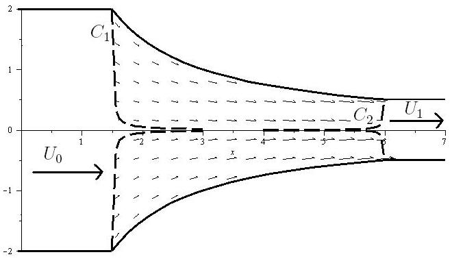
Figure 1: Extrusion die corresponding to the solution (142).

where the mean pressure $\sigma$ is given by (122), where we substitute the values of functions $u,v,\theta$ given by (145). The complex functions $c_{i}(t)$, $i=1,2,3$, and the real function $\sigma_{0}(t)$ which appear in this solution are arbitrary. For any time $t_{0}$, the solution (122), (145) has a singularity at point $(x_{0},y_{0})$ which satisfies the equation

$$x_{0}^{2}+y_{0}^{2}+2\left(\mathcal{R}e(c_{2}(t_{0}))x_{0}+\mathcal{I}m(c_{2}(t_{0}))y_{0}\right)+|c_{2}(t_{0})|^{2}=0.$$

This singularity is stationary if the function $c_{2}(t)$ is constant. Otherwise, its position varies with time. If the functions $\sigma_{0}$ and $c_{i}$, $i=1,2,3$, are of the form (142) defined in a region of the $xy$-plane on a time interval $[T_{0},T)$ where the gradient catastrophe does not occur, then the solution is bounded and damped. In figure 2, we have drawn the shape of an extrusion die corresponding to the solution (145) for the following choice of parameters: $\mathcal{R}e\left(c_{1}(t)\right)=0$, $\mathcal{I}m\left(c_{1}(t)\right)=0$, $\mathcal{R}e\left(c_{2}(t)\right)=0$, $\mathcal{I}m\left(c_{2}(t)\right)=-0.5$, $\mathcal{R}e\left(c_{3}(t)\right)=-0.5$ and $\mathcal{I}m\left(c_{3}(t)\right)=0$. The feeding velocity has component $U_{0}=0.2$, $V_{0}=0.2$, and the extraction of material is performed at the velocity $U_{1}=0.2$, $V_{1}=-0.2$. This type of tool can be used to bend a rod by extrusion without having to fold it. Finally, we should emphasize that the flow changes considerably when the parameters are varied and we have the freedom to choose the walls of the tool among the flow lines for certain fixed parameters $c_{i}(t)$. Moreover, the velocity and the orientation of the feeding (extraction) can vary somewhat for a given shape of the tool. Consequently, many types of extrusion dies can be drawn.

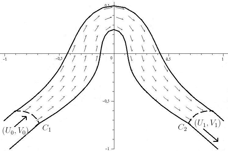
Figure 2: Extrusion die corresponding to the solution (145).

VII Final remarks

The generalized method of characteristics was originally devised for solving first-order quasilinear hyperbolic systems. The proposed techniques described in Sections III, IV and V allow us to extend the applicability of this approach not only to hyperbolic systems but also to encompass elliptic and mixed (parabolic) type systems, both homogeneous and inhomogeneous. A variant of the conditional symmetry method for obtaining multimode solutions has been proposed for these types of systems. We have demonstrated the usefulness of this approach through the examples of the nonlinear interaction of waves and particles and of the ideal plasticity in $(2+1)$ dimensions in its elliptic region. New classes of real solutions have been constructed in closed form, some of them bounded. Some of the obtained solutions describe a stationary flow for an appropriate choice of parameters. For these solutions, we have drawn extrusion dies and the vector fields which define the flow inside a region where the gradient catastrophe does not occur.

The proposed approach for constructing multimode solutions can be used in several potential applications arising from systems describing nonlinear phenomena in physics. It should be noted that in the multidimensional case, for many physical models, there are few known examples of multimode solutions written in terms of Riemann invariants for elliptic systems. This is a motivating factor for the elaboration of the generalization of the methods presented in Sections IV and V through the introduction of rotation matrices in the factorization of the Jacobian matrices (80). This fact weakens the integrability condition required in the expression (87). The approach proposed in this paper offers a new and promising way to construct and investigate such types of solutions. This makes our approach attractive since it can widen the potential range of applications leading to more diverse types of solutions.

Appendix: Derivation of the Jacobi Matrix (22)

In the appendix we present some details of the derivation of the equations (22). We use the notation introduced in the main text. Denote the $q\times q$ matrix

$$\psi=I_{q}-\left(\left(\frac{\partial f}{\partial r}+\frac{\partial\bar{f}}{\partial r}\right)\frac{\partial r}{\partial u}+\text{c.c.}\right)$$ (A.1)

Consequently, the expression for the Jacobian matrix (21) becomes

$$\psi^{-1}\left(\left(\frac{\partial f}{\partial r}+\frac{\partial\bar{f}}{\partial r}\right)\lambda+\text{c.c.}\right).$$ (A.2)

The expression (A.1) can also be written as

$$\psi=I_{q}-FS,$$ (A.3)

where the matrices $F$ and $S$ are defined in terms of the block matrices ${\partial f}/{\partial r}+{\partial\bar{f}}/{\partial r}\in\mathbb{R}^{q\times k}$ and ${\partial r}/{\partial u}\in\mathbb{R}^{k\times q}$ together with their complex conjugates

$$\begin{gathered}F=\left(\frac{\partial f}{\partial r}+\frac{\partial\bar{f}}{\partial r},\frac{\partial f}{\partial\bar{r}}+\frac{\partial\bar{f}}{\partial\bar{r}}\right)\in\mathbb{R}^{q\times 2k},\\ S=\left(\begin{array}[]{c}\frac{\partial r}{\partial u}\\ \frac{\partial\bar{r}}{\partial u}\\ \end{array}\right)\in\mathbb{R}^{2k\times q}.\end{gathered}$$ (A.4)

We multiply equation (A.3) on the right by the matrix $F$ in order to obtain

$$\psi F=F-FSF=F(I_{2k}-SF)=F\Phi,$$ (A.5)

where

$$\Phi=I_{2k}-SF.$$ (A.6)

Assuming that $\psi$ and $\Phi$ are invertible, the relation

$$\psi^{-1}F=F\Phi^{-1}$$ (A.7)

is satisfied. Using the notations (A.3) and (A.4), the Jacobian matrix (A.2) can be written in the compact form

$$\partial u=\psi^{-1}F\Lambda,\quad\Lambda=\left(\lambda,\bar{\lambda}\right)^{T}.$$ (A.8)

Replacing (A.7) into (A.8), we obtain the expression for the Jacobian matrix

$$\partial u=F\Phi^{-1}\Lambda.$$ (A.9)

We express the inverse of the matrix

$$\Phi=\left(\begin{array}[]{cc}\mathcal{A}&\mathcal{B}\\ \bar{\mathcal{B}}&\bar{\mathcal{A}}\end{array}\right)$$ (A.10)

in terms of the block matrices

$$\mathcal{A}=I_{k}-\frac{\partial r}{\partial u}\left(\frac{\partial f}{\partial r}+\frac{\partial\bar{f}}{\partial r}\right),\quad\mathcal{B}=\frac{\partial r}{\partial u}\left(\frac{\partial f}{\partial\bar{r}}+\frac{\partial\bar{f}}{\partial\bar{r}}\right),$$ (A.11)

where $\bar{\mathcal{A}}$ and $\bar{\mathcal{B}}$ are the complex conjugates of $\mathcal{A}$ and $\mathcal{B}$ respectively. Assuming that the block $\mathcal{A}$ is invertible, the matrix $\Phi$ is also invertible when

$$\det\Phi=\det\left(\mathcal{A}\right)\left(\bar{\mathcal{A}}-\bar{\mathcal{B}}\mathcal{A}^{-1}\mathcal{B}\right)\neq 0.$$

Consequently, we require that

$$\det\mathcal{A}\neq 0,\qquad\bar{\mathcal{A}}-\bar{\mathcal{B}}\mathcal{A}^{-1}\mathcal{B}\neq 0.$$ (A.12)

It should be noted that for $r$ and $f(r,\bar{r})$ of class $C^{2}$, the matrix $\mathcal{A}$ is the identity $I_{k}$ in the neighborhood of $x=0$, and it has to be invertible. Under the assumption (A.12), the inverse of the matrix $\Phi$ is given by

$$\Phi^{-1}=\left(\begin{array}[]{cc}M^{1}&M^{2}\\ \bar{M}^{1}&\bar{M}^{2}\end{array}\right),$$ (A.13)

where

$$M^{1}=\left(\mathcal{A}-\mathcal{B}\bar{\mathcal{A}}^{-1}\bar{\mathcal{B}}\right)^{-1},\quad M^{2}=-M^{1}\mathcal{B}\bar{\mathcal{A}}^{-1}.$$ (A.14)

Indeed,

$$\left(\begin{array}[]{cc}M^{1}&M^{2}\\ \bar{M}^{1}&\bar{M}^{2}\end{array}\right)= \left(\begin{array}[]{cc}M^{1}\mathcal{A}+M^{2}\mathcal{B}&\quad M^{1}\mathcal{B}+M^{2}\bar{\mathcal{A}}\\ \bar{M}^{2}\mathcal{A}+\bar{M^{2}}\mathcal{B}&\quad\bar{M}^{2}\mathcal{B}+\bar{M}^{1}\bar{\mathcal{A}}\end{array}\right)$$ (A.15)

$$= \left(\begin{array}[]{cc}M^{1}(\mathcal{A}-\mathcal{B}\bar{\mathcal{A}}^{-1}\bar{\mathcal{B}})&M^{1}(\mathcal{B}-\mathcal{B}\bar{\mathcal{A}}^{-1}\bar{\mathcal{A}})\\ \bar{M}^{1}(-\bar{\mathcal{B}}\mathcal{A}^{-1}\mathcal{A}+\bar{\mathcal{B}})&\bar{M}^{1}(-\mathcal{B}\mathcal{A}^{-1}\mathcal{B}+\bar{\mathcal{A}})\end{array}\right)$$

$$= \left(\begin{array}[]{cc}I_{k}&0\\ 0&I_{k}\end{array}\right)=I_{2k}.$$

Replacing the expression (A.13) for the matrix $\Phi^{-1}$ into equation (A.9), we obtain the form (22) for the Jacobian matrix. Next, substituting the equations (A.11) into the conditions (A.12) and into the matrices (A.14), we find the inequalities (LABEL:eq:3.11) and the equations (23), respectively.

References

- [1] M.J. Ablowitz, P.A. Clarkson, Solitons, Nonlinear evolution equations and inverse scattering, London Math. Soc. Lecture note ser 149, Cambrige Univ. Press. (1992).
- [2] G. Boillat, Sur la propagation des ondes., Gauthier-Villars, Paris, (1965).
- [3] M. Burnat, The method of Riemann invariants and its applications to the theory of plasticity, Com. Arch. Mech. Stos., part 1, 26, 6, 1974, 817-838 and part 2, 24, 1, 3-26 (1972).
- [4] E. Cartan, Sur la structure des groupes infinis de transformations, Chapt. 1: Les systèmes différentielles en involution, Gauthier-Villars, Paris, (1953).
- [5] J. Chakrabarty, Theory of Plasticity, Elsevier, (2006).
- [6] R. Conte, A.M. Grundland, B. Huard, Elliptic solutions of isentropic ideal compressible fluid flow in dimensions, J. Phys. A: Math. Theor. 42, 135203, 14pp, (2009).
- [7] R. Courant, D. Hilbert, Methods of mathematical physics. vol 1 and 2, Interscience, New-York, (1962).
- [8] J. Czyz, Construction of a flow of an ideal plastic material in a die, on the basis of the method of Riemann invariants, Archives of Mechanics, 26(4), 589-616, (1974).
- [9] P.W. Doyle, A.M. Grundland, Simple waves and invariant solutions of quasiliear systems, J. Math. Phys.,37, 6, 2969-2979, (1996).
- [10] B.A. Dubrovin and S.P. Novikov, Hamiltonnian formalism of one-dimensional systems of hydrodynamic type, Sov. Math. Dokl., 27, 665-669,(1983).
- [11] E.V. Ferapontov, K.R. Khusnutdinova, On the integrability of dimensional quasilinear systems, Com. Math. Phys.,248, 187-206, (2004).
- [12] E.V. Ferapontov, K.R. Khusnutdinova, The characterization of two-component (2+1)-dimensional integrable systems of hydrodynamic type, J. Phys. A: Math. Gen.,37, 2949-2963,(2004).
- [13] W. Fushchych, Conditional symmetry of equations of mathematical Physics, Ukrain Math. J.,43, 1456-1470, (1991).
- [14] A.M. Grundland, B. Huard, Riemann invariants and rank- solutions of hyperbolic systems, J. Nonlin. Math. Phys., 13,3, 393-419, (2006).
- [15] A.M. Grundland, B. Huard, Conditional symmetries and Riemann invariants for hyperbolic systems of PDEs, J. Phys. A, Math. Theor. 40, 4093-4123, (2007).
- [16] A.M. Grundland, J. Tafel, Symmetry reduction and Riemann wave solutions, J. Math. Anal. Appl.,198, 879-892, (1996).
- [17] A.M. Grundland, P. Vassiliou, On the solvability of the Cauchy problem for the Riemann double waves by the Monge-Darboux method. Analysis 11, 221-278, (1991).
- [18] A.M. Grundland, R. Zelazny, Simple waves in quasilinear systems, Part I and Part II, J. Math. Phys., 24, 9, 2305-2329, (1983).
- [19] A.M.Grundland, Riemann invariants for nonhomgeneous systems of quasilinear partial differential equations, Com. Bull. Acad. Polon. Sci., Ser Sci Techn 22, 273-282, (1974).
- [20] R. Hill, The Mathematical Theory of plasticity, Oxford University press, (1998).
- [21] E.L. Ince, Ordinary differential equations, Dover Publ. New-York, (1956).
- [22] A. Jeffrey, Quasilinear hyperbolic systems and wave propagation, Pitman Publ., (1976).
- [23] F. John, S. Klainerman, Almost global existence of nonlinear wave equations in three space dimensions, Com. Pure and Appl. Math., 37, 443-455, (1984).
- [24] E. Kamke, Differentialgleichungen, Lösungsmethoden und Löseungen, I B.G. Teubner Stuttgart, (1983).
- [25] L. Katchanov, Éléments de la théorie de la plasticité, Éditions Mir, Moscou, (1975).
- [26] M. Kuranishi, Lectures on involutive systems of partial differential equations. Publ. Brasil Math. Soc., Sao Paulo, (1967).
- [27] V. Lamothe, Symmetry group analysis of an ideal plastic flow. J. Math. Phys., 53, 3, 033704, (2012).
- [28] V. Lamothe, Group analysis of an ideal plasticity model, J. Phys. A: Math. Theor., 45, 285203, (2012).
- [29] R. K. Luneburg, Mathematical theory of optics, University of California Press, (1964).
- [30] R. Mises, Mathematical theory of compressible fluid flow, Acad. Press, New-York, (1958).
- [31] P.J. Olver, Applications of Lie Groups to Differential Equations, Springer-Verlag, New-York, (1986).
- [32] P.J. Olver, E. Vorobev, Nonclassical and conditional symmetries, Hankbook of Lie group analysis, Ed. N. Ibragimov, vol.3 chapt., 11 CRC Press, London, (1995).
- [33] Z. Peradzynski, Geometry of interactions of Riemann waves, Avances in nonliear waves vol. 2, Ed. Debnath, Research Notes in Mathematics no 111, Pitman Avanced Publ. Boston, (1985).
- [34] B.L. Rozdestvenski, N.N. Janenko, Systems of Quasilinear Equations and their Applications to Gas Dynamics, Transl. Math. Monographs, vol. 55, AMS Providence (1983).
- [35] S. Sobolev, Functionally invariant solutions of wave equations, Trudy phys. math. Inst. Steklova (in Russian),5, 259-264, (1934).
- [36] G.B. Whitham, Linear and nonlinear waves, John-willey Publ, New-York, (1974).
- [37] V.E. Zakharov, Nonlinear waves weak turbulence, in serie Advances of Modern Mathematics, (1998).