A spectral line survey of the starless and proto-stellar cores detected by BLAST toward the Vela-D molecular cloud

Abstract

Context. Starless cores represent a very early stage of the star formation process, before collapse results in the formation of a central protostar or a multiple system of protostars.

Aims. We use spectral line observations of a sample of cold dust cores, previously detected with the BLAST telescope in the Vela-D molecular cloud, to perform a more accurate physical and kinematical analysis of the sources.

Methods. We present a 3-mm and 1.3-cm survey conducted with the Mopra 22-m and Parkes 64-m radio telescopes of a sample of 40 cold dust cores, including both starless and proto-stellar sources. 20 objects were also mapped using molecular tracers of dense gas. To trace the dense gas we used the molecular species NH₃, N₂H⁺, HNC, HCO⁺, H¹³CO⁺, HCN and H¹³CN, where some of them trace the more quiescent gas, while others are sensitive to more dynamical processes.

Results. The selected cores have a wide variety of morphological types and also show physical and chemical variations, which may be associated to different evolutionary phases. We find evidence of systematic motions in both starless and proto-stellar cores and we detect line wings in many of the proto-stellar cores. Our observations probe linear distances in the sources $\ga 0.1\,$pc, and are thus sensitive mainly to molecular gas in the envelope of the cores. In this region we do find that, for example, the radial profile of the N₂H${}^{+}(1-0)$ emission falls off more quickly than that of C-bearing molecules such as HNC$(1-0)$, HCO${}^{+}(1-0)$ and HCN$(1-0)$. We also analyze the correlation between several physical and chemical parameters and the dynamics of the cores.

Conclusions. Depending on the assumptions made to estimate the virial mass, we find that many starless cores have masses below the self-gravitating threshold, whereas most of the proto-stellar cores have masses which are near or above the self-gravitating critical value. An analysis of the median properties of the starless and proto-stellar cores suggests that the transition from the pre- to the proto-stellar phase is relatively fast, leaving the core envelopes with almost unchanged physical parameters.

1 Introduction

Starless cores represent a very early stage of the star formation process, before collapse results in the formation of a central protostar or a multiple system of protostars. The physical properties of these cores can reveal important clues about their nature. Mass, spatial distributions, and lifetime are important diagnostics of the main physical processes leading to the formation of the cores from the parent molecular cloud.

In the past, (sub)millimeter continuum surveys performed with ground-based instruments have probed the Rayleigh-Jeans tail of the spectral energy distribution (SED) of these cold objects, far from its peak and, at short submillimeter wavelengths, have been affected by low sensitivity due to atmospheric conditions. Therefore, these surveys have been limited by their sensitivity or by their relative inadequacy to measure the temperature (e.g., Motte et al. 1998), producing large uncertainties in the derived luminosities and masses. Recent surveys with the MIPS instrument of the Spitzer Space Telescope are able to constrain the temperatures of warmer objects (Carey et al. 2005), but the youngest and coldest objects are potentially not detected, even in the long-wavelength Spitzer bands.

On the other hand, the more recent surveys with both the BLAST (“Balloon-borne Large-Aperture Submillimeter Telescope”, Pascale et al. 2008) and Herschel telescopes (see, e.g., Netterfield et al. 2009, Olmi et al. 2009, Molinari et al. 2010) have demonstrated the ability to detect and characterize cold dust emission from both starless and proto-stellar sources, constraining the low temperatures of these objects ($T\la 25$ K) using their multi-band photometry near the peak of the cold core SED. The bolometric observations alone, however, cannot fully contrain the dynamical and evolutionary status of the cores. Spectral lines follow-ups are necessary in order to investigate the physical, dynamical and chemical status of each detected core.

BLAST has identified more than a thousand new starless and proto-stellar cores during its second long duration balloon science flight in 2006. BLAST detected these cold cores in a $\sim 50\,$deg² map of the Vela Molecular Ridge (VMR) (Netterfield et al. 2009). The VMR (Murphy & May 1991, Liseau et al. 1992) is a giant molecular cloud complex within the galactic plane, in the area $260\degr\la l\la 272\degr$ and $-2\degr\la b\la 3\degr$, hence located outside the solar circle. Its main properties have been recently revisited by Netterfield et al. (2009) and Olmi et al. (2009).

In particular, Olmi et al. (2009) used both BLAST and archival data to determine the SEDs and the physical parameters of each source detected by BLAST in the smaller region of Vela-D (see Figure 1), where observations from IR (Giannini et al. 2007) to millimeter wavelengths (Massi et al. 2007) were already available. Olmi et al. (2010) then used the spectral line data of Elia et al. (2007) to perform a first analysis of the dynamical state of the cores toward Vela-D. They found that $\sim 30-50$% of the BLAST cores are gravitationally bound, and that a significant number of cores would need an additional source of external confinement.

In this work we will use spectral line observations, both single-points and maps, of a sample of BLAST sources from Vela-D to perform a more accurate physical and kinematical analysis of the starless and proto-stellar cores. This paper is thus organized as follows: in Section 2 we describe the selected targets and molecular lines. In Section 3 we present the results of the analysis of the observed molecular line spectra and maps, describing the derived physical and kinematical parameters. We then further discuss these results in Section 4 and conclude in Section 5.

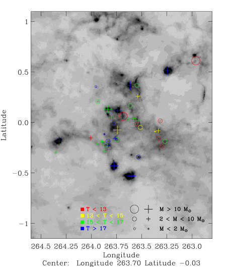
Figure 1: The gray-scale image shows the BLAST 250 $\mu$m map of Vela-D, with galactic coordinates in degrees. Superimposed are the locations of both starless (open circles) and proto-stellar (crosses) cores (see Olmi et al. 2009). The size of the symbols indicates the mass range [M_⊙] of each core and color-coding indicates the core temperature [K] (see legend).

Table 1: BLAST sources in Vela-D observed with the Mopra and Parkes telescopes

BLAST						Mopra		Parkes
Source #	Source name	$l$	$b$	Starless		Observation		Observation
		[deg]	[deg]	or Proto-Stellar		type		type
3	BLAST J084531-435006	263.6001	$-0.5302$	P		SP		SP
9	BLAST J084546-432458	263.3005	$-0.2341$	S		SP & M		SP
12	BLAST J084552-432152	263.2707	$-0.1886$	S		SP		–
13	BLAST J084606-433956	263.5331	$-0.3425$	S		M		–
14	BLAST J084612-432337	263.3322	$-0.1585$	S		SP & M		SP
23	BLAST J084633-432100	263.3370	$-0.0827$	P		SP		–
24	BLAST J084633-435432	263.7742	$-0.4309$	P		SP & M		SP
26	BLAST J084637-432245	263.3685	$-0.0899$	P		SP		–
31	BLAST J084654-431626	263.3177	$0.0149$	S		SP & M		SP
34	BLAST J084718-432804	263.5147	$-0.0496$	S		SP & M		SP
38	BLAST J084731-435344	263.8713	$-0.2886$	P		SP		SP
40	BLAST J084735-432829	263.5521	$-0.0141$	S		SP & M		SP
41	BLAST J084736-434332	263.7488	$-0.1699$	S		SP & M		SP
43	BLAST J084738-434931	263.8305	$-0.2277$	P		SP		SP
44	BLAST J084739-432623	263.5322	$0.0167$	P		SP		–
45	BLAST J084742-434347	263.7637	$-0.1582$	P		SP		SP
47	BLAST J084744-435045	263.8591	$-0.2249$	S		SP & M		SP
50	BLAST J084749-434810	263.8349	$-0.1861$	S		SP & M		SP
52	BLAST J084754-432748	263.5802	$0.0387$	P		SP		–
53	BLAST J084759-433942	263.7428	$-0.0757$	P		SP		–
54	BLAST J084801-435108	263.8947	$-0.1907$	P		SP		–
55	BLAST J084803-433051	263.6369	$0.0281$	S		M		–
56	BLAST J084805-435415	263.9430	$-0.2138$	S		SP & M		–
57	BLAST J084813-423730	262.9644	$0.6103$	S		SP & M		SP
59	BLAST J084815-434714	263.8713	$-0.1166$	P		SP		SP
63	BLAST J084822-433152	263.6856	$0.0609$	S		SP & M		SP & M
65	BLAST J084823-433858	263.7799	$-0.0106$	S		SP		–
71	BLAST J084834-435455	264.0059	$-0.1538$	P		SP		–
72	BLAST J084834-432430	263.6126	$0.1657$	S		SP		–
77	BLAST J084842-431735	263.5392	$0.2584$	P		SP		SP
79	BLAST J084844-433733	263.8007	$0.0525$	P		SP		–
81	BLAST J084847-425423	263.2482	$0.5133$	P		SP & M		SP
82	BLAST J084848-433225	263.7415	$0.1155$	P		SP & M		SP
88	BLAST J084910-441636	264.3543	$-0.2984$	P		SP		–
89	BLAST J084912-431353	263.5480	$0.3668$	S		SP & M		SP
90	BLAST J084912-433618	263.8379	$0.1312$	P		SP		SP
93	BLAST J084925-431710	263.6165	$0.3645$	P		SP		SP
97	BLAST J084932-441046	264.3206	$-0.1857$	P		SP		SP
101	BLAST J084952-433808	263.9381	$0.2058$	S		M		–
109	BLAST J085033-433318	263.9551	$0.3532$	S		M		–

Table 2: Molecular species observed with the Parkes and Mopra telescopes

Spectral line	$E_{\rm u}$	$n_{\rm eff}$	Rest Frequency
	[K]	[$\times 10^{3}\,$cm-3]	[MHz]
NH${}_{3}(1,1)$	23.4	$-$	23694.496
NH${}_{3}(2,2)$	64.9	$-$	23722.633
N2H${}^{+}(1_{21}-0_{32})$	4.47	2.5	93172.053
HNC$(1_{2}-0_{1})$	4.35	9.5	90663.574
HCO${}^{+}(1-0)$	4.28	2.5	89188.526
H13CO${}^{+}(1-0)$	4.16	2.2	86754.330
HCN$(1_{2}-0_{1})$	4.25	28	88631.847
H13CN$(1_{2}-0_{1})$	4.14	20	86340.167

2 Observations and archival data

2.1 Targets and lines selection

The observations were performed in June 2009 with the Mopra and Parkes telescopes of the Australia Telescope National Facility (ATNF). Although originally our aim was to observe all sources in the catalog of Olmi et al. (2009), because of time constraints we were able to observe a total of 40 sources at Mopra and 22 sources at Parkes, in either mapping or single-pointing mode (or both, see Table 1 and Figure 1). We have selected an almost equal number of starless (19) and proto-stellar (21) cores where, following Olmi et al. (2009), we define the BLAST cores as proto-stellar when they turned out to be positionally associated with one or more MIPS sources at 24$\,\mu$m, and starless otherwise. Each sub-sample is composed by objects that present increasing temperature and different morphology. This selection criterion is quite arbitrary but aimed at identifying different evolutionary stages within each sub-sample.

In order to probe the dense and cold gas detected by BLAST toward the cores in Vela-D we needed appropriate molecular tracers. We thus selected several rotational transitions with low quantum numbers to be observed at Mopra in the 3-mm band, and we also observed the NH₃(1,1) and (2,2) inversion lines with the Parkes telescope. In the following sections, our analysis will be based on the ammonia lines and on the main spectral lines observed at Mopra, i.e., N₂H${}^{+}(1-0)$, HCN$(1-0)$, HNC$(1-0)$ and HCO${}^{+}(1-0)$ (and two of their isotopologues, see Table 2). This choice of molecular tracers ensured that we would be able to trace the dense as well as the more diffuse gas, and we would also be able to detect molecular outflows. Furthermore, these molecules should also be able to give out clues about the different chemical states of the sources.

2.2 Mopra

During the spectral line mapping or single-pointing mode observations with the Mopra telescope the system temperatures were typically comprised in the range $\sim 170-280\,$K and we reached a RMS sensitivity in $T_{\rm A}^{\star}$ units of about $\sim 30-40\,$ mK after rebinning to a 0.22 km s^-1 velocity resolution. The beam full width at half maximum (FWHM) was about $38\,$arcsec and the pointing was checked every hour by using an SiO maser as a reference source. Typically, pointing errors were found to be $\sim 5-10\,$arcsec.

The parameter $\eta_{\rm mb}$ to convert from antenna temperature to main-beam brightness temperature has been assumed to be 0.44 at 100 GHz and 0.49 at 86 GHz (Ladd et al. 2005). The Mopra spectrometer (MOPS) was used as a backend instrument in its “zoom” mode, which allowed to split the 8.3 GHz instantaneous band in up to 16 zoom bands; each sub-band was 137.5 MHz wide and had 2$\times$4096 channels. The single-point observations were performed in position-switching mode, whereas the spectral line maps, of size mostly $3\times 3\,$arcmin², were obtained using the Mopra on-the-fly mapping mode, scanning in both right ascension and declination.

The most intense lines observed were N₂H${}^{+}(1-0)$, HCN$(1-0)$, HNC$(1-0)$ and HCO${}^{+}(1-0)$. These lines are all good tracers of dense gas, and are also often used to detect velocity gradients. N₂H⁺ is known to be more resistant to freeze-out on grains than the carbon-bearing species. HNC is particularly prevalent in cold gas (Hirota et al. 1998), while HCO⁺ often shows infall signatures and outflow wings. These strong lines can all be optically thick and thus two isotopologues, H¹³CO⁺ and H¹³CN, were also observed to provide optical depth and line profile information. Unfortunately, their intensity was in general too weak to allow derivation of column densities throughout the maps and other useful physical and kinematical parameters, and thus most of our analysis will be based on the four most intense molecular tracers.

2.3 Parkes

A total of 22 sources where observed with the Parkes telescope in single-pointing mode (see Table 1), and only one source (BLAST063) was mapped using the NH₃(1,1) and (2,2) transitions. The system temperatures were typically $\sim 40-50\,$K and we reached a RMS sensitivity in $T_{\rm A}^{\star}$ units of $\sim 10\,$mK after rebinning to a $\simeq 0.2\,$km s^-1 velocity resolution. The beam FWHM was about $1.3\,$arcmin and the pointing errors were found to be $<20\,$arcsec. The Parkes Multibeam correlator, in single-beam high resolution mode, was used as a backend. A simultaneous band of 64 MHz was observed, with a total of 8192 channels, which allowed to observe the NH₃(1,1) and (2,2) lines within the same bandwidth.

2.4 BLAST

BLAST is a 1.8 m Cassegrain telescope, whose under-illuminated primary mirror has produced in-flight beams with FWHM of 36 ″, 42 ″, and 60 ″ at 250, 350, and 500 $\mu$m, respectively. More details on the instrument, calibration methods and map-making procedure can be found in the BLAST05 papers Pascale et al. (2008), Patanchon et al. (2008), and Truch et al. (2008).

The Vela-D region, shown in Figure 1 and defined by Olmi et al. (2009) as the area contained within $262\aas@@fstack{\circ}80<l<264\aas@@fstack{\circ}60$ and $-1\aas@@fstack{\circ}15<b<1\aas@@fstack{\circ}10$, was part of a larger map of the Galactic Plane obtained by BLAST toward the VMR (Netterfield et al. 2009). In Vela-D Olmi et al. (2009) found a total of 141 sources, both starless and proto-stellar, and in the next sections we will follow the source numbering (0 to 140) defined by these authors.

Table 3: Peak intensity of main detected lines or the rms Level of the spectrum.

Source #	N2H+	HCN	H13CN	HNC	HC3N	HCO+	H13CO+
3	0.17	0.81	$<$0.03	0.58	–	0.70	0.13
9	0.09	0.06	$<$0.03	0.20	–	0.22	0.06
12	$<$0.02	0.05	$<$0.02	$<$0.03	–	0.07	$<$0.02
23	$<$0.02	0.10	$<$0.03	0.25	–	0.38	$<$0.03
24	1.33	2.97	0.23	2.23	–	3.20	0.32
26	$<$0.02	0.07	$<$0.02	0.08	–	0.14	$<$0.02
26	–	–	–	0.10	–	0.13	–
31	$<$0.02	0.11	$<$0.02	0.15	–	0.34	$<$0.02
34	$<$0.02	0.08	$<$0.02	0.07	–	0.23	$<$0.02
34	–	–	–	–	–	0.15	–
38	0.07	0.11	$<$0.02	0.15	–	0.19	$<$0.02
40	0.20	0.31	$<$0.02	0.45	–	0.73	0.28
41	$<$0.02	0.27	$<$0.03	0.20	–	0.41	$<$0.02
43	$<$0.05	0.11	$<$0.05	0.26	–	0.42	$<$0.05
44	0.21	0.35	$<$0.04	0.57	–	0.88	0.13
45	0.13	0.24	$<$0.02	0.24	–	0.52	$<$0.02
47	$<$0.02	0.19	$<$0.02	0.12	–	0.14	$<$0.02
47	–	–	–	–	–	0.13	–
50	$<$0.02	0.10	$<$0.02	0.07	–	0.16	$<$0.02
52	$<$0.02	0.11	$<$0.02	0.10	–	0.18	$<$0.02
53	0.07	0.20	$<$0.02	0.28	–	0.19	0.07
54	$<$0.02	0.14	$<$0.02	0.12	–	0.12	$<$0.02
56	$<$0.02	0.14	$<$0.03	0.08	–	0.16	$<$0.02
57	0.12	0.13	$<$0.03	0.21	–	0.33	0.13
59	0.12	0.18	$<$0.03	0.22	–	0.23	0.08
63	0.11	0.44	$<$0.02	0.55	–	0.76	0.09
65	$<$0.02	0.12	$<$0.02	0.09	–	0.15	$<$0.02
71	$<$0.04	0.11	$<$0.04	$<$0.05	–	$<$0.08	$<$0.04
72	$<$0.02	0.15	$<$0.02	0.14	–	0.39	$<$0.02
72	–	–	–	–	–	0.19	–
77	0.06	0.26	$<$0.02	0.23	–	0.45	$<$0.03
79	$<$0.05	0.17	$<$0.05	0.23	–	0.22	$<$0.05
81	1.49	4.32	0.39	2.42	–	4.31	0.25
82	0.50	0.65	$<$0.03	0.74	–	1.30	0.23
88	$<$0.02	0.26	$<$0.03	0.18	–	$<$0.02	$<$0.03
89	$<$0.02	0.16	$<$0.02	0.09	–	0.22	$<$0.03
90	0.50	1.32	0.12	1.30	0.16	2.19	0.38
93	0.50	0.75	0.11	1.03	0.26	1.45	0.44
97	0.19	0.54	$<$0.03	0.62	–	0.79	0.12

3 Results

In this section we will discuss the derivation of various physical parameters such as column density, mass and kinetic temperature, that are fundamental for the analysis of the sources. We will also analyse the kinematics of the sources, determining velocity gradients and line asymmetries. The estimate of the virial masses will also allow us to determine which sources are currently gravitationally bound and which are not.

3.1 Morphological characteristics of spectral line maps

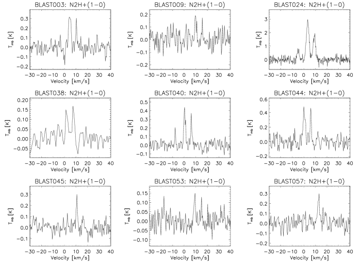
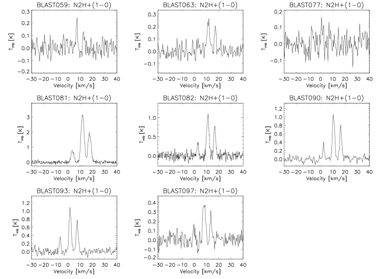
Figure 15: Spectra of N₂H${}^{+}(1-0)$ towards the Vela-D sources.

The spectral line data and maps were reduced and analyzed using the standard IRAM package CLASS, and the XS package of the Onsala Space Observatory. The single-point spectra obtained with the Mopra telescope towards the nominal position of the BLAST cores are shown in Figures 15 to 21 of the Appendix. The peak intensities of the detected lines, or the spectrum RMS in case of no detection, are listed in Table 3. Tables 12 to 15 in the Appendix list several physical and kinematical parameters of the sources.

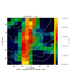
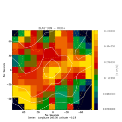
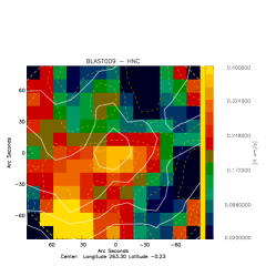
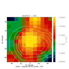
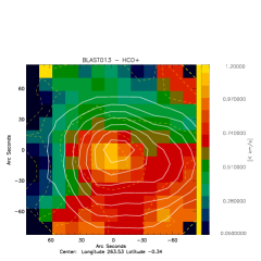
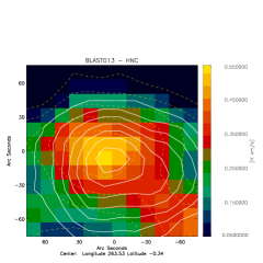
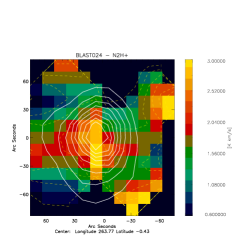
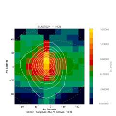
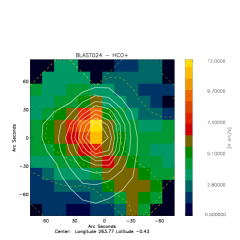
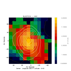
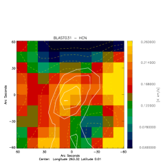
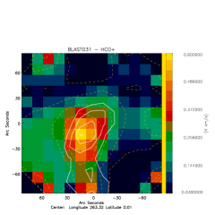
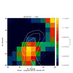
Figure 11: Maps of the line integrated intensities (from left to right, N₂H${}^{+}(1-0)$, HCN$(1-0)$, HCO${}^{+}(1-0)$ and HNC$(1-0)$, in units of $\int T_{\rm A}^{\star}\,{\rm d}v$ [K km s${}^{-1}]$) of selected sources toward Vela-D. In this figure we show, from top to bottom, maps of BLAST009, BLAST013, BLAST024 and BLAST031. The white dashed contours represent the BLAST flux density at 250 $\mu$m.

The multi-line integrated intensity maps obtained at Mopra, with the most significant SNR, are shown in Figure 11 to 14 of the Appendix, where the white contours represent the BLAST emission at 250$\,\mu$m. One can see that in general the line emission follows the dust continuum emission, even when the emission is more diffuse and filamentary as observed, for example, in source BLAST063. But we also note that in several sources (for example, BLAST055, BLAST056, BLAST081 and BLAST101) the dust continuum and some of the line emission peak at different positions.

One can immediately note that the three proto-stellar cores that were mapped (BLAST024, BLAST081 and BLAST082) have a much more regular shape than the starless ones. We also note that the maps of sources BLAST024 and BLAST081 are partly affected by artefacts, likely caused by bad weather during the observations at Mopra, which show up as sharp drops of the integrated intensity, particularly in the maps of the HCO${}^{+}(1-0)$ line. We can also see that in source BLAST082 two separate, smaller cores have been identified. In terms of the molecular tracers observed, we note that there are clear differences in the spatial distribution of emission from different molecular species. These morphological differences are more evident in the starless cores (but also, for example, in the proto-stellar core BLAST081) and suggest both physical and chemical differences among the observed sources.

We may summarize the wide variety of spatial morphologies observed as follows: very early and cold starless cores appear to have an irregular shape (e.g., BLAST009) in most or all molecular tracers mapped at Mopra. Some warmer cores (e.g., BLAST031) and cores at the transition phase from starless to proto-stellar (BLAST063, see Section 4.5) appear to be more compact. Finally, proto-stellar cores all show a more regular shape and narrow radial intensity profiles (see Section 3.6). Throughout the rest of the paper we will thus discuss how, besides to morphological differences, these cores also show physical and chemical variations, which may be associated to different evolutionary phases.

Table 4: NH₃(1,1) line parameters.

Source #	NH3(1,1)
	$T_{A}^{\star}\,\tau$	$V_{\rm lsr}$	$FWHM$	$\tau$
	[K]	[km s-1]	[km s-1]
3	0.15	5.3	1.9	1.40
9	0.04	10.7	1.1	0.66
14	0.13	3.0	0.7	2.63
24	0.38	3.5	2.6	0.51
31	0.06	10.7	1.3	2.77
40	0.07	1.3	0.9	0.22
41	0.05	11.1	0.7	0.10
47	0.04	5.5	1.5	0.77
57	0.07	14.0	1.5	1.73
63	0.11	12.4	1.7	0.94
77	0.05	2.0	0.8	0.10
81	0.06	12.3	3.1	0.10
82	0.11	11.7	2.0	0.22
90	0.10	11.4	1.7	0.10
93	0.13	2.4	1.2	0.70
97	0.31	9.4	1.6	1.28

Table 5: NH₃(2,2) line parameters.

Source #	NH3(2,2)
	$\int{T_{A}^{\star}\,{\rm d}V}$	$V_{lsr}$	FWHM
	[K km s-1]	[km s-1]	[km s-1]
3	0.06	5.3	1.1
24	0.54	3.6	3.1
47	0.03	5.3	2.9
63	0.03	10.3	1.8
81	0.08	12.2	2.7
82	0.07	11.7	1.9
90	0.06	11.4	2.5
93	0.07	2.4	1.8
97	0.14	9.3	2.1

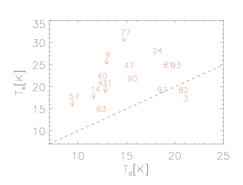
Figure 2: Kinetic temperature, $T_{\rm k}$, as derived from the NH₃(1,1) and (2,2) inversion transitions, vs. the BLAST-derived dust temperature, $T_{\rm d}$. Sources are identified through their ID (see Table 1), and the vertical arrows indicate that the corresponding $T_{\rm k}$ is an upper limit. The dashed line indicates the $T_{\rm k}=T_{\rm d}$ locus.

3.2 Temperature and optical depth from hyperfine structure fits

The excitation temperature, $T_{\rm ex}$, and the line optical depth, $\tau$, which are required to estimate the molecular column densities (see Sect. 3.5.1) could only be determined in those sources where molecules with a hyperfine structure (hfs, hereafter) were detected, i.e., N₂H⁺, HCN and H¹³CN, and/or when both the HCO${}^{+}(1-0)$ and H¹³CO${}^{+}(1-0)$ lines were detected.

In the molecules with a hfs, we used method “hfs” of the CLASS program to determine both $T_{\rm ex}$ and $\tau$. In those cases where both HCO⁺ and H¹³CO⁺ were detected, the optical depth was estimated from their line intensity ratio, assuming the same excitation temperature for the two isotopic molecular species and using the abundance ratio [HCO⁺]/[H¹³CO⁺]$\simeq 40$ (Zinchenko et al. 2009).

For the purpose of estimating the column density later, in those sources where the hfs method could not be used for one or more molecules (for example because of low SNR), or if only HCO⁺ was detected but not H¹³CO⁺, the values of both $T_{\rm ex}$ and $\tau$ for a given molecular species were assumed to be the averages of the parameters estimated from the detected molecular transitions in the same source.

3.3 Temperature and optical depth from NH₃

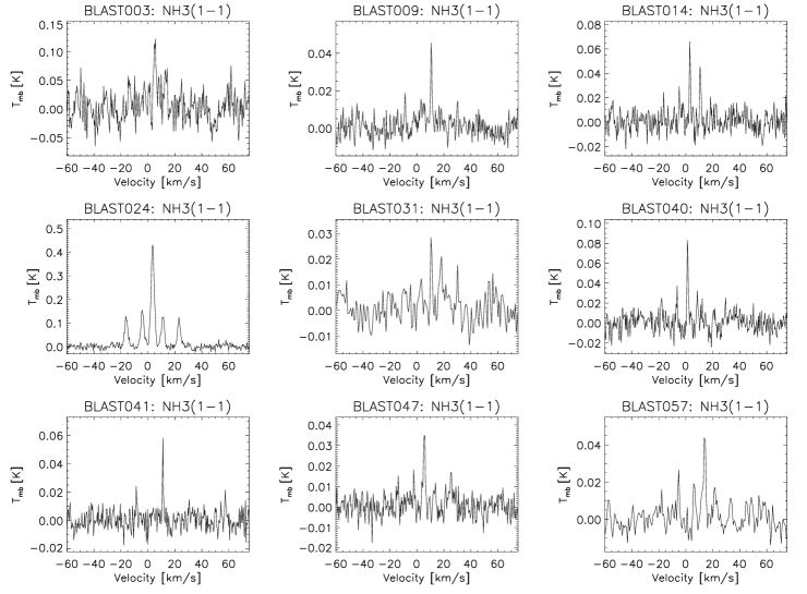
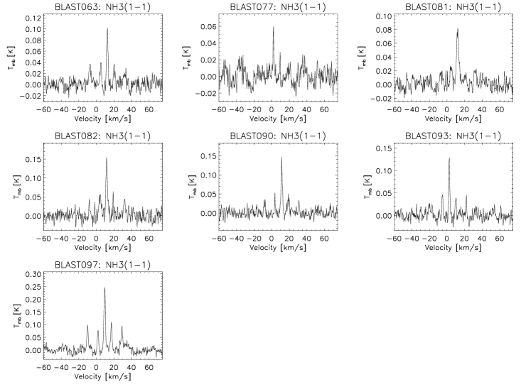
Figure 22: Spectra of the NH₃(1,1) line obtained with the Parkes telescope.

The single-point spectra of the NH₃(1,1) inversion line, obtained with the Parkes telescope, are shown in Figure 22 of the Appendix. The (2,2) line has been detected towards nine sources (mostly proto-stellar). We attempted to map the NH₃(1,1) transition toward BLAST063, but we did not detect the line due to insufficient SNR in the individual scanning positions.

Method “nh3” of the CLASS program, similar to method “hfs” described above, was used to fit the NH₃(1,1) line and resulted in the parameters $T_{A}^{\star}\,\tau$, $\tau$ and FWHM listed in Table 4. Due to the fact that the hfs components of the NH₃(2,2) line were not detected (with the exception of source BLAST024), the line parameters were derived from a standard Gaussian fit to the main component of the NH₃(2,2) hyperfine structure and are listed in Table 5.

Table 6: Results of velocity gradient fitting.

Source #	HNC$(1-0)$				HCO${}^{+}(1-0)$
	$V_{o}$	${\rm d}V/{\rm d}r$	$\theta_{v}$		$V_{o}$	${\rm d}V/{\rm d}r$	$\theta_{v}$
	[km s-1]	[km s-1 pc-1]	[deg]		[km s-1]	[km s-1 pc-1]	[deg]
9	$-$	$-$	$-$		12.2	0.8	88.5
13	1.0	2.3	21.1		0.9	1.5	18.1
24	5.5	1.9	60.7		5.3	1.7	57.7
34	$-$	$-$	$-$		2.6	1.6	224.1
40	2.5	0.2	16.7		2.6	1.2	71.5
41	$-$	$-$	$-$		12.1	1.2	289.9
47	6.6	2.7	240.1		$-$	$-$	$-$
63	13.0	1.6	55.2		13.2	1.3	86.8
81	13.5	1.4	256.9		13.3	1.9	312.6
82	13.6	2.1	15.7		13.0	1.5	334.5

We then determined the kinetic temperature, $T_{\rm k}$, and NH₃ column density using both NH₃(1,1) and (2,2) transitions, in those sources where the (2,2) line was indeed detected. In these cases we were able to determine the rotational temperature, $T_{\rm 12}$ (and thus $T_{\rm k}$), and the column density using the method of Ungerechts et al. (1986) and Bachiller et al. (1987). In this method the required data were: (i) the product $\tau(T_{\rm ex}-T_{\rm bg})$ for the (1,1) line, where $T_{\rm ex}$ and $T_{\rm bg}=2.725\,$K are the excitation and background temperatures, respectively, and $\tau$ is the optical depth; (ii) the linewidth $\Delta V(1,1)$; and (iii) the (2,2) integrated intensity. Once $T_{\rm 12}$ has been estimated, the kinetic temperature can be determined using the analytical expression of Tafalla et al. (2004):

$$T_{\rm k}=\frac{T_{\rm 12}}{1-\frac{T_{\rm 12}}{42}\ln[1+1.1\exp(-\frac{16}{T_{\rm 12}})]}$$ (1)

which is an empirical expression that fits the $T_{\rm 12}-T_{\rm k}$ relation obtained using a radiative transfer model. For those sources where the NH₃(2,2) transition was not detected, we could only determine an upper limit to $T_{\rm k}$ (shown in Figure 2). However, in order to obtain an estimate of the column density, and thus of the mass, for these sources we adopted the BLAST-derived temperature, $T_{\rm d}$, as an approximation for $T_{\rm k}$, which turns out to be a reasonably good assumption, as discussed below.

For those sources with an independent estimate of $T_{\rm k}$ we compared the resulting kinetic temperatures with the BLAST-derived dust temperatures, as obtained by Olmi et al. (2009), and we show the results in Figure 2. This comparison between $T_{\rm k}$ and $T_{\rm d}$, when applied separately to starless and proto-stellar cores, is affected by the few detections of NH₃(2,2) toward starless cores, and by the relatively high spread in the values of the $T_{\rm k}/T_{\rm d}$ ratio. In fact, for the two starless cores (BLAST047 and BLAST063; see also Section 4.5) where this ratio could be measured we obtain a mean value $\langle T_{\rm k}/T_{\rm d}\rangle=1.4$, whereas for the proto-stellar cores we get a median value $T_{\rm k}/T_{\rm d}=1.2\pm 0.2$.

When all cores are considered together, we get a median value $T_{\rm k}/T_{\rm d}=1.2\pm 0.2$, i.e., the median value is dominated by the proto-stellar cores. A tentative explanation for the fact that $T_{\rm k}$ tends to be slightly higher than $T_{\rm d}$ could be that the NH₃ observations are sampling regions that are somewhat warmer compared to the BLAST-derived $T_{\rm d}$ measurements. In fact, the BLAST observations are likely to average the temperature on much larger volumes of dust and, in addition, in the less dense regions there could be a systematic difference between $T_{\rm d}$ and $T_{\rm k}$. In the literature both cases of systematic departures between dust and gas temperature, i.e. $T_{\rm k}<T_{\rm d}$ or $T_{\rm k}>T_{\rm d}$, can be found (e.g., Kruegel & Walmsley 1984, Pirogov & Zinchenko 1993). The dust and gas temperature may be affected by various effects, and a more detailed analysis of these effects in our sources is beyond the scopes of the present work.

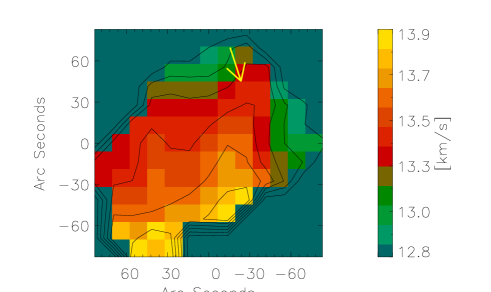
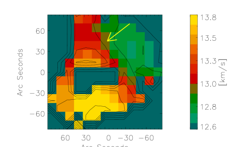
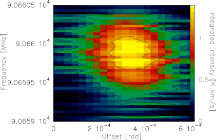
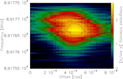
Figure 3: In the top panels we show the maps of the $V_{\rm lsr}$ for the HNC$(1-0)$ (left) and HCO${}^{+}(1-0)$ (right) lines toward the proto-stellar core BLAST081, as obtained from Gaussian fits to the spectra at each map position. The arrows show the direction of the velocity gradient, with their length proportional to the magnitudes listed in Table 6. The bottom panels show the position-velocity plots, with the horizontal axis representing the angular offset along a direction parallel to the velocity gradient shown by the arrows in the top panels. Note the different direction of the velocity gradient in the two molecular tracers.

3.4 Kinematics

3.4.1 Velocity gradients

We investigated the presence of systematic velocity gradients in those sources which could be mapped. In particular, the velocity gradient of a gas clump can be determined by using all or most of the data in a map at once, by least-squares fitting maps of line-center velocity for the direction and magnitude of the best-fit velocity gradient (see Goodman et al. 1993 and references therein).

A cloud undergoing solid-body rotation would exhibit a linear gradient, ${\rm d}V/{\rm d}r$, across the face of a map, perpendicular to the rotation axis. Thus, we have applied the procedure developed by Goodman et al. (1993) and Olmi & Testi (2002) to determine the magnitude and direction of the velocity gradient in our spectral line maps. Our best results are listed in Table 6, and are restricted to the HCO${}^{+}(1-0)$ and HNC$(1-0)$ lines. We note that for most sources with measured velocity gradients in both lines, the two separately estimated values of ${\rm d}V/{\rm d}r$ and $\theta_{v}$ are consistent, within a 50 % difference. However, the velocity gradient measured in the HNC map of core BLAST040 is quite small and thus its direction can be affected by large uncertainties. Thus the largest discrepancies between the two tracers are observed in the two proto-stellar cores BLAST081 and BLAST082, and also in the starless core BLAST013.

The position-velocity plots for the proto-stellar core BLAST081 are shown in Figure 3. The top panels show the maps of $V_{\rm lsr}$ for the HNC$(1-0)$ and HCO${}^{+}(1-0)$ lines, as obtained from Gaussian fits to the spectra at each observed position. The arrows represent the direction and magnitude of the velocity gradient as obtained from the procedure described above. We note the significant difference between the directions of the velocity gradients as measured in the HNC and HCO⁺ maps. It is not clear whether this discrepancy is real or may be caused by the presence of some artefacts in the HCO⁺ map of BLAST081, as noted in Section 3.1. On the other hand, source BLAST082 has no visible artefacts, and it is thus possible that in both proto-stellar cores the different velocity gradients in the HNC and HCO⁺ maps are real and are tracing different systematic motions. One of these velocity gradients could be associated with a molecular outflow, as suggested by the presence of line-wings in the HCO${}^{+}(1-0)$ spectra (see Table 15).

3.4.2 Line asymmetries

The HCO${}^{+}(1-0)$ line is generally the most intense transition observed with the Mopra telescope in each source, and it does not have a hyperfine structure. Therefore, it represents the ideal candidate to identify and analyze asymmetries of the line profile. In fact, the HCO${}^{+}(1-0)$ line shows a non-Gaussian profile toward several sources (see Table 15), and in some cases unambiguous wing emission is detected, indicating the likely presence of a molecular outflow. By inspecting Table 15 we also note a moderate shift, up to $\sim 1\,$km s^-1, between the peak positions of the generally optically thick HCO${}^{+}(1-0)$ line and optically thin H¹³CO${}^{+}(1-0)$ transition. We can give a quantitative estimate of this asymmetry in order to get some indirect information about dynamical processes in the cores.

A widely used method to extract line asymmetries is based on the comparison of optically thin and optically thick line velocities, i.e., determining the parameter $\delta V=(V_{\rm thick}-V_{\rm thin})/\Delta V_{\rm thin}$ (Mardones et al. 1997). In this way we can divide our cores in “blue shifted” cores, with $\delta V<0$, and “red shifted” cores with $\delta V>0$. The blue shifted values of $\delta V$ could be caused by infall motions and the red excess by expanding motions or outflow.

We identified 13 sources where the HCO${}^{+}(1-0)$ and H¹³CO${}^{+}(1-0)$ linewidths could be measured and in Figure 4 we show the distribution of their $\delta V$ parameter, with $V_{\rm thick}$ and $V_{\rm thin}$ being determined from the HCO${}^{+}(1-0)$ and H¹³CO${}^{+}(1-0)$ lines, respectively. We also estimated the typical error on $\delta V$ and then used the same $\pm 5\sigma_{\delta V}$ threshold as Mardones et al. (1997) to exclude those sources where the $V_{\rm lsr}$ differences were dominated by measurement errors. We estimated $5\sigma_{\delta V}\simeq 0.4-0.6$, thus in Figure 4 a typical value $5\sigma_{\delta V}\simeq 0.5$ is used. Only three cores show a significant blue shift (BLAST044, BLAST090 and BLAST093), and two a red shift (BLAST003 and BLAST053). From the red excess candidates we have to exclude BLAST053 which has a weak and noisy H¹³CO${}^{+}(1-0)$ spectrum.

Table 7: Mass estimates.

Source #			$M_{\rm cd}$
	$M_{\rm blast}$	$M_{\rm vir}$	N2H+	HNC	HCO+	HCN	NH3
	[$M_{\odot}$]	[$M_{\odot}$]	[$\times 10^{-9}M_{\odot}$]	[$\times 10^{-9}M_{\odot}$]	[$\times 10^{-9}M_{\odot}$]	[$\times 10^{-9}M_{\odot}$]	[$\times 10^{-7}M_{\odot}$]
3	23.2	68.1	$-$	$-$	$-$	$-$	$-$
9	3.1	15.9	$-$	2.6	1.6	0.3	7.9
13	6.4	$-$	$-$	3.7	7.6	3.5	$-$
14	7.7	8.9	$-$	$-$	$-$	$-$	$-$
24	98.0	87.3	5.4	25.7	54.1	17.8	5.8
31	4.0	26.4	$-$	0.02	2.3	0.6	31.8
34	4.6	$-$	$-$	2.1	1.9	$-$	$-$
38	2.2	32.4	$-$	$-$	$-$	$-$	$-$
40	6.3	11.3	0.13	4.9	13.9	2.5	2.1
41	2.8	10.8	$-$	$-$	7.4	$-$	0.8
44	5.8	19.1	$-$	$-$	$-$	$-$	$-$
45	2.1	17.6	$-$	$-$	$-$	$-$	$-$
47	2.6	44.7	$-$	2.2	2.7	5.7	4.6
50	2.3	$-$	$-$	$-$	6.0	9.9	$-$
53	11.6	25.9	$-$	$-$	$-$	$-$	$-$
56	1.8	$-$	$-$	0.1	1.5	0.6	$-$
57	14.0	27.0	$-$	$-$	8.7	$-$	$-$
59	1.8	17.5	$-$	$-$	$-$	$-$	$-$
63	13.4	64.6	1.5	4.7	10.3	8.3	9.0
77	3.7	12.3	$-$	$-$	$-$	$-$	$-$
81	69.9	88.8	2.2	13.4	40.4	14.2	0.6
82	16.5	42.2	2.4	8.1	29.8	4.2	1.4
89	2.4	$-$	$-$	$-$	6.7	$-$	$-$
90	22.2	43.9	$-$	$-$	$-$	$-$	$-$
93	15.2	17.7	$-$	$-$	$-$	$-$	$-$
97	24.4	54.5	$-$	$-$	$-$	$-$	$-$
101	2.1	$-$	$-$	1.0	3.5	0.9	$-$
109	1.0	$-$	$-$	$-$	0.9	$-$	$-$

3.5 Derivation of masses

From our spectral line data we can derive masses from the gas column density, $M_{\rm cd}$, as well as virial masses, $M_{\rm vir}$, which we can then compare with the BLAST-derived masses, $M_{\rm blast}$, estimated from the dust continuum. Clearly, while the virial masses refer to the total gas mass, with $M_{\rm cd}$ we can only determine the mass of a given molecular species. The total gas mass can only be determined by assuming specific molecular abundances; or, alternatively, we can give a coarse estimate of the molecular abundance by taking the ratio $M_{\rm cd}/M_{\rm blast}$ (see Section 4.1). The isotopologues observed by us, H¹³CO⁺ and H¹³CN, are generally too weak to allow derivation of column densities throughout the maps, and thus we use only the main molecular species, attempting to correct for first-order optical depth effects.

3.5.1 Mass derived from column density

The calculation of masses from the column density assumes LTE and we determine the molecular gas mass integrating the molecule column density over the extent of the source. Then we can write:

$$M_{\rm cd}=d^{2}\,m_{\rm mol}\,\int\,N_{\rm mol}\,{\rm d}\Omega$$ (2)

where $\int\,N_{\rm mol}\,{\rm d}\Omega$ is the molecule column density integrated over the region enclosed by the chosen contour level, $m_{\rm mol}$ is the mass of the specific molecule being considered, and $d$ is the distance to the source. The column density $N_{\rm mol}$ corresponding to a $J\rightarrow J-1$ rotation transition can be calculated as:

$$N_{\rm mol}\,[{\rm cm}^{-2}]=\frac{4.0\times 10^{12}}{J^{2}\mu^{2}[{\rm D}]\,B[{\rm K}]}Z\exp\left(\frac{E_{\rm J}}{T_{\rm ex}}\right)\times$$

$$\frac{1}{\eta_{\rm mb}}\frac{\tau}{1-e^{-\tau}}\int\,T_{\rm A}^{\star}\,{\rm d}v\,[{\rm K\leavevmode\nobreak\ km\leavevmode\nobreak\ s}^{-1}]$$ (3)

where $B$ denotes the rotational constant, $E_{\rm J}$ is the upper state energy, $\mu$ is the dipole moment (in Debye) and we used the escape probability $\tau/[1-\exp(-\tau)]$ to account for first-order optical depth effects. The derivation of both $T_{\rm ex}$ and $\tau$ has been discussed in Section 3.2. For $kT_{\rm ex}>>hB$ the partition function, $Z$, of a linear molecule is given by:

$$Z=\frac{kT_{\rm ex}}{hB}$$ (4)

where $h$ and $k$ are the Planck and Boltzmann constants, respectively.

Eq. (2) is actually implemented by writing:

$$M_{\rm cd}=d^{2}\,m_{\rm mol}\,\Delta\Omega_{\rm pix}\,\sum_{i=1}^{n_{\rm pix}}\,N_{\rm mol}(x_{i},y_{i})$$ (5)

where $N_{\rm mol}(x_{i},y_{i})$ represents the column density in a single pixel $(x_{i},y_{i})$ of the map, with $n_{\rm pix}$ representing the total number of pixels, and $\Delta\Omega_{\rm pix}$ represents the solid angle covered by a single pixel. The map pixels selected are those that have an integrated intensity $I\geq\sigma_{\rm map}$, and also lie within an $1/e$ radius from the center of a 2D Gaussian fit to the core, for each specific molecule. Assuming that a line is detected if at least two adjacent velocity channels lie above the $3\sigma_{\rm rms}$ level of the spectrum, then we calculate the RMS of the integrated intensity in the map simply as $\sigma_{\rm map}=2(3\sigma_{\rm rms})\Delta v$, where $\Delta v$ is the channel width. We thus select only those pixels that belong to the actual “core” of the source, and remove pixels that come from extended diffuse envelopes. The resulting masses are listed in Table 7.

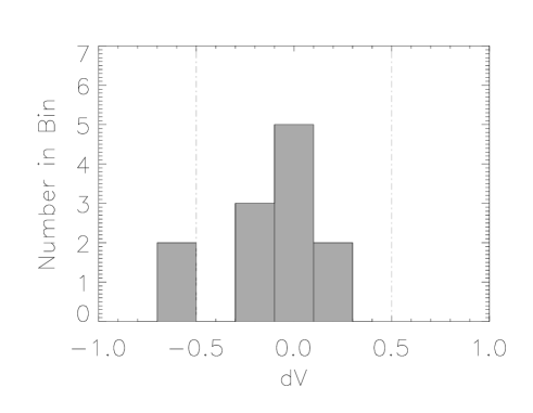
Figure 4: Histogram of $\delta V=(V_{\rm thick}-V_{\rm thin})/\Delta V_{\rm thin}$, where $V_{\rm thick}$ and $V_{\rm thin}$ were determined from the HCO${}^{+}(1-0)$ and H¹³CO${}^{+}(1-0)$ lines, respectively. The vertical dashed lines indicate the $\pm 5\sigma_{\delta V}$ level.

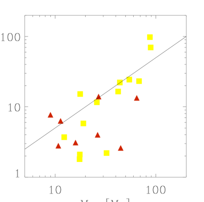
Figure 5: Total core mass, $M_{\rm core}=M_{\rm blast}$, vs. the virial mass, $M_{\rm vir}$, calculated using the velocity linewidths of the NH₃(1,1) and N₂H${}^{+}(1-0)$ transitions (see text). Yellow, filled squares represent proto-stellar cores and red, filled triangles represent starless cores. The solid line indicates the minimum $M_{\rm core}=0.5M_{\rm vir}$ for which the cores should be self-gravitating. Individual values of $M_{\rm vir}$ are listed in Table 7.

3.5.2 Virial mass

We then estimate the virial mass of the cores assuming they are simple spherical systems with uniform density (MacLaren et al. 1988):

$$M_{\rm vir}{\rm[M_{\odot}]}=210\,R_{\rm dec}{\rm[pc]}\,(\Delta V_{\rm av}{\rm[km\leavevmode\nobreak\ s^{-1}]})^{2}$$ (6)

where $R_{\rm dec}$ is the deconvolved source radius and $\Delta V_{\rm av}$ represents the line FWHM of the molecule of mean mass, calculated as the sum of the thermal and turbulent components:

$$\Delta V_{\rm av}^{2}=\Delta V_{\rm mol}^{2}+kT8\ln 2\,\left(\frac{1}{m_{\rm av}}-\frac{1}{m_{\rm mol}}\right)$$ (7)

where $\Delta V_{\rm mol}$ is the line FWHM of the molecular transition being considered and $m_{\rm av}=2.3$ amu is the mean molecular weight (with respect to the total number of particles), assuming a mass fraction for He of 25%. We note that according to MacLaren et al. (1988), Eq. (6) may lead to a mass overestimate if the density distribution is not uniform. For example, in the case of a sphere with a density distribution $\rho\propto r^{-2}$ the numerical factor in Eq. (6) should be replaced by 126.

As the deconvolved source radius we used the BLAST-derived values of Olmi et al. (2009). We decided to use the BLAST sizes, to estimate the virial masses, instead of the Mopra-derived sizes for two main reasons: (i) the linewidths are mostly measured from the single-point spectra of NH₃, and where NH₃ was not observed or not detected we used the observations of N₂H⁺, for which only a few maps were available; (ii) the BLAST maps are not affected by spatial variations that may instead affect specific molecules and thus likely give a better representation of the mass distribution in each source.

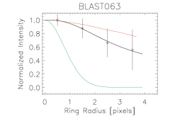
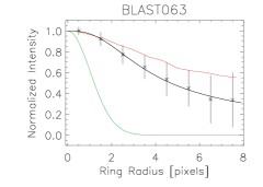
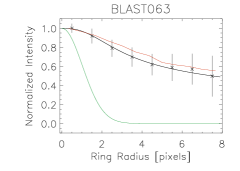
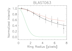
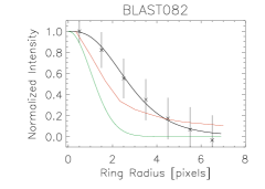
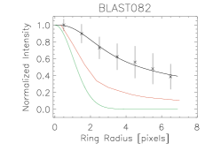
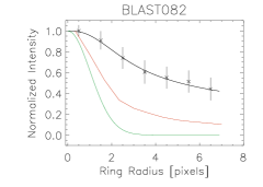
Figure 6: Examples of normalized radial profiles for sources BLAST063 (starless, top panels) and BLAST082 (proto-stellar, bottom panels). The points and error bars represent the ring-averaged integrated intensity in the molecular lines (from left to right) N₂H${}^{+}(1-0)$, HNC$(1-0)$, HCO${}^{+}(1-0)$ and HCN$(1-0)$. The black solid line represents the fit obtained using Eq. (8). The red solid line shows the radial profile of the averaged BLAST intensity at 250 $\mu$m, and the green solid line represents the 3-mm beam profile of the Mopra telescope. Each pixel corresponds to 15 arcsec.

As previously stated, the line FWHM is calculated from the NH₃(1,1) single-point spectra toward each source, if available, or from the N₂H${}^{+}(1-0)$ line otherwise, since these molecules are less likely to be affected by depletion, they trace the denser gas and are mostly optically thin. The linewidths determined by the fit procedure are artificially broadened by the velocity resolution of the observations, and thus we subtracted in quadrature the resolution width, $\Delta V_{\rm res}$, from the observed line FWHM, $\Delta V_{\rm obs}$, such that $\Delta V_{\rm mol}=\sqrt{\Delta V_{\rm obs}^{2}-\Delta V_{\rm res}^{2}}$.

Table 8: Parameters for fit to the radial profile of column density.

Source #		N2H+			HNC			HCO+			HCN
		$R_{flat}$	$\eta$		$R_{flat}$	$\eta$		$R_{flat}$	$\eta$		$R_{flat}$	$\eta$
		[arcsec]			[arcsec]			[arcsec]			[arcsec]
9		$-$	$-$		67.5	1.2		15.0	0.3		34.5	0.9
13		$-$	$-$		69.0	3.4		16.5	0.6		19.5	0.5
24		28.5	1.1		48.0	1.5		15.0	0.8		22.5	1.1
31		$-$	$-$		37.5	3.3		27.0	1.8		15.0	0.4
34		$-$	$-$		57.0	1.4		16.5	0.7		$-$	$-$
40		27.0	2.7		45.0	1.0		16.5	0.3		16.5	0.2
41		$-$	$-$		$-$	$-$		33.0	0.8		$-$	$-$
47		$-$	$-$		30.0	0.8		16.5	0.4		15.0	0.4
50		$-$	$-$		$-$	$-$		15.0	0.3		18.0	0.6
56		$-$	$-$		58.5	2.3		39.0	1.9		16.5	0.5
57		$-$	$-$		$-$	$-$		20.0	0.6		$-$	$-$
63		70.0	2.0		30.0	0.9		18.0	0.4		24.0	0.5
81		24.0	2.6		21.0	1.3		15.0	0.7		18.0	1.1
82A		31.5	2.4		22.5	0.7		16.5	0.5		21.0	0.5
82B		31.5	2.4		16.5	0.6		16.5	0.5		16.5	0.5
89		$-$	$-$		$-$	$-$		36.0	1.1		$-$	$-$
101		$-$	$-$		22.5	0.7		27.0	1.2		33.0	1.6
109		$-$	$-$		$-$	$-$		36.0	2.8		$-$	$-$

The resulting virial masses are listed in Table 7 and a plot of the total core mass, $M_{\rm blast}$, as derived from BLAST, vs. the virial mass is shown in Figure 5. We note that nearly all of the starless cores lie below the self-gravitating line, indicating that they are unlikely to be gravitationally bound, whereas more than half of the proto-stellar cores lie near or above that line, confirming that they are gravitationally bound (about 30% of all sources have $M_{\rm core}/M_{\rm vir}>0.5$). However, as we mentioned above, for a non-uniform density distribution (see Section 3.6), e.g. of type $\rho\propto r^{-2}$, all virial masses should be multiplied by a factor 0.6. In this case, most of the proto-stellar cores would move above the self-gravitating line and also most of the starless cores would be located near that line (about 60% of all sources have $M_{\rm core}/M_{\rm vir}>0.5$ in this case).

3.6 Radial profiles of column density

In order to identify significant differences in the distribution of both molecular gas and dust continuum, we have derived radial profiles of the column density from both the BLAST maps at 250$\,\mu$m and from the Mopra maps of the integrated intensity of the different molecular transitions. While the BLAST 500$\,\mu$m measurements would be somewhat less affected by optical depth effects, we have chosen to compare our molecular data to the BLAST 250$\,\mu$m measurements since they are closely matched to the Mopra beam.

Previous work has shown that single-power-law density, or column density, profiles do not fit the emission from dense cores and that a central flattening is always needed to reproduce the data (e.g., Tafalla et al. 2002 and references therein). Among the standard analytic profiles that combine the power-law behavior of column density for large radii $r$ and a central flattening at small $r$, is the following function:

$$N(r)=N_{\rm flat}\left[\frac{R_{\rm flat}}{(R_{\rm flat}^{2}+r^{2})^{1/2}}\right]^{\eta}$$ (8)

where the column density is approximately uniform, with $N\sim N_{\rm flat}$, for $r\ll R_{\rm flat}$, and it falls off as $r^{-\eta}$ for $r\gg R_{\rm flat}$.

In the fitting procedure we first circularly average the maps of the integrated intensity of selected molecular transitions around the peak, and then use a $\chi^{2}$ routine to fit the column density profile, obtained from the integrated intensity with Eq. (3), using the model given by Eq. (8), after convolution with a 2D $38^{\prime\prime}$ Gaussian. The procedure is then repeated for the BLAST250 maps. The column density profiles obtained from the spectral line maps and the dust continuum maps are then compared to find any possible evidence of chemical effects such as, for example, freezing-out on grains.

The results of the radial profile fits to individual sources are listed in Table 8, while in Table 9 we list the average values of the parameters $\eta$ and $R_{\rm flat}$, i.e. $\langle\eta\rangle$ and $\langle R_{\rm flat}\rangle$, obtained by selecting only fits to the radial profiles that converged. We can note several trends: first, apart from the large scatter observed in the case of the N₂H⁺ and HNC molecules, the $\langle R_{\rm flat}\rangle$ values are quite consistent within the errors. Second, the value of $\langle\eta\rangle$ for the N₂H⁺ molecule is significantly higher compared to the other molecules although, once again, the HNC molecule shows a larger scatter. We tentatively note a trend of decreasing $\langle\eta\rangle$ values from HNC to HCO⁺ and then HCN, but given the errors this cannot be considered significant. We also note that the large uncertainty in the $\langle R_{\rm flat}\rangle$ value for N₂H⁺ is due to the BLAST063 source. If this source is not included, then we would have $\langle R_{\rm flat}[{\rm N_{2}H^{+}}]\rangle=28.5\pm 3.2$, quite close to the values estimated for HCN and HCO⁺.

As a final trend, when comparing the radial profiles obtained by the BLAST dust continuum with those of the molecular tracers, Figure 6 shows that, at least for the two cores shown in the figure, the agreement between the radial profiles of the molecular tracers and of the dust continuum is better for the starless core (BLAST063). In order to get a quantitative comparison, we have applied the two-sample Kolmogorov-Smirnov test (K-S test) to the BLAST- and Mopra-derived radial profiles. The K-S test evaluates the maximum deviation between the cumulative distribution functions of the two data sets and also the associated probability, $p_{\rm ks}$ ($0<p_{\rm ks}<1$), that two arrays of data values are drawn from the same distribution. Small values of $p_{\rm ks}$ show that the cumulative distribution function of one data set is significantly different from the other. For the two sources shown in Figure 6 we get an average value of $p_{\rm ks}=0.66$ for BLAST063 and $p_{\rm ks}=0.24$ for BLAST082, confirming that in BLAST063 the dust and molecular gas radial profiles are more similar than in BLAST082.

However, it is clear comparing the radial profiles and also the integrated intensity maps, that the starless cores have a wider range of morphologies, with sources showing a good agreement between the dust continuum and the molecular radial profiles (although not necessarily in all molecular tracers, e.g., in sources BLAST013 and BLAST031), and sources where this agreement is less evident (e.g., in BLAST056 and BLAST063). These differences suggest that the starless sources in our sample are currently in different evolutionary phases.

Table 9: Average properties of radial profiles.

Spectral line	$\langle R_{\rm flat}\rangle$	$\langle\eta\rangle$	$\langle X_{\rm mol}\rangle$
	[arcsec]
N2H${}^{+}(1-0)$	$35.4\pm 17.2$	$2.24\pm 0.65$	$(7.3\pm 5.4)\,\times 10^{-11}$
HNC$(1-0)$	$40.4\pm 18.3$	$1.39\pm 1.00$	$(4.5\pm 2.9)\,\times 10^{-10}$
HCO${}^{+}(1-0)$	$21.9\pm 8.6$	$0.87\pm 0.67$	$(1.3\pm 0.8)\,\times 10^{-9}$
HCN$(1-0)$	$20.8\pm 6.4$	$0.68\pm 0.39$	$(0.8\pm 1.2)\,\times 10^{-9}$
NH3	$-$	$-$	$(1.7\pm 3.1)\,\times 10^{-7}$

Figure 7: Source-averaged radial profiles of the relative molecular abundances (from left to right) of [HCO⁺]/[HCN], [HNC]/[HCN] and [N₂H⁺]/[HCO⁺]. The abundances are normalized with respect to the peak value. The top and bottom panels show the resulting averages for all starless and proto-stellar cores, respectively, where data were available. Pixel size as in Figure 6.

4 Discussion

In this section we will describe how the results obtained in Section 3 allow us to determine the relative molecular abundances, and in particular how these abundances vary as a function of the radial distance in both starless and proto-stellar cores. We will also discuss how the relative molecular abundances can be used to roughly estimate the chemical evolutionary status of the sources. In the last part of the section we will analyze the degree of correlations among various physical and chemical parameters, which will also allow to highlight further differences between starless and proto-stellar cores.

4.1 Determining molecular abundances

As we mentioned earlier, we have estimated the molecular abundances by comparing the molecular gas mass, $M_{\rm cd}$, with the total gas mass, $M_{\rm blast}$, estimated by the BLAST measurements of the dust continuum, i.e., $X_{\rm mol}=M_{\rm cd}/M_{\rm blast}$. We prefer this method to the alternative technique of obtaining $X_{\rm mol}$ by means of a pixel-by-pixel comparison of the column densities in the Mopra and BLAST maps, which could be affected by differences in the spatial distribution of the spectral line and dust continuum emission. The estimated abundances are shown in Table 10 and their average values are listed in Table 9. The large uncertainties in the estimated abundances are likely the consequence of uncertainties in the derivation of the BLAST masses, of the different spatial distribution of the molecular gas and the dust, and possibly also of different chemical evolutionary phases (see the discussion in Sections 4.2 and 4.3).

The average value of $X({\rm N_{2}H^{+}})=(7.3\pm 5.4)\,10^{-11}$ listed in Table 9 is consistent with that found by, e.g., Blake et al. (1995) in NGC1333 and also by Zinchenko et al. (2009) in S187 and W3. However, it is relatively low compared to mean values found in other cloud cores. For example, Womack et al. (1992) and Benson et al. (1998) found mean values of $X({\rm N_{2}H^{+}})$ of $4\times 10^{-10}$ and $7\times 10^{-10}$, respectively, from various samples.

From Table 9, we can also determine the average values of some relative abundances: $X({\rm HCN})/X({\rm HNC})\sim 1.8$, $X({\rm HNC})/X({\rm HCO^{+}})\sim 0.3$, and $X({\rm HCN})/X({\rm HCO^{+}})\sim 0.6$. The value of $X({\rm HNC})/X({\rm HCO^{+}})$ agrees reasonable well with that estimated by Godard et al. (2010) ($0.5\pm 0.3$), whereas the other two relative abundances, $X({\rm HCN})/X({\rm HNC})$ and $X({\rm HCN})/X({\rm HCO^{+}})$ both appear to be somewhat lower compared to the estimated values ($4.8\pm 1.3$ and $1.9\pm 0.9$, respectively) of Godard et al. (2010), though all estimates have large ($\ga 50$%) uncertainties.

Figure 8: Column density correlations for the same molecules examined in Figure 7. The solid line represents the linear fit (from Bayesian statistics, see text) to all points. The Spearman rank coefficient is $>0.5$ in all three cases, with a peak of 0.75 in the plot of $N({\rm HNC})$ vs. $N({\rm HCN})$.

Table 10: Abundance estimates.

Source #	N2H+	HNC	HCO+	HCN	NH3
	[$\times 10^{-9}$]	[$\times 10^{-9}$]	[$\times 10^{-9}$]	[$\times 10^{-9}$]	[$\times 10^{-8}$]
9	$-$	0.85	0.50	0.09	25.4
13	$-$	0.57	1.18	0.54	$-$
24	0.06	0.26	0.55	0.18	0.6
31	$-$	$-$	0.56	0.16	96.9
34	$-$	0.47	0.41	$-$	$-$
40	0.02	0.78	0.22	0.40	3.3
41	$-$	$-$	2.63	$-$	2.7
47	$-$	0.86	1.03	2.21	18.3
50	$-$	$-$	2.59	4.3	$-$
56	$-$	0.07	0.84	0.33	$-$
57	$-$	$-$	0.62	$-$	$-$
63	0.11	0.35	0.77	0.62	6.7
81	0.03	0.19	0.58	0.20	0.08
82	0.15	0.49	1.8	0.26	0.9
89	$-$	$-$	2.80	$-$	$-$
101	$-$	0.46	1.65	0.44	$-$
109	$-$	$-$	0.89	$-$	$-$

4.2 Radial profiles of relative molecular abundances

The computation of the absolute molecular abundances is affected by our ability to determine the mass distributions of both a specific molecular tracer and of the total mass. In particular, the spatial distribution (i.e., pixel-by-pixel) of the total mass, as determined from the dust continuum, is seriously affected by our ability to estimate and subtract the local background emission.

In order to avoid these difficulties, we have decided to evaluate only the spatial distribution of the relative molecular abundances, which depend solely on our Mopra observations and are not affected by variable levels of background in the bolometers maps. In Figure 7 we show the source-averaged, radial profiles of the normalized relative abundances [HCO⁺]/[HCN], [HNC]/[HCN] and [N₂H⁺]/[HCO⁺] with associated standard-deviations. We show separately the resulting averages for proto-stellar and starless cores with available map data. For each separate source, the relative abundances are normalized with respect to the observed maximum value, as a function of radius. We then take the median values of these normalized relative abundances in each sub-sample of sources. The advantage of using the normalized values is to be less affected by the variations of the absolute values of the abundances from source to source, and highlights instead the behaviour of the abundances as a function of radius.

Therefore, in Figure 7 we note that while in the proto-stellar cores the [HCO⁺]/[HCN] ratio peaks at the center of the sources, in the starless cores the peak is slightly off-center. This shows that on average the abundance of [HCO⁺] relative to that of [HCN] is somewhat lower toward the center of the starless cores. As far as the [HNC]/[HCN] ratio is concerned, our data show that this relative abundance is quite flat in both starless and proto-stellar cores, though a slight decrease as a function of radius can be observed, particularly toward proto-stellar cores. Finally, we can note the very different behaviour of the [N₂H⁺]/[HCO⁺] ratio in starless and proto-stellar cores. In fact, while in the former this abundance ratio is quite flat, in proto-stellar cores the [N₂H⁺]/[HCO⁺] ratio can be observed to decrease toward larger radii.

A detailed comparison of these radial profiles with simulations obtained using recent chemical models (e.g., Lee et al. 2004, Aikawa et al. 2008), which follow the chemical evolution of a source both as a function of time and of radial position, is difficult because they usually model the chemistry of the source only out to a radius $\sim 1-2\times 10^{4}\,$AU, a size lower than that (26600 AU) covered by the Mopra beam at the distance of Vela-D.

However, we note that some features present in Figure 7 are consistent with, e.g., the model of Lee et al. (2004). The faster drop-off at large angular radii of the radial profile of the [N₂H⁺]/[HCO⁺] ratio in proto-stellar cores is consistent with the molecular abundance profiles after collapse discussed by Lee et al. (2004), though they are not consistent with similar radial profiles discussed by Aikawa et al. (2008). Also, the fact that in Figure 7 the peak of the [HCO⁺]/[HCN] ratio in starless cores is slightly off-center could be a consequence of HCO⁺ depletion, which is more effective in decreasing the column density of HCO⁺ toward the center of the sources and is more effective at earlier times. In fact, Lee et al. (2004) have shown that depletion initiates during the pre-collapse phase and proceeds through the collapse of the source.

4.3 Chemical status of the cores

In this section we further discuss some chemical implications of the relative molecular abundances. It is often found in the literature that some molecules are classified either as “early-time” ($10^{4}-10^{6}$ years after the onset of chemistry) or “late-time” species (maximum abundances reached at steady state, after $10^{6}-10^{8}$ years of chemical evolution), based on the production pathways via ion$-$molecule or neutral$-$neutral reactions. Of the molecules discussed here HCO⁺ and NH₃ are usually considered as late-time molecules, but the situation of HCN and HNC is less clear in this picture.

However, we can attempt to use the [HNC]/[HCN] abundance ratio as a measure of the evolutionary phase and temperature in our sources. In fact, converting Figure 7 into absolute values (instead of the normalized values shown in the figure) for the relative molecular abundances we find that: (i) the abundances of HCN and HNC are not significantly different between the proto-stellar and the starless cores, thus a systematic change in the HCN abundance due to chemical evolution is not apparent in this study; (ii) the average [HNC]/[HCN] ratio is in agreement with the values measured in 19 low-mass starless and proto-stellar cores by Hirota et al. (1998).

Figure 9: Median core size (left panels) and median linewidth, $\Delta V$ (right panels) vs. $n_{\rm eff}$ (at 15 K), shown separately for a sub-sample of proto-stellar (top row) and starless (bottom row) cores. The plot of $\Delta V$ vs. $n_{\rm eff}$ makes use of the single-point observations, instead of spectral line maps as in the left panels, allowing for more molecular lines to be used. The effective densities are listed in Table 2. The plot also includes some detections of the HC₃N$(1-0)$ line, with $n_{\rm eff}=2.5\times 10^{4}$. The solid line represents the linear fit (from Bayesian statistics) to all points.

According to gas-phase chemical models, HCN and HNC are mainly produced by a dissociative recombination reaction of the HCNH⁺ ion with an electron (see Hirota et al. 1998 and references therein):

$${\rm HCNH^{+}+e^{-}}\rightarrow\left\{\begin{array}[]{l}{\rm HCN+H}\\ {\rm HNC+H}\\ \end{array}\right.$$ (9)

The branching production ratio of HCN, $\alpha$, is defined as [HCN]/[HNC]$=\alpha/(1-\alpha)$, if $T_{k}\ll T_{c}$, where $T_{c}\simeq 24\,$K is the threshold temperature above which neutral$-$neutral reactions dominate the [HCN]/[HNC] ratio. If we take a median value of [HCN]/[HNC]$\simeq 1$ in our cores, the branching production ratio of HCN is estimated to be $\alpha\simeq 0.5$, somewhat higher than the value reported by Hirota et al. (1998) ($\alpha\simeq 0.4$), but in agreement with the range of values found by Nikolić et al. (2003) toward L1251 ($\alpha\simeq 0.2-0.8$). The relatively low value of $\alpha$ suggests that the more energetic paths for destruction of HNC, once the temperature of the gas exceeds the critical temperature, are less favorable, and thus it constitues a further indirect evidence that our cores are cold.

Another parameter to assess the chemical status of our cores is the [N₂H⁺]/[H¹³CO⁺] abundance ratio. Fuente et al. (2005) have proposed this ratio as a measure of the evolutionary phase of a source. According to these authors, since the abundance of N₂H⁺ tends to remain constant in starless clumps, while H¹³CO⁺ could suffer from depletion in the densest part, then the [N₂H⁺]/[H¹³CO⁺] ratio could be used as an indication of the chemical evolutionary phase of the cores. If we use the single-point observations of both N₂H⁺ and H¹³CO⁺ we find a median value of their relative abundance, [N₂H⁺]/[H¹³CO⁺]$=5.7\pm 1.9$, which is intermediate in the range of values proposed by Fuente et al. (2005) spanning from Class 0 objects (where molecular depletion is significant and the [N₂H⁺]/[H¹³CO⁺] ratio is maximum, $\sim 15$) to more evolved objects where the ratio is minimum ($\sim 3$). Note, however, that the objects studied by Fuente et al. (2005) are on average more evolved than those in our sample of cores in Vela-D.

4.4 Correlations between parameters

4.4.1 Column density correlations

We can use the molecular column densities estimated in the previous sections to compare the behavior of the molecules. If we analyze molecules with different critical densities, we would expect their molecular transitions to be emitted in different volumes of gas, in the presence of density gradients. Likewise, molecules with similar critical densities will be excited in the same volume of gas, in the absence of strong abundance gradients.

We performed this test only in those sources where spectral line maps were available, to ensure that we integrate over all molecular emission. Thus, in these correlation plots all information about the specific spatial distribution of the different molecular tracers is lost. In addition, the inclusion in this analysis of spectral line maps only, dramatically decreases the size of the sample, which also represents a range of masses, chemistries, and evolutionary states.

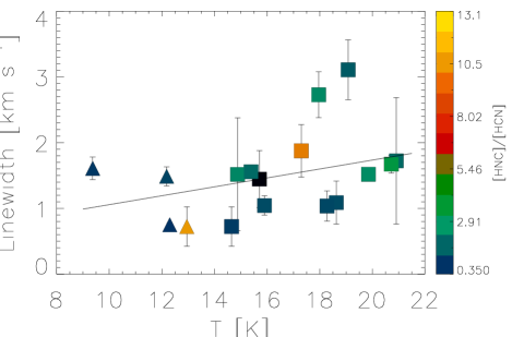
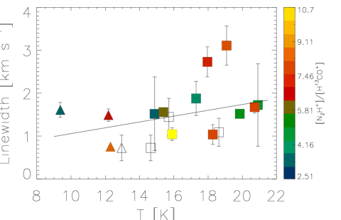
Figure 10: Plot of average linewidth vs. core temperature. The BLAST-derived dust temperature has been used, except in those sources where $T_{\rm k}$ could be determined from NH₃ (see Section 3.3). In estimating the averages, only the linewidths of the optically thin molecular tracers (N₂H⁺, H¹³CO⁺ and H¹³CN) have been considered. The triangles and squares represent starless and proto-stellar cores, respectively. The filling color code represents the relative abundance [HNC]/[HCN] (top panel) and [N₂H⁺]/[H¹³CO⁺] (bottom panel). The solid line represents the linear fit (from Bayesian statistics) to all points.

Our results are presented in Figure 8, where we have used the Bayesian IDL routine LINMIX_ERR to perform a linear regression, to find the slope of the best fit line in each case. In the top panel we plot the column density of HCO⁺ vs. the column density of HCN. HCN should be a higher-density gas tracer, compared to HCO⁺; however, despite a considerable scatter, the two column densities show a modest correlation, with a Spearman rank coefficient $>0.5$. The column densities of HCN and its isomer HNC also appear to be well correlated (correlation coefficient $=0.75$) in the middle panel of Figure 8. Finally, in the bottom panel, we also compare the column densities of the chemically opposite species N₂H⁺ and HCO⁺. The few points in this panel are a consequence of the fewer available maps for N₂H⁺ compared to the other molecular tracers. However, we still see a correlation between the two column densities (correlation coefficient $>0.5$).

The variable degree of correlation and the scatter in Figure 8 is an indication of source-to-source variations in the physical and chemical conditions. However, these qualitative trends are remarkable given the diversity of our sources and relatively small sample size.

4.4.2 Correlations with $n_{\rm eff}$

The molecular transitions observed by us are characterized by a range of critical densities, thus allowing us to examine how specific physical parameters change as a function of the gas traced by a specific line. However, instead of using the critical density, $n_{\rm crit}$, in our analysis we prefer to use the effective density, $n_{\rm eff}$, to characterize the volume of gas where a given spectral line is generated. As discussed in Evans (1999), the ability to detect a transition is usually associated with a number density larger than $n_{\rm crit}$, but lines are also easily excited in subthermally populated gas with densities more than an order of magnitude lower than $n_{\rm crit}$.

To account for effects such as optical depth, multilevel excitation effects, and trapping, we use the definition of Evans (1999), where $n_{\rm eff}$ represents the density needed to excite a $T_{R}=1\,$K line (where $T_{R}$ is the observed radiation temperature) for a given kinetic temperature, as calculated with a non-LTE radiative transfer code. We specifically calculated the effective densities of our molecular tracers by using the online version of RADEX (van der Tak et al. 2007), a non-LTE radiative transfer code, assuming $\log(N/\Delta v)=13.5\,$cm${}^{-2}/($km s${}^{-1})$ (see Evans 1999) and a kinetic temperature of 15 K for all species (see Table 2).

Figure 9 shows the (deconvolved) core diameter, as determined from the molecular intensity maps, as a function of $n_{\rm eff}$. The observed core diameter is estimated using the area enclosed within the half-peak intensity contour and then deconvolved using the standard Gaussian deconvolution with the Mopra beam. We then take the median value of the size (using the selected sources listed in Figure 9) and plot it as a function of $n_{\rm eff}$ in Figure 9, where the error bars represent the median absolute deviations. By comparing the values of the measured core diameter in starless and proto-stellar cores we note that for the same value of $n_{\rm eff}$ the starless cores have on average a larger size.

Table 11: Median properties of starless and proto-stellar cores.

Source Type	$R_{\rm flat}$	$\eta$	FWHM	$T$	$\frac{M_{\rm core}}{M_{\rm vir}}$	$\frac{P_{\rm tot}}{k}$	$\frac{\rm[NH_{3}]}{\rm[N_{2}H^{+}]}$	$\frac{\rm[N_{2}H^{+}]}{\rm[H^{13}CO^{+}]}$
	[arcsec]		[km s-1]	[K]		[$\times 10^{6}\,$cm-3 K]
Starless	$27.0\pm 12.0$	$0.8\pm 0.7$	$1.4\pm 0.4$	$15.1\pm 1.6$	$0.5\pm 0.3$	$\sim 5$	$\sim 10^{3}$	$5.7\pm 1.7$
BLAST063	$24.0\pm 6.0$	$0.6\pm 0.3$	$1.5\pm 0.1$	12.2	0.3	$\sim 10$	$\sim 600$	$5.7$
Proto-stellar	$21.0\pm 5.9$	$1.1\pm 0.5$	$1.6\pm 0.6$	$16.8\pm 1.8$	$0.8\pm 0.4$	$\sim 19$	$\sim 60$	$6.4\pm 1.9$

Figure 9 also shows the source linewidth, $\Delta V$, measured from single-point spectra, as a function of $n_{\rm eff}$. Because in this case we are using the single-point observations, we could include in the plot almost all molecular transitions listed in Table 2. Furthermore, since linewidths may be broadened by optical depth effects, for Figure 9 we selected only those source/line cases with $\tau<1$. We note that no significant difference in $\Delta V$ is observed, for the same value of $n_{\rm eff}$, between proto-stellar and starless cores, but we find that in starless cores $\Delta V$ and $n_{\rm eff}$ are correlated. In fact, as for the case of Figure 8 we have used the IDL routine LINMIX_ERR to perform a linear regression, and we find a Spearman rank coefficient of 0.97 for the starless cores. However, this correlation coefficient drops to 0.23 for the proto-stellar cores.

4.4.3 Linewidth-temperature correlation

Since there is no single measurement that can determine the “exact” evolutionary stage of each source, as a further test to help estimate the status of the cores in our sample we plot in Figure 10 the linewidth vs. the core temperature. In order to avoid possible optical thickness effects, the figure only includes the linewidths of the (mostly) optically thin molecular tracers, i.e., N₂H⁺ and the two isotopologues H¹³CO⁺ and H¹³CN. From this plot we also had to eliminate those sources with a poor determination of the linewidths because of weak lines and/or noisy spectra.

Figure 10 thus shows that there is a clear segregation in temperature between starless and proto-stellar cores. The figure also shows that there is a modest correlation between linewidth and temperature. As for the case of Figure 8 we have used the IDL routine LINMIX_ERR to perform a linear regression, and we find a Spearman rank coefficient of 0.47. This modest correlation is confirmed by the fact that the median values of the linewidth determined for the starless and proto-stellar cores are $1.4\pm 0.4$ and $1.6\pm 0.6$ km s^-1, respectively (see Table 11), which are consistent within the errors.

Figure 10 also encodes the information about the relative molecular abundances [HNC]/[HCN] and [N₂H⁺]/[H¹³CO⁺], discussed in Section 4.3. No apparent trend of [HNC]/[HCN] or [N₂H⁺]/[H¹³CO⁺] with either linewidth or temperature can be seen.

4.5 Comments to specific sources mapped with the Mopra telescope

In this section we further discuss some starless and proto-stellar cores that have been mapped at Mopra, including the “transition” source BLAST063.

BLAST024. This source is a compact proto-stellar core, where the spatial distribution of the emission of all main tracers observed by us is centered on the BLAST dust core. Wing emission is detected in the single-point HCO${}^{+}(1-0)$ spectrum, suggesting the presence of a molecular outflow. However, due to the low SNR in our maps, we could not produce an image of the outflow, as it is the case also for sources BLAST081 and BLAST082.

BLAST031. This is a moderately compact starless core, where the HCN$(1-0)$ and HCO${}^{+}(1-0)$ emission trace quite well the BLAST continuum emission, but the HNC$(1-0)$ emission is seen to peak at an offset position compared to the BLAST emission and the other two molecular probes. Such offsets are also found toward other sources (see below).

BLAST034. This is an irregularly shaped, starless core which shows two well separated velocity components in the single-point HCO${}^{+}(1-0)$ spectrum, with the main (mapped) component being the low-velocity one ($\simeq 2\,$km s^-1). The two velocity components are also detected in the HNC$(1-0)$ spectrum.

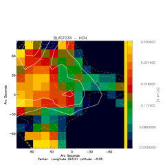
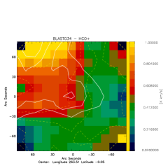
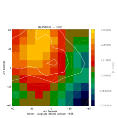
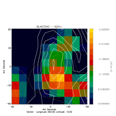
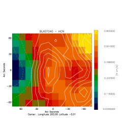
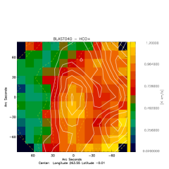
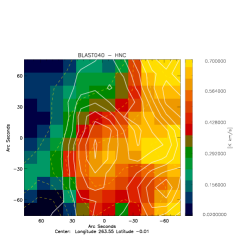
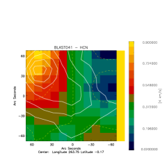
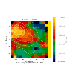
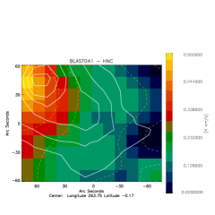
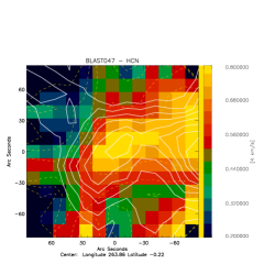
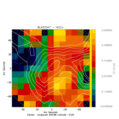
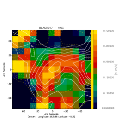
Figure 12: Same as Figure 11 for sources BLAST034, BLAST040, BLAST041 and BLAST047.

BLAST047. This source also shows a double-peaked HCO${}^{+}(1-0)$ spectrum. However, both the channel map of the HCO${}^{+}(1-0)$ emission and the spatial distribution of the HNC and HCN$(1-0)$ emission (see Figure 12) suggest that HCO⁺ is self-absorbed at the position of the BLAST peak. One can also note that HCN, and especially HNC, trace very well the BLAST contour plots.

BLAST063. This source is the most intense starless core mapped by us at Mopra. This core has been classified throughout this paper and was originally classified as starless by Olmi et al. (2009) because no MIPS compact source at 24$\,\mu m$ could be found at its location. However, we have found that the single-point HCO${}^{+}(1-0)$ spectrum shows line-wing emission, indicating the presence of a molecular outflow, which should actually change the source type from starless to proto-stellar. The fact that no 24$\,\mu m$ emission is detected toward this core, though a molecular outflow is already active, suggests that the proto-stellar core has just formed and is thus in an earlier stage compared to BLAST024, BLAST081 and BLAST082. Therefore, this core could tentatively be classified as being in a “transition phase” from starless to proto-stellar. We also note that this source has an elongated shape, and we can see that the HCN$(1-0)$ and HNC$(1-0)$ emission trace very well the BLAST continuum emission, whereas there is an offset between the HCO${}^{+}(1-0)$ emission and the dust emission.

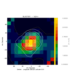
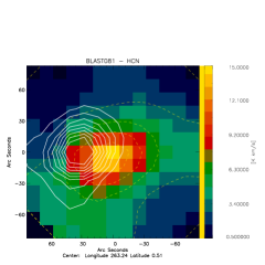
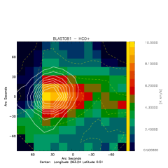
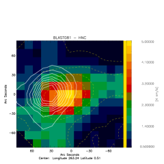
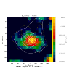
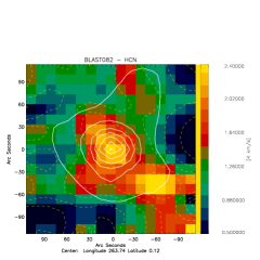
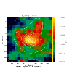
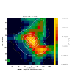
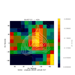
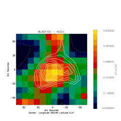
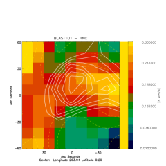
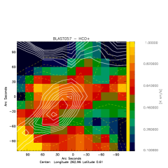
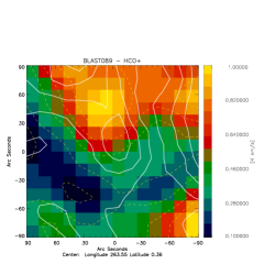
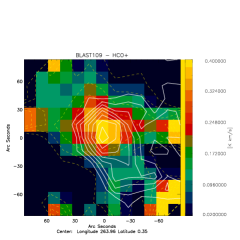
Figure 14: Same as Figure 11 for sources BLAST081, BLAST082 and BLAST101. The bottom row shows the HCO${}^{+}(1-0)$ integrated intensity maps of sources BLAST057, BLAST089 and BLAST109.

BLAST081. This source is another compact proto-stellar core mapped with the Mopra telescope. Despite some artefacts visible in the HCO${}^{+}(1-0)$ map (see Figure 14) we note that while the N₂H${}^{+}(1-0)$ and (possibly) HCO${}^{+}(1-0)$ emission follow closely the BLAST continuum emission, the emission of the two isomers HCN and HNC peak at an (identical) offset position compared to the BLAST maximum. This is the only example of such an offset observed among the three proto-stellar cores mapped with the Mopra telescope, though it is also partly observed toward the early proto-stellar core BLAST063. Since our sensitivity was not high enough to map the optically thin isotopologues, such as H¹³CO⁺ and H¹³CN, we cannot determine at present whether this offset is due to optical depth effects or chemical variations. As in BLAST024, the HCO${}^{+}(1-0)$ spectrum shows line-wing emission, indicating the presence of a molecular outflow.

BLAST082. This source is the third compact proto-stellar core mapped at Mopra. Contrary to BLAST081, all mapped molecular tracers are well centered on the BLAST continuum emission and also follows quite well the less dense material. However, the HCN$(1-0)$ and HNC$(1-0)$ maps show an additional smaller core, located at $(\Delta l,\Delta b)\simeq(-60^{\prime\prime},-60^{\prime\prime})$ (see Figure 14), which is not visible in the HCO${}^{+}(1-0)$ map. This sub-structure may be a consequence of core fragmentation and the difference observed in the various molecular tracers may indicate a different chemical status compared to the main core. Then, like BLAST034 and BLAST047, the single-point HCO${}^{+}(1-0)$ spectrum is also double-peaked, but the channel map suggests this is the consequence of two velocity components aligned along the line of sight. Like BLAST024 and BLAST081 the HCO${}^{+}(1-0)$ spectrum also suggests the presence of a molecular outflow. Line wings in the HCO${}^{+}(1-0)$ spectrum are also observed toward other sources, as listed in Table 15.

4.6 Median properties of starless and proto-stellar sources and comparison with other surveys

In this section we summarize the main differences between starless and proto-stellar cores, by presenting a list of their median properties in Table 11. For comparison, we have also included source BLAST063 which we have defined as a transition source between the two classes of objects. One can note that the starless cores appear to be moderately colder and less turbulent compared to the proto-stellar sources, though the differences are within the uncertainties. The linewidths have been averaged among all optically thin tracers (N₂H${}^{+}(1-0)$, H¹³CO${}^{+}(1-0)$ and H¹³CN${}^{+}(1-0)$) and all sources. The lower temperature of the starless cores is simply a consequence of the analysis carried out by Olmi et al. (2009), but we now find that also their linewidths do not strongly differ from those of the proto-stellar cores.

We do find a more significant difference between starless and proto-stellar cores when we consider the radial profiles of the column densities. By using the results of Section 3.6 the median values of the parameters $R_{\rm flat}$ confirm that the proto-stellar cores are more compact on average. The parameter $\eta$, on the other hand, is subject to larger uncertainties, also due to our relatively low spatial resolution at the distance of Vela-D, and no definitive statement can thus be made. We note that the larger $R_{\rm flat}$ measured toward the starless cores agrees well with the conclusion of Caselli et al. (2002). In fact, these authors found that while proto-stellar cores in their sample (which includes sources from various star forming regions) were better modeled with single power-law density profiles, the starless cores presented a central flattening in the integrated intensity profile.

In terms of the kinematics of the cores, our findings are also very similar to those of Caselli et al. (2002). In fact, we find an average value for the velocity gradient in our sample (from the HCO⁺ results listed in Table 6) of $1.4\pm 0.3\,$km s^-1 pc^-1, and we do not find significant differences between starless and proto-stellar cores. This is consistent with the typical value of $2\pm 1\,$km s^-1 pc^-1 found by Caselli et al. (2002) in their sample. In terms of the equilibrium status of the cores, Caselli et al. (2002) found that their “excitation mass” to virial mass ratio is typically $M_{\rm ex}/M_{\rm vir}\simeq 1.3$, for both classes of cores. From Table 11, on the other hand, we can see that both starless and proto-stellar cores have $0.5\la M_{\rm core}/M_{\rm vir}\la 1$. Therefore, while the $M_{\rm core}/M_{\rm vir}$ ratio is somewhat lower compared to the results of Caselli et al. (2002) (but this may also be a consequence of the different methods to calculate the core masses) it is still very near or beyond the self-gravitating threshold of 0.5. We also find that in proto-stellar cores the $M_{\rm core}/M_{\rm vir}$ ratio is slightly larger than in starless cores, though they are still consistent within the errors.

In Table 11 we have also included the median values of the average total internal pressure (not the edge pressure), $P_{\rm tot}$, of each core in Vela-D for which we have measured (optically thin) linewidths. The values of $P_{\rm tot}$ have been calculated following the method described by Olmi et al. (2010) and are given in the usual cm^-3 K units for $P_{\rm tot}/k$. We note that in proto-stellar cores the median internal pressure is much higher than in starless cores, as expected. However, the confinement of the cores is of concern only for those sources (mostly starless) that are gravitationally unbound. Therefore, the starless cores which are gravitationally unbound according to the $M_{\rm core}/M_{\rm vir}$ ratio can be stable (against expansion) only if their edge pressure is less than the local ambient pressure (of order $P_{\rm ext}/k\sim 5\times 10^{5}\,$cm^-3 K in Vela-D, see Olmi et al. 2010). Pressure confined cores have been previously discussed, for example, by Lada et al. (2008) and Saito et al. (2008). Alternative sources of support could come from the magnetic field (see Olmi et al. 2010 and references therein), or the gravitationally unbound cores must otherwise be transient structures.

As far as chemical properties are concerned, Table 11 shows that the values of the relative abundance [N₂H⁺]/[H¹³CO⁺] for the starless and proto-stellar cores are quite similar. Thus, as noted in Section 4.3 we do not find any trend based on this ratio, as it has been suggested by Fuente et al. (2005). However, in Table 11 we note that the [NH₃]/[N₂H⁺] abundance ratio is significantly larger toward starless cores, though we had only two starless cores where we could effectively measure this ratio. This trend, if not the quantitative difference between the two classes of objects (because of the low statistics), is consistent with the findings of Friesen et al. (2010), who concluded that the relative fractional abundance of NH₃ to N₂H⁺ remains larger toward starless cores than toward protostellar cores by a factor of $\sim 2-6$.

These properties, and in particular the fact that many of the starless cores are gravitationally bound (hence, pre-stellar), suggest that at least most of the pre-stellar cores observed by us are indeed the precursors of the proto-stellar cores and not just transient objects following a different evolutionary path. Their similar median temperature and linewidths indicate that the envelopes of the sources have not had enough time to “register” the emergence of a protostar inside the core. In turn, this also means that most of the turbulence in the proto-stellar cores observed by us is generated prior to the appearance of a warm object inside the core.

Therefore, it appears that the transition from the pre- to the proto-stellar phase is relatively fast, leaving the core envelopes with almost unchanged physical parameters. Alternatively, if most proto-stellar cores observed had not had much time to evolve after the appearance of a protostar, this might also explain the similar median temperatures and linewidths of the two source types. However, the latter hypothesis seems less likely given that among our selected proto-stellar cores are also sources relatively evolved (see Olmi et al. 2009 and references therein).

In this respect, despite the uncertainties it is of interest to note that the values of the parameters $R_{\rm flat}$, $\eta$ and FWHM of source BLAST063 are somewhat intermediate between those of starless and proto-stellar cores. But, if the transition phase from pre- to proto-stellar is indeed fast, then one should not expect to detect many such transition objects, and their properties may be indistinguishable from those of either class of sources. More systematic observations of larger samples of sources are required to further study this issue.

5 Summary and conclusions

We presented 3-mm molecular line observations of the Vela-D region obtained with the 22-m Mopra radio telescope and 1.3 cm NH₃ observations carried out with the Parkes antenna. In total 8 molecular lines were analyzed in 40 sources, both starless and proto-stellar cores, previously detected by BLAST. A total of 20 spectral line maps were obtained. The results of our study can be summarized as follows:

1. Our spectral line maps show a wide variety of morphological types: very early and cold starless cores appear to have an irregular shape (e.g., BLAST009) in most or all molecular tracers mapped at Mopra. Some warmer cores (e.g., BLAST031) and cores at the transition phase from starless to proto-stellar (BLAST063) appear to be more regularly shaped and more compact. Finally, proto-stellar cores all show a more rounded shape and narrow radial intensity profiles.

2. We compared the kinetic temperature, $T_{\rm k}$, derived from the NH₃(1,1) and (2,2) observations, with the BLAST-derived dust temperature, $T_{\rm d}$, and found that the median value of their ratio is $T_{\rm k}/T_{\rm d}=1.2\pm 0.2$.

3. We found that all proto-stellar sources, and at least 7 starless cores mapped at Mopra, show velocity gradients. In two of the proto-stellar cores the direction of the velocity gradients measured in HNC and HCO⁺ are significantly different, suggesting the possibility that different systematic motions are simultaneously present (one of which likely is a molecular outflow).

4. The analysis of the virial masses showed that nearly all of the starless cores have masses below the self-gravitating threshold, indicating that they are unlikely to be gravitationally bound, whereas more than half of the proto-stellar cores have masses which are near or above the self-gravitating critical value. If a density profile closer to the one actually observed is considered in the calculation of the virial masses, then also most starless cores turn out to have masses near or above the self-gravitating threshold.

5. The average internal pressure of proto-stellar cores is higher than in starless cores, and both are higher than the typical ambient pressure in Vela-D. Cores (mostly starless) not gravitationally bound cannot thus be pressure-confined like, for example, the cores in the Pipe nebula.

6. The radial profile of the ring-averaged integrated spectral line intensity confirmed that proto-stellar cores have on average a more compact structure. We also found that the radial profile of the N₂H${}^{+}(1-0)$ emission falls-off more quickly, on average, than that of the C-bearing molecular lines HNC$(1-0)$, HCO${}^{+}(1-0)$ and HCN$(1-0)$.

7. We find a variable degree of correlation, with a significant scatter, between the column densities of chemically different molecular species, and also between molecular tracers with different effective densities. We also find that in starless cores the linewidth and effective density are well correlated. Instead, linewidth and temperature are not strongly correlated.

8. The branching production ratio of HCN and also the relatively low [N₂H⁺]/[H¹³CO⁺] abundance ratio confirm that all cores in our sample are cold and are on average in early evolutionary phases.

9. An analysis of the median properties of the starless and proto-stellar cores suggests that the transition from the pre- to the proto-stellar phase is relatively fast, leaving the core envelopes with almost unchanged physical parameters.

Appendix A Spectral line maps

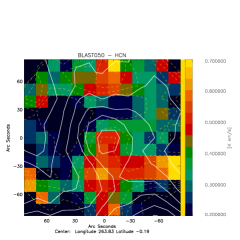
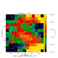
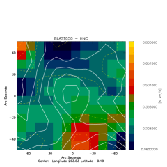
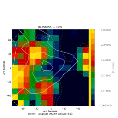
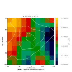
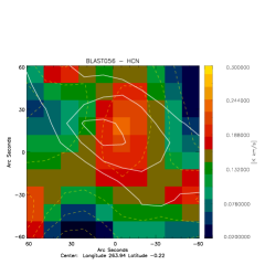
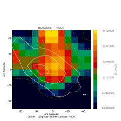
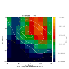
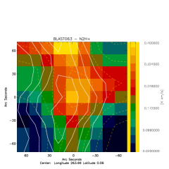
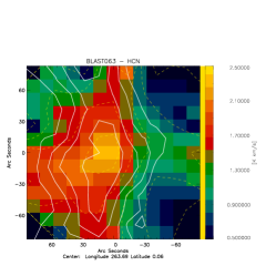
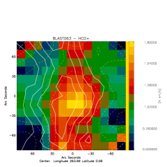
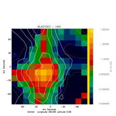
Figure 13: Same as Figure 11 for sources BLAST050, BLAST055, BLAST056 and BLAST063.

Appendix B Molecular line spectra

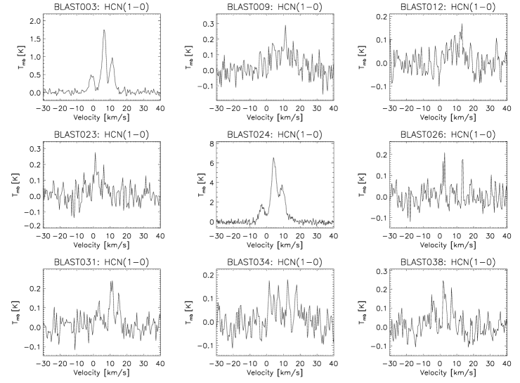
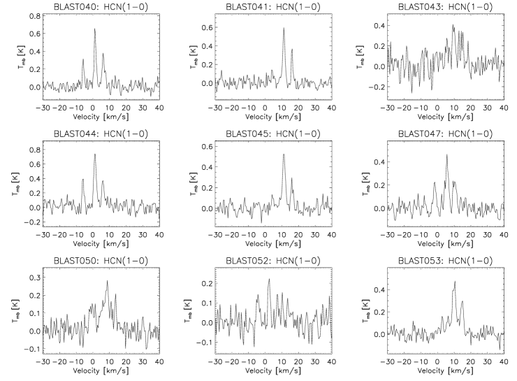
Figure 16: Same as Figure 15 for the HCN$(1-0)$ line

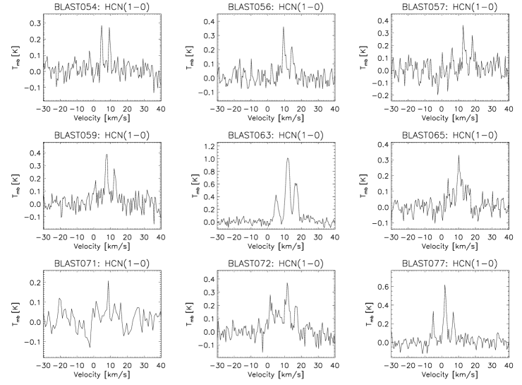
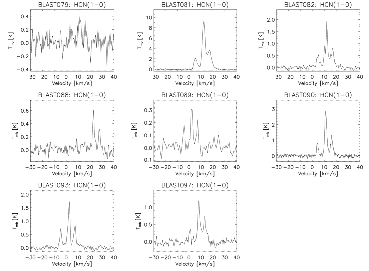
Figure 17: Ctnd. from Figure 16

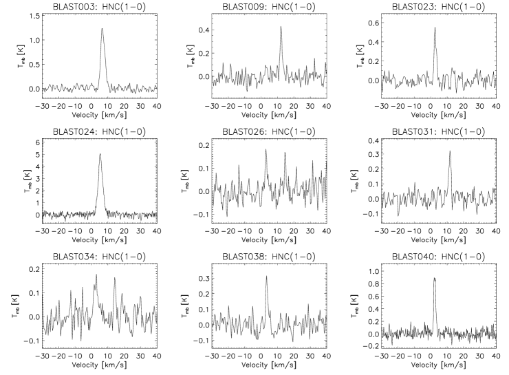
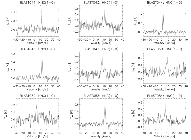
Figure 18: Same as Figure 15 for the HNC$(1-0)$ line

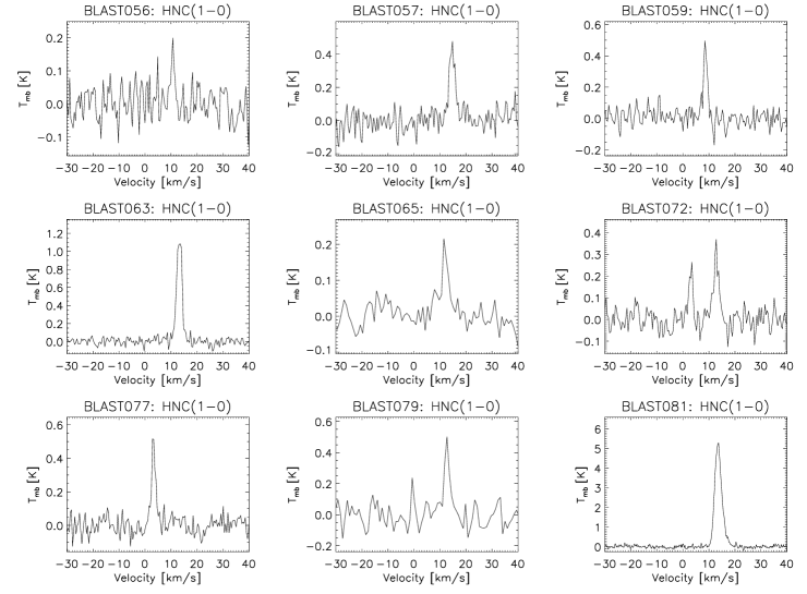
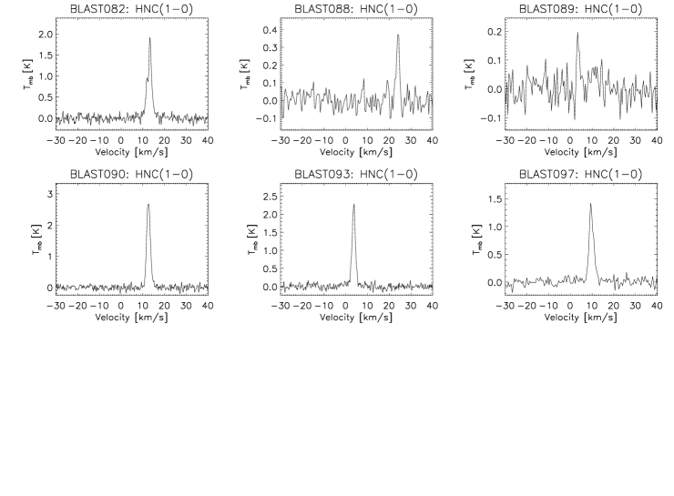
Figure 19: Ctnd. from Figure 18

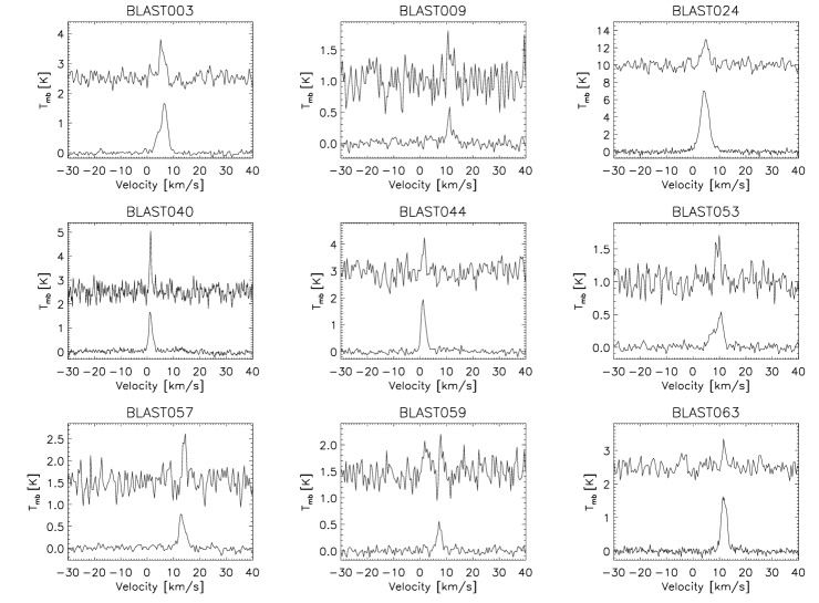
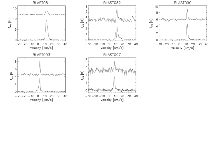
Figure 20: Same as Figure 15 for the HCO${}^{+}(1-0)$ (lower spectra) and H¹³CO${}^{+}(1-0)$ (upper spectra) lines. Only sources where H¹³CO${}^{+}(1-0)$ was detected are shown.

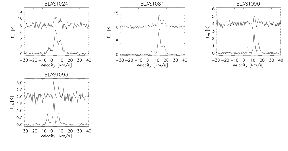
Figure 21: Same as Figure 15 for the H¹³CN$(1-0)$ (upper spectra) lines, shown together with the corresponding HCN$(1-0)$ (lower spectra) lines. Only sources where H¹³CN$(1-0)$ was detected are shown.

Appendix C Molecular lines parameters

Table 12: N₂H⁺ line parameters.

Source #	N2H+
	$T_{A}^{\star}\,\tau$	$V_{lsr}$	FWHM	$\tau$	$T_{ex}$
	[K]	[km s-1]	[km s-1]		[K]
3	0.57	4.3	1.0	0.72	4.5
9	0.35	9.8	0.7	0.10	–
24	2.84	3.2	2.3	0.10	–
40	0.79	0.3	0.7	0.10	–
44	0.79	0.2	0.9	0.25	–
45	0.28	10.4	1.1	0.10	–
63	0.34	11.2	1.6	0.78	3.7
81	3.05	11.6	2.7	0.10	–
82	1.38	10.8	1.6	0.65	7.2
90	1.51	10.4	1.4	0.90	6.3
93	1.40	1.5	1.5	0.72	6.9
97	0.55	7.7	1.6	1.09	3.8

Table 13: HCN and H¹³CN line parameters.

Source #	HCN						H13CN
	$T_{A}^{\star}\,\tau$	$V_{lsr}$	FWHM	$\tau$	$T_{ex}$		$T_{A}^{\star}\,\tau$	$V_{lsr}$	FWHM	$\tau$
	[K]	[km s-1]	[km s-1]		[K]		[K]	[km s-1]	[km s-1]
3	0.83	7.1	2.8	0.12	–		–	–	–	–
24	3.12	5.1	3.6	0.16	–		0.25	2.8	2.9	0.18
26	0.06	3.1	1.7	0.10	–		–	–	–	–
26	0.06	3.1	1.7	0.10	–		–	–	–	–
31	0.22	11.4	2.0	2.06	3.0		–	–	–	–
38	1.17	3.6	1.2	17.03	2.9		–	–	–	–
40	0.43	2.2	1.3	0.83	3.8		–	–	–	–
41	0.29	12.1	1.4	0.10	–		–	–	–	–
43	0.21	9.7	5.2	1.77	3.0		–	–	–	–
44	0.49	2.1	1.6	0.84	4.0		–	–	–	–
45	0.24	12.1	1.9	0.10	–		–	–	–	–
47	0.50	6.4	1.8	3.08	3.1		–	–	–	–
50	0.93	7.7	2.9	13.81	2.9		–	–	–	–
52	0.36	3.3	1.1	4.13	2.9		–	–	–	–
53	0.22	10.7	2.6	0.10	–		–	–	–	–
54	0.42	5.4	0.9	3.21	3.0		–	–	–	–
56	0.16	10.4	1.9	0.10	–		–	–	–	–
57	0.38	14.2	1.5	3.06	3.0		–	–	–	–
59	0.23	8.4	1.9	0.53	3.7		–	–	–	–
63	0.78	12.7	2.4	1.11	4.2		–	–	–	–
77	0.28	2.9	1.8	0.10	–		–	–	–	–
79	0.36	12.1	2.1	2.02	3.1		–	–	–	–
81	4.05	13.2	3.1	0.10	–		0.38	11.3	3.1	0.10
82	0.67	12.8	3.0	0.11	–		–	–	–	–
88	0.27	23.7	1.8	0.10	–		–	–	–	–
89	0.35	3.1	1.5	2.08	3.1		–	–	–	–
90	1.27	12.1	2.1	0.10	–		0.12	10.2	1.6	0.18
93	0.80	3.1	2.2	0.24	–		0.11	1.1	1.5	0.10
97	0.53	9.1	2.7	0.10	–		–	–	–	–

Table 14: HNC line parameters.

Source #	HNC
	$\int{T_{A}^{\star}\,{\rm d}V}$	$V_{lsr}$	FWHM
	[K km s-1]	[km s-1]	[km s-1]
3	1.79	6.9	2.9
9	0.31	12.2	1.5
23	0.42	2.7	1.6
24	7.68	5.5	3.2
26	0.12	3.1	1.4
26	0.08	14.7	0.8
31	0.25	11.7	1.6
34	0.21	2.7	2.9
38	0.21	3.4	1.3
40	0.66	2.4	1.4
41	0.23	12.1	1.1
43	0.42	11.1	1.5
44	0.90	2.4	1.5
45	0.44	12.6	1.7
52	0.20	3.7	1.9
53	0.53	11.3	1.8
54	0.22	5.7	1.7
56	0.14	10.6	1.6
57	0.61	14.7	2.8
59	0.42	8.6	1.8
63	1.38	13.2	2.4
72	0.36	12.8	2.4
77	0.46	3.3	1.8
79	0.55	12.7	2.3
81	8.07	13.6	3.1
82	1.97	13.1	2.5
88	0.30	24.0	1.5
89	0.13	3.6	1.4
90	2.71	12.6	2.0
93	2.01	3.7	1.8
97	1.64	9.7	2.5

Table 15: HCO⁺ and H¹³CO⁺ Line Parameters.

Source #	HCO+							H13CO+
	$T_{A}^{\star}\,\tau$	$V_{lsr}$	FWHM	$\tau$	$T_{ex}$	Line Wings?		$T_{A}^{\star}\,\tau$	$V_{lsr}$	FWHM	$\tau$
	[K]	[km s-1]	[km s-1]		[K]			[K]	[km s-1]	[km s-1]
3	2.66	6.3	3.6	7.97	4.4	NG		0.33	5.6	2.4	0.20
9	0.45	11.1	1.9	12.07	3.3	NG		0.17	11.3	2.8	0.30
23	0.37	1.2	0.9	–	3.7	N		–	–	–	–
24	13.00	4.4	3.8	4.13	10.1	Y		0.99	4.7	2.9	0.10
26	0.31	1.9	2.0	–	3.1	N		–	–	–	–
26	0.20	13.5	1.5	–	3.1	N		–	–	–	–
31	0.60	10.4	1.7	–	3.6	N		–	–	–	–
34	0.50	2.0	2.0	–	3.3	N		–	–	–	–
34	0.24	13.1	1.6	–	3.1	N		–	–	–	–
38	0.36	1.9	1.8	–	3.2	N		–	–	–	–
40	1.30	1.3	1.7	–	4.5	N		0.23	1.3	0.8	–
41	0.62	11.0	1.4	–	3.7	N		–	–	–	–
43	0.63	9.9	1.4	–	3.8	N		–	–	–	–
44	1.85	1.2	2.0	6.65	4.8	N		0.16	1.5	1.1	0.17
45	1.14	11.1	2.1	–	4.0	NG		–	–	–	–
47	0.37	5.4	2.5	–	3.1	N		–	–	–	–
47	0.18	9.2	1.3	–	3.1	N		–	–	–	–
52	0.44	2.3	2.3	–	3.2	N		–	–	–	–
54	0.24	4.7	1.9	–	3.1	N		–	–	–	–
56	0.35	9.4	2.0	–	3.2	N		–	–	–	–
57	1.04	13.2	2.9	–	3.6	N		0.21	14.1	1.5	–
59	0.51	7.3	2.1	–	3.3	N		0.08	7.8	0.9	–
63	2.04	11.7	2.5	4.99	4.6	Y		0.13	11.8	1.4	0.12
71	0.17	7.5	2.1	–	3.0	N		–	–	–	–
72	0.86	1.9	2.1	–	3.7	N		–	–	–	–
72	0.58	11.6	2.9	–	3.2	N		–	–	–	–
77	1.00	1.8	2.1	–	3.9	N		–	–	–	–
79	0.87	11.0	3.8	–	3.3	N		–	–	–	–
81	16.33	12.4	3.6	2.07	13.7	Y		0.95	12.5	3.6	0.05
82	0.66	10.0	1.1	–	4.1	Y		0.44	11.9	1.8	–
82	2.52	12.6	2.5	11.49	5.0	Y		0.44	11.9	1.8	0.29
89	0.57	2.3	2.4	–	3.3	N		–	–	–	–
90	5.37	11.4	2.3	7.57	7.8	Y		0.65	11.5	1.6	0.19
93	3.52	2.1	2.3	14.82	6.1	Y		0.73	2.5	1.5	0.37
97	1.81	8.1	2.2	6.64	4.6	Y		0.28	8.7	2.2	0.17

References

- Aikawa et al. (2008) Aikawa, Y., Wakelam, V., Garrod, R. T., & Herbst, E. 2008, ApJ, 674, 984
- Bachiller et al. (1987) Bachiller, R., Guilloteau, S., & Kahane, C. 1987, A&A, 173, 324
- Benson et al. (1998) Benson, P. J., Caselli, P., & Myers, P. C. 1998, ApJ, 506, 743
- Blake et al. (1995) Blake, G. A., Sandell, G., van Dishoeck, E. F., et al. 1995, ApJ, 441, 689
- Carey et al. (2005) Carey, S. J., Noriega-Crespo, A., Price, S. D., et al. 2005, in Bulletin of the American Astronomical Society, 1252
- Caselli et al. (2002) Caselli, P., Benson, P. J., Myers, P. C., & Tafalla, M. 2002, ApJ, 572, 238
- Elia et al. (2007) Elia, D., Massi, F., Strafella, F., et al. 2007, ApJ, 655, 316
- Evans (1999) Evans, II, N. J. 1999, ARA&A, 37, 311
- Friesen et al. (2010) Friesen, R. K., Di Francesco, J., Shimajiri, Y., & Takakuwa, S. 2010, ApJ, 708, 1002
- Fuente et al. (2005) Fuente, A., Rizzo, J. R., Caselli, P., Bachiller, R., & Henkel, C. 2005, A&A, 433, 535
- Giannini et al. (2007) Giannini, T., Lorenzetti, D., De Luca, M., et al. 2007, ApJ, 671, 470
- Godard et al. (2010) Godard, B., Falgarone, E., Gerin, M., Hily-Blant, P., & de Luca, M. 2010, A&A, 520, A20
- Goodman et al. (1993) Goodman, A. A., Benson, P. J., Fuller, G. A., & Myers, P. C. 1993, ApJ, 406, 528
- Hirota et al. (1998) Hirota, T., Yamamoto, S., Mikami, H., & Ohishi, M. 1998, ApJ, 503, 717
- Kruegel & Walmsley (1984) Kruegel, E. & Walmsley, C. M. 1984, A&A, 130, 5
- Lada et al. (2008) Lada, C. J., Muench, A. A., Rathborne, J., Alves, J. F., & Lombardi, M. 2008, ApJ, 672, 410
- Ladd et al. (2005) Ladd, N., Purcell, C., Wong, T., & Robertson, S. 2005, PASA, 22, 62
- Lee et al. (2004) Lee, J.-E., Bergin, E. A., & Evans, II, N. J. 2004, ApJ, 617, 360
- Liseau et al. (1992) Liseau, R., Lorenzetti, D., Nisini, B., Spinoglio, L., & Moneti, A. 1992, A&A, 265, 577
- MacLaren et al. (1988) MacLaren, I., Richardson, K. M., & Wolfendale, A. W. 1988, ApJ, 333, 821
- Mardones et al. (1997) Mardones, D., Myers, P. C., Tafalla, M., et al. 1997, ApJ, 489, 719
- Massi et al. (2007) Massi, F., De Luca, M., Elia, D., et al. 2007, A&A, 466, 1013
- Molinari et al. (2010) Molinari, S., Swinyard, B., Bally, J., et al. 2010, A&A, 518, L100
- Motte et al. (1998) Motte, F., André, P., & Neri, R. 1998, A&A, 336, 150
- Murphy & May (1991) Murphy, D. C. & May, J. 1991, A&A, 247, 202
- Netterfield et al. (2009) Netterfield, C. B., Ade, P. A. R., Bock, J. J., et al. 2009, ApJ, 707, 1824
- Nikolić et al. (2003) Nikolić, S., Johansson, L. E. B., & Harju, J. 2003, A&A, 409, 941
- Olmi et al. (2009) Olmi, L., Ade, P. A. R., Anglés-Alcázar, D., et al. 2009, ApJ, 707, 1836
- Olmi et al. (2010) Olmi, L., Araya, E. D., Chapin, E. L., et al. 2010, ApJ, 715, 1132
- Olmi & Testi (2002) Olmi, L. & Testi, L. 2002, A&A, 392, 1053
- Pascale et al. (2008) Pascale, E., Ade, P. A. R., Bock, J. J., et al. 2008, ApJ, 681, 400
- Patanchon et al. (2008) Patanchon, G. et al. 2008, ApJ, 681, 708
- Pirogov & Zinchenko (1993) Pirogov, L. E. & Zinchenko, I. I. 1993, Astronomy Reports, 37, 484
- Saito et al. (2008) Saito, H., Saito, M., Yonekura, Y., & Nakamura, F. 2008, ApJS, 178, 302
- Tafalla et al. (2004) Tafalla, M., Myers, P. C., Caselli, P., & Walmsley, C. M. 2004, A&A, 416, 191
- Tafalla et al. (2002) Tafalla, M., Myers, P. C., Caselli, P., Walmsley, C. M., & Comito, C. 2002, ApJ, 569, 815
- Truch et al. (2008) Truch, M. D. P. et al. 2008, ApJ, 681, 415
- Ungerechts et al. (1986) Ungerechts, H., Winnewisser, G., & Walmsley, C. M. 1986, A&A, 157, 207
- van der Tak et al. (2007) van der Tak, F. F. S., Black, J. H., Schöier, F. L., Jansen, D. J., & van Dishoeck, E. F. 2007, A&A, 468, 627
- Womack et al. (1992) Womack, M., Ziurys, L. M., & Wyckoff, S. 1992, ApJ, 387, 417
- Zinchenko et al. (2009) Zinchenko, I., Caselli, P., & Pirogov, L. 2009, MNRAS, 395, 2234