Optimal Threshold Control by the Robots of Web Search Engines with Obsolescence of Documents

Abstract

A typical Web Search Engine consists of three principal parts: crawling engine, indexing engine, and searching engine. The present work aims to optimize the performance of the crawling engine. The crawling engine finds new Web pages and updates Web pages existing in the database of the Web Search Engine. The crawling engine has several robots collecting information from the Internet. We first calculate various performance measures of the system (e.g., probability of arbitrary page loss due to the buffer overflow, probability of starvation of the system, the average time waiting in the buffer). Intuitively, we would like to avoid system starvation and at the same time to minimize the information loss. We formulate the problem as a multi-criteria optimization problem and attributing a weight to each criterion we solve it in the class of threshold policies. We consider a very general Web page arrival process modeled by Batch Marked Markov Arrival Process and a very general service time modeled by Phase-type distribution. The model has been applied to the performance evaluation and optimization of the crawler designed by INRIA Maestro team in the framework of the RIAM INRIA-Canon research project.

1 Introduction

The problem of control by the robots (crawlers) that traverse the Web and bring Web pages to the indexing engine that updates the data base of a Web Search Engine is formulated and analyzed in [13]. This problem is formulated in [13] as the controlled queueing system. The system has a single server with the exponential service time distribution, finite buffer of capacity $K-1,\;K\geq 2.$ There are $N$ available robots and each of these robots, when activated, brings pages to the server in a Poisson stream at fixed rate. These $N$ stationary Poisson processes are mutually independent and independent of service times.

The number of active robots may be modified at any arrival or departure epoch. When an arrival occurs, the incoming robot is de-activated at once; the controller may then decide to keep it idle or to activate it. When a departure occurs the controller may either decide to activate one additional robot, if one is available, or to do nothing (i.e. the number of active robots is left unchanged).

In [13], the problem of finding a policy that minimizes a weighted sum of the loss rate and starvation probability (probability of the empty system) is considered. It is solved by means of the tools of the Markov Decision Problems theory.

As the possible generalizations of the model, which are certainly worthwhile analyzing, the following ones are mentioned in [13]:

• More general input processes, e.g., a $MMPP$ (Markov Modulated Poisson Process) should be considered so as to reflect more accurately “traveling times” of robots in the network;

• Because of the obsolescence of stored documents issue, the waiting time should be bounded, even if the buffer size is effectively infinite;

• Other cost functions could be investigated, for instance, cost functions including response times.

In this paper, we made all the mentioned and some further generalizations.

We assume that, under the fixed number of currently active robots, the arrival process is of the $BMAP$ type. The $BMAP$ is a more general process comparing to the $MMPP$ and allows delivering of a batch of Web pages to be indexed while the $MMPP$ assumes that the pages are delivered one-by-one. It is very typical for a computer system to operate in batch mode.

We assume that the service time distribution is of the $PH$ (Phase) type which is much more general comparing to the exponential distribution assumed in [13]. The class of phase type distributions is dense in the field of all positive-valued distributions and practically we can deal with any real distribution [2].

Since web pages can become obsolete, we bound the waiting time stochastically. Waiting time of each web page in a buffer is restricted by a random variable having $PH$ distribution identical and mutually independent for all Web pages. The phase type distribution has been used to model obsolescence times for instance in [15].

We suppose that the cost function can have a more general form than in [13] and include the obsolescence probability and response time.

In the next section we formulate the model and optimization problem. Section 3 contains the steady-state analysis of the multi-dimensional Markov chain which defines dynamics of the system under the fixed values of the parameters defining the strategy of control. In Section 4, main performance measures of the system are computed. In Section 5, the conditional sojourn time distributions are calculated. In Section 6, the case of ordinary arrivals is touched in brief. In Section 7, the theoretical results are illustrated by numerical examples. In particular, the mathematical model is applied to the performance evaluation and optimization of the robot designed by INRIA Maestro team in the framework of the RIAM INRIA-Canon research project. Section 8 concludes the paper.

2 Mathematical Model

We consider a single server system with the finite buffer of capacity $K-1,\;K\geq 2.$ So, the total number of Web pages which can stay in the system is restricted by the number $K.$ Web pages are served by a server in order of their arrivals.

Service times of Web pages are independent identically distributed random variables having $PH$ distribution with irreducible representation $({\boldsymbol{\beta}},S).$ It means the following. Service of a Web page is defined as a time until the continuous-time Markov chain $m_{t},\;t\geq 0,$ having the states $(1,\dots,M)$ as the transient and state $0$ as absorbing one reaches the absorbing state. An initial state of the chain is selected in a random way, according to the probability distribution defined by the row-vector $({\boldsymbol{\beta}},0)$, where ${\boldsymbol{\beta}}$ is the stochastic row vector of dimension $M$. Transitions of the Markov chain $m_{t},\;t\geq 0$, are described by the generator $\left(\begin{array}[]{cc}S&S_{0}\cr 0&0\end{array}\right)$ where the matrix $S$ is a sub-generator and the column vector $S_{0}$ is defined by $S_{0}=-S{\bf e}_{M}\;$ and has all non-negative and at least one positive components, ${\bf e}_{M}$ is the column vector of dimension $M$ consisting of all 1’s. The average service time $b_{1}$ is given by $b_{1}={\boldsymbol{\beta}}(-S)^{-1}{\bf e}_{M}.$ For more details about the $PH$ type distribution, its properties, special cases and applications see [11, 12].

Web pages can be delivered into the system by $N$ available robots. The number of active robots varies in the set $\{1,\dots,N\}.$ We assume that the process of Web pages delivering under $l,\;l=\overline{1,N},$ active robots is described as follows. Let $\nu_{t},\;t\geq 0,$ be an irreducible continuous time Markov chain having finite state space $\{0,1,\dots,W\}$. Sojourn time of the chain $\nu_{t},\,t\ \geq 0$, in the state $\nu$ has exponential distribution with a parameter $\lambda^{(l)}_{\nu}$. After this time expires, with probability $p^{(l)}_{0}(\nu,\nu^{\prime})$ the chain jumps into the state $\nu^{\prime}$ without generation of Web pages and with probability $p^{(l)}_{k}(\nu,\nu^{\prime})$ the chain jumps into the state $\nu^{\prime}$ and a batch consisting of $k$ Web pages is generated, $k\geq 1$. The introduced probabilities satisfy conditions:

$$p^{(l)}_{0}(\nu,\nu)=0,\,\;\sum\limits_{k=1}^{\infty}\sum\limits_{\nu^{\prime}=0}^{W}p_{k}^{(l)}(\nu,\nu^{\prime})+\sum\limits_{\nu^{\prime}=0}^{W}p_{0}^{(l)}(\nu,\nu^{\prime})=1,\;\;\nu=\overline{0,W},\;l=\overline{1,N}.$$

The parameters defining this flow are kept in the square matrices ${\mathcal{D}}_{k}^{(l)},\,k\geq 0,\;l=\overline{1,N},$ of size $\bar{W}=W+1$ defined by their entries:

$$({\mathcal{D}}^{(l)}_{0})_{\nu,\nu}=-\lambda^{(l)}_{\nu},\,({\mathcal{D}}^{(l)}_{0})_{\nu,\nu^{\prime}}=\lambda^{(l)}_{\nu}p_{0}(\nu,\nu^{\prime}),$$

$$({\mathcal{D}}_{k}^{(l)})_{\nu,\nu^{\prime}}=\lambda^{(l)}_{\nu}p_{k}^{(l)}(\nu,\nu^{\prime}),\,\nu,\nu^{\prime}=\overline{0,W},\,k\geq 1,\,l=\overline{1,N}.$$

Denote

$${\mathcal{D}}^{(l)}(z)=\sum\limits_{k=0}^{\infty}{\mathcal{D}}^{(l)}_{k}z^{k},\;|z|\leq 1.$$

The matrix ${\mathcal{D}}^{(l)}(1)$ is the infinitesimal generator of the process ${\nu_{t}},t\geq 0,$ under the fixed number $l$ of active robots. The stationary distribution vector ${\boldsymbol{\theta}}^{(l)}$ of this process satisfies the equations ${\boldsymbol{\theta}}^{(l)}{\mathcal{D}}^{(l)}(1)={\boldsymbol{0}},{\boldsymbol{\theta}}^{(l)}{\bf e}=1.$ Here and in the sequel, ${\boldsymbol{0}}$ is the zero row vector. The average intensity $\lambda^{(l)}$ (fundamental rate) of the $BMAP$ under the fixed number $l$ of active robots is defined by

$$\lambda^{(l)}={\boldsymbol{\theta}}^{(l)}\frac{d{\mathcal{D}}^{(l)}(z)}{dz}|_{z=1}{\bf e},$$

and the intensity $\lambda^{(l)}_{g}$ of group arrivals is defined by

$$\lambda^{(l)}_{g}={\boldsymbol{\theta}}^{(l)}(-{\mathcal{D}}^{(l)}_{0}){\bf e}.$$

The variance $v^{(l)}$ of intervals between group arrivals is calculated as

$$v^{(l)}=2({\lambda^{(l)}_{g}})^{-1}{\boldsymbol{\theta}}^{(l)}(-{\mathcal{D}}^{(l)}_{0})^{-1}{\bf e}-({\lambda^{(l)}_{g}})^{-2},$$

while the correlation coefficient $c^{(l)}_{cor}$ of intervals between successive group arrivals is given by

$$c^{(l)}_{cor}=\frac{1}{v(\lambda^{(l)}_{g})^{2}}\biggl{(}\lambda^{(l)}_{g}{\boldsymbol{\theta}}^{(l)}(-{\mathcal{D}}^{(l)}_{0})^{-1}({\mathcal{D}}(1)^{(l)}-{\mathcal{D}}^{(l)}_{0})(-{\mathcal{D}}^{(l)}_{0})^{-1}{\bf e}-1\biggr{)}.$$

The introduced representation of the arrival process via the matrices ${\mathcal{D}}_{k}^{(l)},\,k\geq 0,\;l=\overline{1,N},$ unifies several possible interpretations of the process of Web pages delivered by the fixed number of active robots:

• The processes of Web pages delivering by all robots are independent $BMAP$ processes. Let the process of Web pages delivering by the $l$th robot be the $BMAP$ which is governed by the continuous time Markov chain $\nu_{t}^{(l)},\;t\geq 0,$ having finite state space $\{0,1,\dots,W_{l}\}$ and defined by the matrices $D_{k}^{(l)},\,k\geq 0,\;$ of size $\bar{W}_{l}=W_{l}+1.$ See [10] for more details about the $BMAP$, its properties and special cases. We denote $D^{(l)}(z)=\sum\limits_{k=0}^{\infty}D_{k}^{(l)}z^{k},\;|z|\leq 1.$

  Let us assume that the robots are arranged in such a way that the first robot is always active, then, when a queue decreases, the second robot can be activated, etc, the $N$th robot is the most rare activated.

  The matrices ${\mathcal{D}}_{k}^{(l)},\,k\geq 0,\;l=\overline{1,N},$ of size $\bar{W}=\prod\limits_{k=1}^{N}\bar{W}_{k}$ defined by formulae (1) are expressed via the matrices $D_{k}^{(l)},\;k\geq 0,\;$ of size $\bar{W}_{l},\;l=\overline{1,N},$ describing the $BMAP$s in the following way:

  $${\mathcal{D}}^{(l)}_{0}=D_{0}^{(1)}\oplus D_{0}^{(2)}\oplus\dots\oplus D_{0}^{(l)}\otimes D^{(l+1)}(1)\otimes\dots\otimes D^{(N)}(1),$$

  $${\mathcal{D}}^{(l)}_{k}=D_{k}^{(1)}\oplus D_{k}^{(2)}\oplus\dots\oplus D_{k}^{(l)}\otimes I_{\bar{W}_{l+1}}\otimes\dots\otimes I_{\bar{W}_{N}},\;\;k\geq 1.$$

  Here $\otimes$ and $\oplus$ denote Kronecker product and sum of matrices correspondingly (see, e.g., [7]), $I_{L}$ denotes identity matrix of size $L.$ If the size of the matrix is clear from context the suffix can be omitted. $I_{0}\stackrel{{\scriptstyle def}}{{=}}1.$

• The common process of Web pages delivered by all robots together is the $BMAP$ process directed by the continuous time Markov chain $\nu_{t},\;t\geq 0,$ having finite state space $\{0,1,\dots,W\}$ and defined by the matrices $D_{k},\,k\geq 0,\;$ of size $\bar{W}.$ Some set of thinning probabilities $q_{1},\dots,q_{N},\;$ $0<q_{1}<\dots<q_{N}=1,\;$ is fixed. When $l$ robots are active, procedure of thinning the $BMAP$ process with the thinning probability $q_{l}$ is applied. It means that an arbitrary arriving batch is accepted with probability $q_{l}$ and is rejected with the complimentary probability $1-q_{l}.$ We denote $D(z)=\sum\limits_{k=0}^{\infty}D_{k}z^{k},\;|z|\leq 1.$

  The matrices ${\mathcal{D}}_{k}^{(l)},\,k\geq 0,\;l=\overline{1,N},$ defined by formulae (1) are expressed via the matrices $D_{k},\,k\geq 0,\;$ describing the common $BMAP$ and via the thinning probability $q_{l}$ in the following way:

  $${\mathcal{D}}^{(l)}_{0}=D_{0}q_{l}+D(1)(1-q_{l}),\;\;{\mathcal{D}}^{(l)}_{k}=D_{k}q_{l},\;k\geq 1.$$

• Let the process of Web pages delivering by robots is described by a $BMMAP.$ The $BMMAP$ is directed by continuous time Markov chain $\nu_{t},\;t\geq 0,$ having finite state space $\{0,1,\dots,W\}$. Sojourn time of the chain $\nu_{t},\,t\ \geq 0$, in the state $\nu$ has exponential distribution with a parameter $\lambda_{\nu}$. After this time expires, with probability $p_{0}(\nu,\nu^{\prime})$ the chain jumps into the state $\nu^{\prime}$ without generation of Web pages and with probability $p^{(l)}_{k}(\nu,\nu^{\prime})$ the chain jumps into the state $\nu^{\prime}$ and a batch consisting of $k,\;$$k\geq 1$ Web pages are delivered by the $l$th robot. The introduced probabilities satisfy conditions:

  $$p_{0}(\nu,\nu)=0,\,\,\sum\limits_{l=1}^{N}\sum\limits_{k=1}^{\infty}\sum\limits_{\nu^{\prime}=0}^{W}p_{k}^{(l)}(\nu,\nu^{\prime})+\sum\limits_{\nu^{\prime}=0}^{W}p_{0}(\nu,\nu^{\prime})=1,\;\;\nu=\overline{0,W}.$$

  The matrices ${\mathcal{D}}_{k}^{(l)},\,k\geq 0,\;l=\overline{1,N},$ defined by formulae (1) are expressed via the matrices $D_{0},\;D^{(l)}_{k},\,k\geq 1,\;l=\overline{1,N},$ formed by the probabilities $p_{0}(\nu,\nu)$ and $p_{k}^{(l)}(\nu,\nu^{\prime})$ in the following way:

  $${\mathcal{D}}^{(l)}_{0}=D_{0}+\sum\limits_{j=1}^{\infty}\sum\limits_{m=l+1}^{N}D^{(m)}_{j},\;{\mathcal{D}}^{(l)}_{k}=\sum\limits_{m=1}^{l}D^{(m)}_{k},\;k\geq 1.$$

• The process of Web pages delivery by all robots is the $BMAP$ process directed by the continuous time Markov chain $\nu_{t},\;t\geq 0,$ having finite state space $\{0,1,\dots,W\}$ and defined by the transition intensity matrices ${\mathcal{D}}_{k}^{(l)},\,k\geq 0,\;l=\overline{1,N},$ depending on the number of active robots.

Interpretation 3 seems be the most attractive because it assumes that the work of the robots can be dependent, which is quite realistic. Because the total amount of Web servers from which new pages should be brought is more or less constant, reduction of the number of active robots causes the increase of field in Internet, which is scrawled by each robot, and corresponding change of travel time. So, the $BMMAP$ looks to be the most realistic model of Web pages delivery.

If a batch of delivered Web pages meets free server one Web page starts the service immediately while the rest moves to the buffer. If the server is busy at an arrival epoch, all Web pages of the batch are placed into the buffer if there is enough free space in the buffer. If the number of free places in the buffer is less than the number of Web pages in the batch, the corresponding number of Web pages is lost. It means that we consider so called partial admission strategy. The alternative strategies of complete rejection or complete admission can be investigated in analogous way.

For each Web page placed into the buffer, the waiting time is restricted by the random variable (so called obsolescence time) having $PH$ distribution with irreducible representation $({\boldsymbol{\gamma}},\Gamma).$ It means the following. Available waiting time of the $i$th Web page in the buffer is defined as a time until the continuous-time Markov chain $r_{t}^{(i)},\;t\geq 0,$ having the states $(1,\dots,R)$ as the transient and state $0$ as absorbing one, reaches the absorbing state. Transition of this process into the absorbing state means that this Web page gets out of date (obsolescence or dashout occurs). An initial state of the chain is selected in a random way, according to the probability distribution defined by the row-vector $({\boldsymbol{\gamma}},0)$, where ${\boldsymbol{\gamma}}$ is the stochastic row vector of dimension $R$. Transitions of the Markov chain $r_{t}^{(i)},\;t\geq 0$, are described by the generator $\left(\begin{array}[]{cc}\Gamma&\Gamma_{0}\cr 0&0\end{array}\right)$ where the matrix $\Gamma$ is sub-generator and the column vector $\Gamma_{0}$ is defined by $\Gamma_{0}=-\Gamma{\bf e}.$ The average time until obsolescence $g_{1}$ is given by $g_{1}={\boldsymbol{\gamma}}(-\Gamma)^{-1}{\bf e}.$

If the obsolescence time expires before a Web page is picked-up from the buffer to the server, it is assumed that this Web page immediately leaves the buffer and is lost. The obsolescence times of different Web pages are independent of each other and identically distributed. It is worth to note that the analysis presented below could be drastically simplified if we suggest that the obsolescence time is exponentially distributed. However, this suggestion rarely holds true in the real world systems because this suggestion means that, with high probability, information obsoletes very quickly.

Reasonable class of strategies of control by robots is the class of the threshold strategies defined as follows. Integers $j_{1},\dots,j_{N-1}$ are fixed such as $-1=j_{0}<j_{1}<\dots<j_{N-1}<j_{N}=K.$ If the number $i$ of Web pages in the system satisfies inequality $j_{r-1}+1\leq i\leq j_{r},$ then $N-r+1$ robots are active and $r-1$ robots are de-activated, $r=\overline{1,N}.$

Note that the described threshold strategies are popular in literature in controlled queues, see, e.g., [1, 3, 5, 6, 14]. For some systems, it is proven that the optimal strategy in the class of all Markovian strategies belongs to the class of threshold strategies. For some other systems such a result is not proven, but the optimal strategy is sought in the class of threshold strategies. Advantage of such strategies is their intuitive justification and relative simplicity of implementation in real-life systems. Numerical examples presented in the paper [13] for a partial case of our model confirm that the threshold strategies are optimal in the class of all Markovian strategies, although authors cannot prove this fact. Our system is much more complicated and we also cannot prove optimality of the optimal threshold strategy in wider classes of strategies. We just try to find an optimal threshold strategy and believe that it is optimal or sub-optimal in wider classes as well.

We also mention that the description of the given above threshold strategy suits only for the case when $N\leq K.$ While the numerical examples presented in [13] address, e.g., the case $N=16$ and $K=5$. However, if we look at the optimal strategy given by Figure 2 in [13], we see that the optimal number of the active robots varies between 4 and 14 with 4 switching points where two or three robots are activated or de-activated. Because, in contrast to [13], we do not assume that each active robot generates a stationary Poisson process of arrivals at a fixed rate but we assume that each robot generates a batch Markovian arrival process, we see that our strategy suits for the case $N>K$ as well. We could achieve this formally by allowing non-strict inequalities: $-1=j_{0}\leq j_{1}\leq\dots\leq j_{N-1}\leq j_{N}=K$ in fixing the thresholds. So, speaking below about a robot we may think about a virtual robot as a group of several available real robots which are activated and de-activated simultaneously.

We will solve the problem of choosing the optimal threshold strategy. The cost function is assumed to be of the following form:

$$J=\lambda(c_{loss}P_{loss}+c_{obs}P_{obs})+a\bar{V}^{(1)}+c_{rob}N_{act}+c_{star}P_{star}$$

where $\lambda$ is the mean number of pages delivered into the system by robots during a unit of time (fundamental rate of the arrival process), $P_{loss}$ is probability of arbitrary page loss due to the buffer overflow, $P_{obs}$ is probability of arbitrary page obsolescence during waiting in a queue, $P_{star}$ is probability of starvation of the system, $\bar{V}^{(1)}$ is the response time (average sojourn time of Web pages which are not lost or deleted due to obsolescence), $N_{act}$ is the average number of active robots, $c_{loss},c_{obs},a,c_{rob},c_{star}$ are the corresponding non-negative cost coefficients. The values of the cost coefficients can be set up by experts in the domain. Alternatively, the cost coefficients can be viewed as Lagrange multipliers in the constrained problem and can be found from the dual problem formulation.

It is clear that if the average number of active robots is increasing then the three first summands in (2) are increasing while the last summand, charge for starvation of the system, is decreasing. The last charge is important because starvation means that the indexing machine is idle and so freshness of the data base suffers.

The problem of minimization of the cost criterion (2) is not trivial. To solve this problem, we will use so called direct approach. To this end, we will calculate the stationary distribution of the system state under an arbitrary fixed set of thresholds $(j_{1},\dots,j_{N-1}).$ It will allow us to calculate the main performance measures of the system and the value $J$ of the cost criterion as a function $J(j_{1},\dots,j_{N-1}).$ Problem of finding the optimal set $(j^{*}_{1},\dots,j^{*}_{N-1})$ is then easy solved on computer, e.g., by enumeration.

3 Stationary distribution of the number of Web pages in the system

Let some set of thresholds $(j_{1},\dots,j_{N-1})$ be fixed. We are interested in the stationary distribution of the process $i_{t},\;t\geq 0,$ where $i_{t}$ is the number of Web pages in the system at the epoch $t,\;$$i_{t}=\overline{0,K}.$ This process is non-Markovian. To investigate this process, we will consider the following multi-dimensional continuous time Markov chain

$$\xi_{t}=\{i_{t},\nu_{t},m_{t},r_{t}^{(1)},\dots,r_{t}^{(i_{t}-1)}\},\;t\geq 0,$$

where $\nu_{t}$ is the state of the directing process of arrival process at epoch $t,\;$ $\nu_{t}=\overline{0,W};$ $m_{t}$ is the state of the process which directs a service at epoch $t,\;$ $m_{t}=\overline{1,M};$ $r_{t}^{(i)}$ is the state of the process, which directs a obsolescence of the $i$th Web page in a queue at epoch $t,\;$ $r_{t}^{(i)}=\overline{1,R},\;i=\overline{0,K-1}.$

We assume that the Web pages in the buffer are numerated in order of their arrival into the system. If a batch of Web pages arrives to the system, the accepted Web pages are numerated in a uniform random manner. When a Web page is picked up to the service or is deleted from the queue because its admissible waiting time expires, the rest of Web pages is immediately enumerated correspondingly.

Denote

$$p(0,\nu)=\lim\limits_{t\to\infty}P\{i_{t}=0,\nu_{t}=\nu\},$$

$$p(1,\nu,m)=\lim\limits_{t\to\infty}P\{i_{t}=1,\nu_{t}=\nu,m_{t}=m\},$$

$$p(i,\nu,m,r_{1},\ldots,r_{i-1})=$$

$$\lim\limits_{t\to\infty}P\{i_{t}=i,\nu_{t}=\nu,m_{t}=m,r_{t}^{(1)}=r_{1},\ldots,r_{t}^{(i-1)}=r_{i-1}\},\;\;i\geq 2.$$

Because the state space of the the Markov chain $\xi_{t},t\geq 0,$ is finite and due to assumption about irreducibility of the processes defining arrival, service and obsolescence processes, limits (3) exist.

Enumerate the states of the Markov chain $\xi_{t},t\geq 0,$ in the lexicographic order and form the probability row vectors ${\bf p}_{i},i=\overline{0,K},$ of probabilities corresponding to the state $i$ of the first component of the process $\xi_{t},t\geq 0$. Denote also ${\bf p}=({\bf p}_{0},\dots,{\bf p}_{K})$.

Let $Q$ be the infinitesimal generator of the Markov chain $\xi_{t},t\geq 0,$ and $Q_{i,i^{\prime}}$ be the block of the generator $Q$ consisting of enumerated in lexicographic order intensities of transition of the Markov chain $\xi_{t},t\geq 0,$ from the states with the value $i$ of the component $i_{t}$ to the states with the value $i^{\prime}$ of this component, $i,i^{\prime}\geq 0.$ Dimension of the block $Q_{i,i^{\prime}}$ is defined by $(\bar{W}M^{a_{i}}R^{b_{i}})\times(\bar{W}M^{a_{i^{\prime}}}R^{b_{i^{\prime}}})$ where $a_{l}=\min\{l,1\},\;$$b_{l}=\max\{(l-1),0\},\;l=\overline{0,K}.$

Lemma.  Non-zero blocks $Q_{i,i^{\prime}}$ of the infinitesimal generator $Q$ of the Markov chain $\xi_{t},t\geq 0,$ are defined by

$$Q_{0,j}=\left\{\begin{array}[]{lr}{\mathcal{D}}^{(N)}_{0},\;\;j=0,\cr{\mathcal{D}}^{(N)}_{j}\otimes{\boldsymbol{\beta}}\otimes{\boldsymbol{\gamma}}^{\otimes(j-1)},\;\;j=\overline{1,K-1},\cr({\mathcal{D}}^{(N)}(1)-\sum\limits_{r=0}^{K-1}{\mathcal{D}}^{(N)}_{r})\otimes{\boldsymbol{\beta}}\otimes{\boldsymbol{\gamma}}^{\otimes(K-1)},\;\;j=K,\cr\end{array}\right.$$

$$Q_{i,i-1}=\left\{\begin{array}[]{lr}I_{\bar{W}}\otimes S_{0},\;\;i=1,\cr I_{\bar{W}}\otimes{\mathcal{B}}_{i-1},\;i>1,\cr\end{array}\right.$$

$$Q_{i,i}=\left\{\begin{array}[]{lr}{\mathcal{D}}^{(\chi(i))}_{0}\oplus{\mathcal{A}}_{i-1},\;\;i=\overline{1,K-1},\cr{\mathcal{D}}^{(\chi(i))}(1)\oplus{\mathcal{A}}_{i-1},\;\;i=K,\cr\end{array}\right.$$

$$Q_{i,i+l}=\left\{\begin{array}[]{lr}{\mathcal{D}}^{(\chi(i))}_{l}\otimes I_{MR^{i-1}}\otimes{\boldsymbol{\gamma}}^{\otimes l},\;\;l=\overline{1,K-i-1},\;i<K-1,\cr({\mathcal{D}}^{(\chi(i))}(1)-\sum\limits_{r=0}^{K-i-1}{\mathcal{D}}^{(\chi(i))}_{r})\otimes I_{MR^{i-1}}\otimes{\boldsymbol{\gamma}}^{\otimes l},\;\;l=K-i,\;\;i<K,\cr\end{array}\right.$$

$$i>0.$$

Here

$${\mathcal{B}}_{i}=S_{0}{\boldsymbol{\beta}}\otimes{\bf e}_{R}\otimes I_{R^{i-1}}+I_{M}\otimes\Gamma_{0}^{\oplus i},\;{\mathcal{A}}_{i}=S\oplus\Gamma^{\oplus i},\;i=\overline{0,K-1},$$

$${\boldsymbol{\gamma}}^{\otimes l}\stackrel{{\scriptstyle def}}{{=}}\underbrace{{\boldsymbol{\gamma}}\otimes\ldots\otimes{\boldsymbol{\gamma}}}_{l},\;\Gamma^{\oplus l}\stackrel{{\scriptstyle def}}{{=}}\underbrace{\Gamma\oplus\ldots\oplus\Gamma}_{l},\;\Gamma_{0}^{\oplus l}\stackrel{{\scriptstyle def}}{{=}}\underbrace{\Gamma_{0}\oplus\ldots\oplus\Gamma_{0}}_{l},\quad l\geq 1,$$

and the value $\chi(i),$ which corresponds to the number of active robots when $i$ Web pages stay in the system, is calculated by $\chi(i)=N-\psi(i)$ where the value $\psi(i),\;\psi(i)=\overline{0,N-1},$ is defined by relations

$$j_{\psi(i)}+1\leq i\leq j_{\psi(i)+1},\;i=\overline{0,K}.$$

Proof of the lemma is implemented by analyzing the probabilities of transition of the multi-dimensional Markov chain $\xi_{t},t\geq 0,$ under the fixed set of thresholds $(j_{1},\dots,j_{N-1})$ during an interval of infinitesimal length. It is rather transparent and is omitted.

It is well-known that the vector ${\bf p}$ of stationary probabilities satisfies the following equilibrium equations

$${\bf p}Q={\bf 0},\;\;{\bf p}{\bf e}=1.$$

Dimension of the vector ${\bf p}$ is equal to $\bar{W}(1+M\frac{R^{K-1}-1}{R-1}).$ It can be rather high. For instance, if $\bar{W}=M=R=2$ this dimension is equal to $2^{K+1}-2.$ For $K=10$ this equals to 2046. So, direct solution of equations (4) by ”brute force” can be very time and computer memory demanding.

Effective and numerically stable algorithm for computing the blocks ${\bf p}_{i},i=\overline{0,K},$ of the vector ${\bf p}$, which exploits a structure of generator $Q$ and is presented in [9], consists of the following steps:

• Compute the matrices $G_{i},\,i=\overline{0,K-1},$ from the backward recursion

  $$G_{i}=(-Q_{i+1,i+1}-\sum\limits_{l=1}^{K-i-1}Q_{i+1,i+1+l}G_{i+l}G_{i+l-1}\dots G_{i+1})^{-1}Q_{i+1,i},\;$$

  $$i=K-1,K-2,\dots,0.$$

• Compute the matrices $\overline{Q}_{i,l}$ from the backward recursions

  $$\overline{Q}_{i,K}=Q_{i,K},i=\overline{0,K},$$

  $$\overline{Q}_{i,l}=Q_{i,l}+\overline{Q}_{i,l+1}G_{l},i=\overline{0,l},l=K-1,K-2,\dots,0.$$

• Compute the matrices $F_{l},\,l=\overline{0,K},$ by recursion

  $$F_{0}=I,\;F_{l}=\sum\limits_{i=0}^{l-1}F_{i}\bar{Q}_{i,l}(-\bar{Q}_{l,l})^{-1},l=\overline{1,K}.$$

• Compute the vector ${\bf p}_{0}$ as the unique solution to the following system of linear algebraic equations:

  $${\bf p}_{0}\overline{Q}_{0,0}={\bf 0},\;{\bf p}_{0}\sum\limits_{l=0}^{K}F_{l}{\bf e}=1.$$

• Compute the vectors ${\bf p}_{i},\;i=\overline{1,K},$ by formula

  $${\bf p}_{i}={\bf p}_{0}F_{i},\,i=\overline{1,K}.$$

Thus, the problem of computing the stationary distribution ${\bf p}_{i},\;i=\overline{0,K},$ of the considered queueing system under the arbitrary fixed set of the thresholds $(j_{1},\dots,j_{N-1})$ can be considered solved.

4 Main Performance Measures of the System

As the main performance measures of the system we consider the values $\lambda,\;P_{loss},\;P_{obs},\;P_{star},\;N_{act}$ which appear in cost criterion (2).

Calculation of the values $P_{star},\;N_{act}$ is the easiest.

Theorem 1. Probability $P_{star}$ of the system starvation (idle state of the indexing machine) is calculated by

$$P_{star}={\bf p}_{0}{\bf e}_{\bar{W}}.$$

Average number $N_{act}$ of active robots is calculated by

$$N_{act}=\sum\limits_{n=1}^{N}n\varphi_{n},$$

where probability $\varphi_{n}$ that $n$ robots are active at an arbitrary epoch is computed by

$$\varphi_{n}=\sum\limits_{i=j_{N-n}+1}^{j_{N+1-n}}{\bf p}_{i}{\bf e}_{\bar{W}M^{a_{i}}R^{b_{i}}},n=\overline{1,N}.$$

Theorem 2. Probability $P_{loss}$ of an arbitrary Web page loss due to the buffer overflow is calculated by

$$P_{loss}=1-\frac{1}{\lambda}\sum\limits_{n=0}^{N-1}\sum\limits_{i=j_{n}+1}^{j_{n+1}}{\bf p}_{i}\sum\limits_{k=0}^{K-i}(k-K+i)({\mathcal{D}}^{(N-n)}_{k}\otimes I_{M^{a_{i}}R^{b_{i}}}){\bf e},$$

where the average intensity $\lambda$ of the input flow is computed by

$$\lambda=\sum\limits_{n=0}^{N-1}\sum\limits_{i=j_{n}+1}^{j_{n+1}}{\bf p}_{i}\sum\limits_{k=1}^{\infty}k({\mathcal{D}}^{(N-n)}_{k}\otimes I_{M^{a_{i}}R^{b_{i}}}){\bf e}.$$

Proof. It follows from the formula of total probability that

$$P_{loss}=1-\sum\limits_{i=0}^{K}\sum\limits_{k=1}^{\infty}P^{(k)}_{i}P_{k}\Phi^{(i,k)},$$

where $P^{(k)}_{i}$ is probability that there are $i$ Web pages in the system at an epoch of arrival of a batch consisting of $k$ Web pages, $P_{k}$ is probability that arbitrary Web page arrives in the batch consisting of $k$ Web pages, $\Phi^{(i,k)}$ is probability that the arbitrary Web page will be accepted into the system conditional that it arrives in the batch consisting of $k$ Web pages and $i$ Web pages present in the system at the epoch of arrival.

It can be shown that the listed probabilities are calculated by

$$P^{(k)}_{i}=\frac{{\bf p}_{i}({\mathcal{D}}^{(N-n)}_{k}\otimes I_{M^{a_{i}}R^{b_{i}}}){\bf e}}{\sum\limits_{m=0}^{N-1}\sum\limits_{r=j_{m}+1}^{j_{m+1}}{\bf p}_{r}({\mathcal{D}}^{(N-m)}_{k}\otimes I_{M^{a_{r}}R^{b_{r}}}){\bf e}},$$

$$j_{n}+1\leq i\leq j_{n+1},\;n=\overline{1,N-1},$$

$$P_{k}=\frac{\sum\limits_{n=0}^{N-1}\sum\limits_{i=j_{n}+1}^{j_{n+1}}{\bf p}_{i}k({\mathcal{D}}^{(N-n)}_{k}\otimes I_{M^{a_{i}}R^{b_{i}}}){\bf e}}{\sum\limits_{n=0}^{N-1}\sum\limits_{i=j_{n}+1}^{j_{n+1}}{\bf p}_{i}\sum\limits_{l=1}^{\infty}l({\mathcal{D}}^{(N-n)}_{l}\otimes I_{M^{a_{i}}R^{b_{i}}}){\bf e}},$$

$$\Phi^{(i,k)}=\left\{\begin{array}[]{lr}1,\;\;k\leq K-i,\cr\frac{K-i}{k},\;\;k>K-i,\cr\end{array}\right.$$

$$i=\overline{0,K},k\geq 1.$$

By substituting expressions (11) - (13) into formula (10) we get formulae (8), (9). The theorem is proven.

Theorem 3. Probability $P_{obs}$ of an arbitrary Web page obsolescence is calculated by

$$P_{obs}=\frac{1}{\lambda}\sum\limits_{i=2}^{K}{\bf p}_{i}(I_{\bar{W}}\otimes I_{M}\otimes\Gamma_{0}^{\oplus(i-1)}){\bf e}.$$

Probability $P_{success}$ of an arbitrary Web page successful service in the system is calculated by

$$P_{success}=\frac{1}{\lambda}\sum\limits_{i=1}^{K}{\bf p}_{i}(I_{\bar{W}}\otimes S_{0}\otimes I_{R^{i-1}}){\bf e}.$$

The statement of the theorem is clear because the right hand side of (14) represents the ratio of the obsolescence rate and arrival rate into the system. The right hand side of (15) represents the ratio of the rate of successfully served in the system Web pages and arrival rate into the system.

5 Sojourn Time Distribution

Let $V(x),\;$ $V_{1}(x),\;$ and $V_{2}(x)$ be distribution functions of sojourn time of an arbitrary Web page in the system under study, an arbitrary Web page, which will get successful service, and arbitrary Web page, which will be deleted from the system due to its obsolescence, and $v(u),\;v^{(1)}(u)$ and $v^{(2)}(u)$ be the corresponding Laplace-Stieltjes transforms:

$$v(u)=\int\limits_{0}^{\infty}e^{-ux}dV(x),\;\;v^{(k)}(u)=\int\limits_{0}^{\infty}e^{-ux}dV_{k}(x),\;k=1,2,\;\;Re\;u\;>0.$$

Theorem 4. Laplace-Stieltjes transforms $v(u),\;v^{(1)}(u)$ and $v^{(2)}(u)$ are calculated by

$$v(u)=v^{(1)}(u)P_{success}+v^{(2)}(u)P_{obs}+P_{loss},$$

$$v^{(1)}(u)=\frac{1}{P_{success}}\sum\limits_{i=0}^{K-1}\sum\limits_{k=1}^{\infty}{\bf p}_{i,k}{\bf v}^{(1)}_{i,k}(u),$$

$$v^{(2)}(u)=\frac{1}{P_{obs}}\sum\limits_{i=0}^{K-1}\sum\limits_{k=1}^{\infty}{\bf p}_{i,k}{\bf v}^{(2)}_{i,k}(u),$$

where

$${\bf p}_{i,k}=\frac{1}{\lambda}{\bf p}_{i}k({\mathcal{D}}^{(\chi(i))}_{k}{\bf e}_{\bar{W}}\otimes I_{M^{a_{i}}R^{b_{i}}}),$$

the column vectors ${\bf v}^{(m)}_{i,k}(u),i=\overline{0,K-1},\;k\geq 1,\;m=1,2,$ are computed by

$${\bf v}^{(m)}_{i,k}(u)=\sum\limits_{l=1}^{\min\{k,K-i\}}{\mathcal{C}}_{i,l}\frac{1}{k}{\bf v}^{(m)}_{i+l-1}(u),\;m=1,2,$$

$${\mathcal{C}}_{i,l}={\boldsymbol{\beta}}^{\delta_{i,0}}\otimes I_{M^{a_{i}}R^{b_{i}}}\otimes{\boldsymbol{\gamma}}^{\otimes(l-\delta_{i,0})},$$

the vectors ${\bf v}^{(m)}_{i}(u),\;i=\overline{0,K-1},\;m=1,2,$ are computed recursively by

$${\bf v}^{(1)}_{0}(u)=(uI-S)^{-1}S_{0},$$

$${\bf v}^{(1)}_{i}(u)=(uI-{\mathcal{A}}_{i})^{-1}\hat{\mathcal{B}}_{i-1}{\bf v}^{(1)}_{i-1}(u),\;i=\overline{1,K-1},$$

$${\bf v}^{(2)}_{0}(u)=0,\;{\bf v}^{(2)}_{i}(u)=\sum\limits_{l=0}^{i-1}\prod\limits_{k=0}^{l-1}(uI-{\mathcal{A}}_{i-k})^{-1}\hat{\mathcal{B}}_{i-k-1}\times$$

$$\times(uI-{\mathcal{A}}_{i-l})^{-1}(I_{M}\otimes I_{R^{i-l-1}}\otimes\Gamma_{0}){\bf e},\;i=\overline{1,K-1},$$

where

$$\hat{\mathcal{B}}_{i}={\mathcal{B}}_{i}\otimes I_{R},\;i=\overline{0,K-1}.$$

$\delta_{i,l}$ is Kronecker delta: $\delta_{i,l}=\left\{\begin{array}[]{rc}1,\;i=l,\cr 0,i\neq l.\cr\end{array}\right.$

Proof. To prove the theorem, we use the method of collective marks (method of catastrophes). We interpret the parameter $u$ as an intensity of some imaginary stationary Poisson flow of catastrophes. So, $v(u)$ has the meaning of probability that no catastrophe arrives during the sojourn time of an arbitrary Web page, $v^{(1)}(u)$ is probability that no catastrophe arrives during the sojourn time of an arbitrary Web page conditional that this Web page will get service successfully, and $v^{(2)}(u)$ is probability that no catastrophe arrives during the sojourn time of an arbitrary Web page conditional that this Web page will be deleted from the system due to its obsolescence.

So, formula (16) evidently stems from the formula of total probability.

It is obvious that sojourn time of the arbitrary (tagged) Web page does not depend on the arrival process after the tagged Web page arrival epoch. Thus, in analysis we can ignore transitions of the directing process of the arrival process after the epoch of the tagged Web page arrival.

Formulae (17) and (18) also follow from the formula of total probability. Here row vector ${\bf p}_{i,k}$ defines probability of an arbitrary Web page arrival at the moment when there are $i$ Web pages in the system in a batch of size $k$ and probability distribution of the directing processes of service and obsolescence at this moment. Column vector ${\bf v}^{(m)}_{i,k}(u)$ defines probability of no catastrophe arrival during the conditional sojourn time of a tagged Web page who arrives at the moment when there are $i$ Web pages in the system in a batch of size $k$ under the fixed value of the directing processes of service and obsolescence at the arrival epoch. For $m=1$ condition is that the tagged Web page will get service successfully. For $m=2$ condition is that the tagged Web page will be deleted from the system due to its obsolescence.

Relation (19) is based again on the formula of total probability. The matrix ${\mathcal{C}}_{i,l}$ defines probability distribution of installation, upon the arrival epoch of a tagged Web page, of the initial states of the directing process of service (if $i=0$, i.e., the system was empty at the arrival epoch) and of the directing processes of obsolescence of the Web pages, which arrive at the same batch as the tagged Web page and are placed in a buffer before the tagged Web page, and of this Web page. Recall that we assume that if the batch consists of $k$ Web pages then the tagged Web page will be the $l$th in the batch, $l=\overline{1,k},$ with probability $\frac{1}{k},\;k\geq 1.$

The vector ${\bf v}^{(m)}_{i}(u)$ defines probability of no catastrophe arrival during the conditional sojourn time of a tagged Web page who sees $i$ Web pages in the system before him in a queue and the corresponding states of the directing processes of service and obsolescence after the moment of arrival.

Recurrent formulae (20) for the vector Laplace-Stieltjes transforms ${\bf v}^{(1)}_{i}(u)$ is clear if we take into account that: (i) ${\bf v}^{(1)}_{0}(u)$ is the vector Laplace-Stieltjes transform of the service time distribution, (ii) $(uI-{\mathcal{A}}_{i})^{-1}$ defines probability that no catastrophe arrives during the time interval between the epoch of a tagged Web page arrival, at which the number of Web pages in a queue before the tagged Web page is equal to $i$, and the epoch when the number of Web pages in a queue before the tagged Web page is decreased to $i-1$, (iii) the matrix $\hat{\mathcal{B}}_{i}$ defines transition of the directing processes of service and obsolescence of the Web pages at the epoch of decreasing.

Formulae (21) for the vector Laplace-Stieltjes transforms ${\bf v}^{(2)}_{i}(u)$ takes into account reasonings (ii),(iii) presented above as well as consideration that no catastrophe should arrive until the obsolescence moment of a tagged Web page and that $l,\;l=\overline{0,i-1},$ Web pages can depart from the system until the obsolescence moment. The theorem is proven.

Corollary 1. Average sojourn time (response time) $\bar{V}$ of an arbitrary Web page, average sojourn time $\bar{V}^{(1)}$ of an arbitrary Web page who will get successful service, and average sojourn time $\bar{V}^{(2)}$ of an arbitrary Web page who will be deleted from the system due to its obsolescence are computed by

$$\bar{V}=\bar{V}^{(1)}P_{success}+\bar{V}^{(2)}P_{obs},$$

$$\bar{V}^{(1)}=\frac{1}{P_{success}}\sum\limits_{i=0}^{K-1}\sum\limits_{k=1}^{\infty}{\bf p}_{i,k}{\bf w}^{(1)}_{i,k},$$

$$\bar{V}^{(2)}=\frac{1}{P_{obs}}\sum\limits_{i=0}^{K-1}\sum\limits_{k=1}^{\infty}{\bf p}_{i,k}{\bf w}^{(2)}_{i,k},$$

where the column vectors ${\bf w}^{(m)}_{i,k}=-\frac{d{\bf v}^{(m)}_{i,k}(u)}{du}|_{u=0},\;i=\overline{0,K-1},\;k\geq 1,\;m=1,2,$ are computed by

$${\bf w}^{(m)}_{i,k}=\sum\limits_{l=1}^{\min\{k,K-i\}}{\mathcal{C}}_{i,l}\frac{1}{k}{\bf w}^{(m)}_{i+l-1},\;m=1,2,$$

the vectors ${\bf w}^{(m)}_{i},\;i=\overline{0,K},\;m=1,2,$ are computed by

$${\bf w}^{(1)}_{0}=-S^{-1}{\bf e}_{M},\;\;{\bf w}^{(1)}_{i}=-({\mathcal{A}}_{i})^{-1}\biggl{[}{\bf v}^{(1)}_{i}(0)+\hat{\mathcal{B}}_{i-1}{\bf w}^{(1)}_{i-1}\biggr{]},i=\overline{1,K-1},$$

$${\bf v}^{(1)}_{0}(0)={\bf e}_{M},\;{\bf v}^{(1)}_{i}(0)=-({\mathcal{A}}_{i})^{-1}\hat{\mathcal{B}}_{i-1}{\bf v}^{(1)}_{i-1}(0),\;i=\overline{1,K-1},$$

$${\bf w}^{(2)}_{i}=-\sum\limits_{l=0}^{i-1}(-1)^{l}\biggl{[}\sum\limits_{m=0}^{l-1}\prod\limits_{k=0}^{m-1}({\mathcal{A}}_{i-k})^{-1}\hat{\mathcal{B}}_{i-k-1}\times\biggr{.}$$

$$\times({\mathcal{A}}_{i-m})^{-2}\hat{\mathcal{B}}_{i-m-1}\prod\limits_{k=m+1}^{l-1}({\mathcal{A}}_{i-k})^{-1}\hat{\mathcal{B}}_{i-k-1}+$$

$$+\prod\limits_{k=0}^{l-1}({\mathcal{A}}_{i-k})^{-1}\hat{\mathcal{B}}_{i-k-1}({\mathcal{A}}_{i-l})^{-1}\biggr{]}({\mathcal{A}}_{i-l})^{-1}(I_{MR^{i-l-1}}\otimes\Gamma_{0}){\bf e}_{M},\;$$

$$i=\overline{1,K-1}.$$

Proof of corollary evidently follows from the well-known expression for the mean value of a random variable via the derivative of the Laplace-Stieltjes transform of its distribution function.

Note that expressions for higher order moments and variance on sojourn time distribution can be also easily derived based on equations (16)-(18).

6 Case of the Ordinary Arrival Process

Consider the special case when Web pages arrive not in batches, but one-by-one. It means that ${\mathcal{D}}_{k}^{(l)}=0,\,k\geq 2,\;l=\overline{1,N}.$ In this case the generator $Q$ of the Markov chain $\xi_{t},t\geq 0,$ is the three block diagonal matrix which in turn means that this chain is a finite space Quasi-Birth-and-Death-Process. Thus, in this case the algorithm for solving equilibrium equations (4) for the vector ${\bf p}$ of stationary probabilities and formulae for some performance measures simplify. The algorithm has the form

• Compute the matrices $G_{i},\,i=\overline{0,K-1},$ from the backward recursion

  $$G_{i}=[-(Q_{i+1,i+1}+Q_{i+1,i+2}G_{i+1})]^{-1}Q_{i+1,i},\;i=K-2,K-3,\dots,0,$$

  with the terminal condition

  $$G_{K-1}=-(Q_{K,K})^{-1}Q_{K,K-1}.$$

• Compute the matrices $F_{i},\,i=\overline{0,K},$ by recursion

  $$F_{0}=I,\;\;F_{i}=F_{i-1}Q_{i-1,i}[-(Q_{i,i}+Q_{i,i+1}G_{i})]^{-1},\,i=\overline{1,K}.$$

• Compute the vector ${\bf p}_{0}$ as the unique solution to the following system of linear algebraic equations:

  $${\bf p}_{0}(Q_{0,0}+Q_{0,1}G_{0})={\bf 0},\;{\bf p}_{0}\sum\limits_{l=0}^{K}F_{l}{\bf e}=1.$$

• Compute the vectors ${\bf p}_{i},\;i=\overline{1,K},$ by formula

  $${\bf p}_{i}={\bf p}_{0}F_{i},\,i=\overline{1,K}.$$

Formula for loss probability $P_{loss}$ is given by

$$P_{loss}=\frac{1}{\lambda}{\bf p}_{K}({\mathcal{D}}^{(1)}_{1}\otimes I_{MR^{K-1}}){\bf e},$$

where

$$\lambda=\sum\limits_{n=0}^{N-1}\sum\limits_{i=j_{n}+1}^{j_{n+1}}{\bf p}_{i}({\mathcal{D}}^{(N-n)}_{1}\otimes I_{M^{a_{i}}R^{b_{i}}}){\bf e}.$$

Laplace-Stieltjes transforms $v^{(1)}(u)$ and $v^{(2)}(u)$ are computed by

$$v^{(1)}(u)=\frac{1}{\lambda P_{success}}\sum\limits_{i=0}^{K-1}{\bf p}_{i}({\mathcal{D}}^{(\chi(i))}_{1}{\bf e}_{\bar{W}}\otimes I_{M^{a_{i}}R^{b_{i}}}){\mathcal{C}}_{i,1}{\bf v}^{(1)}_{i}(u),$$

$$v^{(2)}(u)=\frac{1}{\lambda P_{obs}}\sum\limits_{i=0}^{K-1}{\bf p}_{i}({\mathcal{D}}^{(\chi(i))}_{1}{\bf e}_{\bar{W}}\otimes I_{M^{a_{i}}R^{b_{i}}}){\mathcal{C}}_{i,1}{\bf v}^{(2)}_{i}(u).$$

Average sojourn times $\bar{V}^{(1)}$ and $\bar{V}^{(2)}$ are computed by

$$\bar{V}^{(1)}=\frac{1}{\lambda P_{success}}\sum\limits_{i=0}^{K-1}{\bf p}_{i}({\mathcal{D}}^{(\chi(i))}_{1}{\bf e}_{\bar{W}}\otimes I_{M^{a_{i}}R^{b_{i}}}){\mathcal{C}}_{i,1}{\bf w}^{(1)}_{i},$$

$$\bar{V}^{(2)}=\frac{1}{\lambda P_{obs}}\sum\limits_{i=0}^{K-1}{\bf p}_{i}({\mathcal{D}}^{(\chi(i))}_{1}{\bf e}_{\bar{W}}\otimes I_{M^{a_{i}}R^{b_{i}}}){\mathcal{C}}_{i,1}{\bf w}^{(2)}_{i}.$$

7 Numerical example

To demonstrate feasibility of the developed algorithms for calculating the stationary state distribution of the system under the fixed parameters of the control strategy and calculating the optimal set of these parameters, let us consider numerical examples. First we suppose that the system can have any number of active robots between one and four at any time moment ($N=4$) and the buffer capacity is equal to $5$ ($K=5$).

We assume that the arrival process is formed according to Model 4 from Section 2. Namely, when $r$ robots are activated the $BMAP$-input is described by the matrices ${\mathcal{D}}_{k}^{(r)}$, $k\geq 0$, $r=\overline{1,N}$, given by

$$D_{0}^{(1)}=\begin{pmatrix}-10&2\\ 0&-0.5\\ \end{pmatrix},\;D_{1}^{(1)}=\begin{pmatrix}0.05&3\\ 0.29&0.005\\ \end{pmatrix},D_{2}^{(1)}=\begin{pmatrix}0.05&4.9\\ 0.2&0.005\\ \end{pmatrix},\,$$

$$D_{0}^{(2)}=\begin{pmatrix}-5.65&1.1\\ 0&-0.85\\ \end{pmatrix},D_{1}^{(2)}=\begin{pmatrix}-0.01&2.5\\ 0.25&0\\ \end{pmatrix},\,D_{2}^{(2)}=\begin{pmatrix}-0.02&0.5\\ 0.25&0\\ \end{pmatrix},$$

$$D_{3}^{(2)}=\begin{pmatrix}0.02&1.5\\ 0.1&0.25\\ \end{pmatrix},\,D_{0}^{(3)}=\begin{pmatrix}-2.48&0.48\\ 0.48&3.48\\ \end{pmatrix},$$

$$D_{1}^{(3)}=\begin{pmatrix}1.5&0\\ 0&2.25\\ \end{pmatrix},\,D_{2}^{(3)}=\begin{pmatrix}0.5&0\\ 0&0.75\\ \end{pmatrix},$$

$$D_{0}^{(4)}=\begin{pmatrix}-1.45&0.45\\ 0.6&-2.6\\ \end{pmatrix},\,D_{1}^{(4)}=\begin{pmatrix}0.25&0\\ 0&0.5\\ \end{pmatrix},$$

$$D_{2}^{(4)}=D_{3}^{(4)}=\begin{pmatrix}0&0\\ 0&0\\ \end{pmatrix},\,D_{4}^{(4)}=\begin{pmatrix}0.75&0\\ 0&1.5\\ \end{pmatrix}.$$

The intensities $\lambda^{(r)}$ of the $BMAP$ when $r$ robots are active, $r=\overline{1,N},$ are computed by

$$\lambda^{(1)}=1.28,\;\lambda^{(2)}=2.41,\;\lambda^{(3)}=3.125,\;\lambda^{(4)}=4.64.$$

The coefficients of correlation $c_{cor}^{(r)}$ and the intensities of batches arrival $\lambda^{(r)}_{g}$ are the following: $c_{cor}^{(1)}=-0.218$, $c_{cor}^{(2)}=-0.111$, $c_{cor}^{(3)}=0.02$, $c_{cor}^{(4)}=0.035$, $\lambda^{(1)}_{g}=0.853$, $\lambda^{(2)}_{g}=1.208$, $\lambda^{(3)}_{g}=2.5$, $\lambda^{(4)}_{g}=1.43$.

Let the $PH$ distribution of service time be defined by the row vector ${\boldsymbol{\beta}}=(0.4\;0.6)$ and sub-generator $S=\begin{pmatrix}-3&1\\ 2&-3\\ \end{pmatrix}.$ The mean service time is equal to 0.657.

Let the $PH$ distribution of a Web page obsolescence time be described by the row vector $\gamma=(0.3\;0.7)$ and sub-generator $\Gamma=\begin{pmatrix}-0.6&0.4\\ 0.1&-0.3\\ \end{pmatrix}.$ The mean time until obsolescence is equal to 5.

Let the cost coefficients be fixed by $c_{loss}=5$, $c_{obs}=10$, $a=2$, $c_{rob}=20$, $c_{star}=300.$ We have chosen the cost coefficients in this way to obtain commensurable optimal values in the optimal solution and non-trivial optimal policy.

Note that in this example we fixed the cost coefficients based on some heuristic reasonings or common sense. In general, the right choice of the cost coefficients is the important and difficult task. It requires good knowledge of the real world system, which is described by the mathematical model under study, and clear understanding what is the most undesirable for the concrete system (loss of the delivered Web pages, obsolescence of a page, starvation of the system, long waiting in the queue, keeping to many robots be active, etc), what is less important. So, the help of experts is required for the right choice of the cost coefficients. If such a choice does not seem be possible, some alternative formulation of optimization problem, e.g., multi-criteria problem or problem with constraints may be considered. In the latter approach the cost coefficients are Lagrange multipliers in the constrained problem and can be found from the dual problem formulation.

Let us find the optimal strategy of control by the system under the fixed above values of the system parameters and the cost coefficients. The thresholds $j_{1},\dots,j_{N-1}$ in the problem formulation are fixed such as $-1=j_{0}<j_{1}<\dots<j_{N-1}<j_{N}=K,$ i.e., the thresholds cannot coincide and the use of all $N$ modes of operation (the number of the mode is characterized by the number of the active robots) is mandatory. It is intuitively clear that actually it can happen that the optimal strategy does not need to use some modes of operation at all. So, to find the optimal strategy, we have to compare the values of the optimal values of the cost criterion when all $N$ modes are used, when $N-1$ modes are used while 1 mode is ignored, $\dots$, two modes are used while $N-2$ modes are ignored, when only one mode is used (i.e., the number of the active robots is not varied).

Let us denote by $C_{r}$ the value of the cost criterion when exactly $r$ robots are always active, $r=\overline{1,4}.$ The values $C_{r}$, $r=\overline{1,4},$ are given by $C_{1}=149.91$, $C_{2}=110.0$, $C_{3}=89.405$, $C_{4}=130.312$. So, if there is no possibility to control the number of robots, and one has to decide how many robots should permanently work, the best choice is to have permanently three active robots.

Next we consider the threshold type strategies for controlling the number of active robots. Table 1 contains the optimal value of the cost criterion for various combinations of the used modes and the optimal threshold strategy for each such a combination.

Table 1: The Value of the Optimal Cost Criterion for various threshold strategies possible numbers of active robots Optimal thresholds Optimal value of the cost criterion 1 – 149.91 2 – 110.0 3 – 89.40 4 – 130.31 2 or 1 2 103.54 3 or 1 2 63.54 4 or 1 1 74.47 3 or 2 2 76.21 4 or 2 1 86.13 4 or 3 0 94.14 3 or 2 or 1 2,2 63.54 4 or 2 or 1 1,2 73.69 4 or 3 or 1 0,2 80.50 4 or 3 or 2 0,2 80.50 4 or 3 or 2 or 1 0,2,2 67.52

Let us explain the entries of the table. For instance, the highlighted line corresponds to the control with one threshold at two. When the queue length does not exceed two, there are three active robots and when the queue length exceeds two, the number of active robots decreases to one. As another example, the control corresponding to the last line of the table has the following structure: when the system is empty, four robots are active; when the queue length is greater than zero and smaller than three, three robots are active; when the queue length exceeds two, only one robot is active.

As it is seen from Table 1, the optimal strategy assumes that only two among four available operation modes (modes with one and three active robots) should be used. The optimal value $C^{*}$ of the cost criterion is equal to 63.54. It is evident that $C^{*}$ gives the relative profit $R$ more than 28% comparing to the case without control. The value of $R$ is computed as

$$R=\left(1-\frac{C^{*}}{\min\{C_{1},C_{2},C_{3},C_{4}\}}\right)*100\%.$$

The dependence of the cost criterion on the threshold when the strategy of control uses only two modes, for all possible combinations of the modes, is shown on Figure 1.

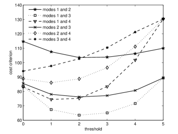
Figure 1: Dependence of the cost criterion on the threshold

The obtained results illustrate the necessity of the input control and possibility to reduce the cost of the system operation by means of the threshold type control.

Now let us vary the buffer size $K$ from 1 to 100. Table 2 contains the optimal criterion value for the cases with and without control ($C^{*}$ and $C_{r}$, $r=\overline{1,4}$), the optimal threshold $j^{*}$ and the relative profit $R$ for different buffer capacity $K$. Note that in all cases the optimal control only uses the modes with one and three active robots. The results for $K>30$ are approximately the same as for $K=30$.

Table 2: Variable Buffer Size $K$

$K$	$j^{*}$	$C^{*}$	$C_{1}$	$C_{2}$	$C_{3}$	$C_{4}$	$R$, %
1	0	147.5	244.7	233.4	187.2	258.8	21.0
2	1	96.8	199.2	174.0	128.8	194.4	24.8
3	2	79.1	172.6	140.3	105.4	160.0	24.9
4	2	68.3	158.1	121.7	94.7	140.6	27.85
5	2	63.5	149.9	110.0	89.4	130.3	28.9
6	3	60.8	144.7	102.3	86.7	124.1	29.8
7	3	59.3	141.6	97.2	85.5	120.5	30.6
8	3	58.4	138.5	93.7	85.0	118.3	31.2
9	3	57.8	137.9	91.3	84.9	117.1	31.8
10	3	57.5	137.0	89.7	85.0	116.5	32.3
20	3	57.2	137.0	86.3	87.2	120.0	33.7
30	3	57.2	137.0	86.3	87.4	123.6	33.7

Let the mean service time $b_{1}$ be varied by means of the matrix $S$ multiplication by the value $s$ which varies from 0.1 to 15. Table 3 contains the value $s$, the mean service time $b_{1}$, the optimal set of possible numbers of active robots, the optimal value of the threshold, the optimal cost criterion value and the value of the cost criterion when only one of the modes is in use (when the number of active robots is fixed), and the relative profit $R$. Note that when $s$ is equal to or grater than 15, i.e. $b_{1}$ is less than 0.04, no dynamic control is required.

Now we vary the mean time $g_{1}$ until obsolescence by the same way as it was done for the mean service time. Table 4 shows obtained results. Note that in the optimal set of modes only one and three active robots are used in all considered cases.

Consider the effect of the service time variation on the cost criterion value given that the mean service time $b_{1}$ is constant and equals to 0.657. Let the matrix $S$ of service time distribution have the form

$$S=\begin{pmatrix}-\alpha_{1}&0\\ 0&-\alpha_{2}\\ \end{pmatrix}$$

and vector ${\boldsymbol{\boldsymbol{\beta}}}=(0.9\;0.1)$.

The variance of service time is calculated as

$$var_{s}=2{\boldsymbol{\boldsymbol{\beta}}}S^{-2}{\mathbf{e}}-({\boldsymbol{\boldsymbol{\beta}}}(-S)^{-1}\mathbf{e})^{2}.$$

To maintain the mean service time $b_{1}$, the entries $\alpha_{1}$ and $\alpha_{2}$ of matrix $S$ must be related through the formula $b_{1}={\boldsymbol{\boldsymbol{\beta}}}(-S)^{-1}{\mathbf{e}}_{M}$ as

$$\alpha_{2}=\frac{0.1\alpha_{1}}{b_{1}\alpha_{1}-0.9}.$$

Note that $\alpha_{1}$ should be grater than 1.369 to keep $\alpha_{2}$ positive.

Let us vary the value of $\alpha_{1}$ from 1.521 to 9. The service time variation $var_{s}$ takes the values from 0.431 to 5.798. In the case $\alpha_{1}=1.521$ service time distribution is exponential one. In the optimal set of operation modes only one and three active robots are used. Figure 2 shows dependence of the cost criterion value on the threshold under different values of service time variation ($\alpha_{1}\in\{1.521,3,5,7,9\}$).

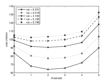
Figure 2: Dependence of the cost criterion on service time variation

But when $\alpha_{1}$ becomes larger than 4 ($var_{s}>3.415$), not the modes with one and three active robots but the modes with one and four active robots are the optimal set of exploited modes. Figure 3 shows the dependence of the cost criterion when only optimal set of modes is in use. In the figure, two lower curves correspond to the modes with one and three active robots and other curves correspond to the modes with one and four active robots.

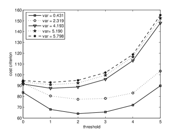
Figure 3: Dependence of the cost criterion on service time variation

Now let us vary the variance of time until obsolescence in the same way. Let the matrix $G$ have the form

$$G=\begin{pmatrix}-\alpha_{1}&0\\ 0&-\alpha_{2}\\ \end{pmatrix}$$

and $\gamma=(0.9\;0.1).$ To maintain the average time until obsolescence $g_{1}=5$, the value $\alpha_{2}$ is related to $\alpha_{1}$ as

$$\alpha_{2}=\frac{0.1\alpha_{1}}{g_{1}\alpha_{1}-0.9}.$$

We vary $\alpha_{1}$ from 0.2 to 7. Thus the variation takes the values from 25 to 449. Note that in the case $\alpha_{1}=0.2$, we get the time until obsolescence distributed exponentially. The optimal strategy consists of modes with one and three active robots in all considered cases. Figure 4 shows dependence of the cost criterion value on variation of time until obsolescence ($\alpha_{1}\in\{0.2,0.5,1,3,7\}$). Note that as the variation grows the optimal threshold decreases from 2 to 0.

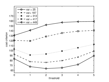
Figure 4: Dependence of the cost criterion on variation of time until obsolescence

Now let us consider the example based on real data obtained from the robot designed by INRIA Maestro team in the framework of RIAM INRIA-Canon Research Project. Data about the information delivery process by the robot to the data base was presented in the form of the text file which contained more than 65 000 timestamps defining epochs of information delivery.

This data was processed in the following way.

• Inter-arrival times were computed.

• The obtained sample was censored: very long intervals, which actually correspond to the periods when the crawling process was stopped due to some reason, are deleted from the sample.

• The obtained sample was transformed into two samples in such a way as the very short inter-arrival times were deleted from the initial sample and the corresponding information about the number of successively deleted intervals was placed into another sample. As the result of these manipulations, we stated that the arrival process is the batch arrival process. One sample defines the intervals between the epochs of batches arrival, the second sample defines the number of the information units in the corresponding batch. By information units we mean either the principal part of a Web page (e.g., Web page main html file) or its embedded resources (e.g., image and audio files).

• Based on the second sample, distribution of the number of the information units in a batch was computed as follows. The size of a batch varies in the interval $[1,8]$ and probabilities $d_{k}$ that the batch size is equal to $k=1,2,\dots,8$ are the following: $d_{1}=0.040445227$, $d_{2}=0.18404232$, $d_{3}=0.26405114$, $d_{4}=0.5057307$, $d_{5}=8.8163983\cdot 10^{-4}$, $d_{6}=7.7143486\cdot 10^{-4}$, $d_{7}=0.0018734847$, $d_{8}=0.00220405$. The mean batch size is equal to 3.263389905223716.

• Based on the first sample, we computed estimation of the mean value of an interval between arrivals of batches as 212.03, estimation of the variance of such an interval as 51352.38 and the estimations of lag-$k$ correlation of inter-arrival times for $k$ equal to $1,2,\dots,6$ are given by 0.622; 0.574; 0.555; 0.537; 0.523; 0.507. Thus, the flow defined by a sample under study has slowly decreasing correlation. In this situation, it is reasonable to apply method by Diamond and Alfa [4] oriented to such flows.

• As the result, the process of the arrival of the batches was defined by the $MAP$ which is characterized by the matrices

  $$D_{0}=\begin{pmatrix}-0.0038&0\\ 0&-0.0066\\ \end{pmatrix},\;$$

  $$D_{1}=A,\;A=\begin{pmatrix}0.0037&6.58\cdot 10^{-5}\\ 1.3\cdot 10^{-4}&0.0064\\ \end{pmatrix}.$$

• Based on this $MAP$ of batches and information about the batch size distribution, the $BMAP$ of Web pages is constructed. It is defined by the matrices $D_{0}$ and $D_{k}=d_{k}A,\;k=\overline{1,8}.$

To estimate a Web page service time distribution, the following information about the size of an arbitrary information unit delivered by a crawler (content size) in the used data base was exploited: the mean content size is equal to 49207.0356 bytes, the mean squared content size is equal to 2.0527E+11, and the mean cubed content size is equal to 2.5773E+18. Based on this information, the service time distribution of a Web page was described, up to some normalizing constant defined by the content processing rate (in our application the processing rate is constant), by the hyper-exponential distribution which is the partial case of the $PH$ distribution defined by the vector ${\boldsymbol{\beta}}=(0.0057\,0.9943)$ and by sub-generator

$$S=\begin{pmatrix}-0.0014&0\\ 0&-0.2409\\ \end{pmatrix}.$$

The mean service time is 8.2. The squared coefficient of variation of the service time distribution is equal to 86.03. Because the exponential distribution has the squared coefficient of variation equal to 1, is is clear that this distribution can not be considered as a good approximation of the service time distribution.

We assume that the system has four available operation modes. The buffer capacity is $K=20$.

When the $r$ robots are activated, the $BMAP$-input is described by the matrices ${\mathcal{D}}_{k}^{(r)}$,

$${\mathcal{D}}_{k}^{(r)}=rD_{k},\quad k=\overline{0,8},r=\overline{1,4},$$

where the matrices $D_{k},\quad k=\overline{0,8},$ are defined above. The intensities $\lambda^{(r)}$ of the $BMAP$ when $r$ robots are used, $r=\overline{1,4},$ are as follows: $\lambda^{(1)}=0.0153$, $\lambda^{(2)}=0.0307$, $\lambda^{(3)}=0.046$, $\lambda^{(4)}=0.061$.

The distribution of a Web page obsolescence time is exponentially distributed with parameter 0.0005, i.e., the mean time until obsolescence is equal to 2000.

The cost criterion coefficients are taken as $c_{loss}=200$, $c_{obs}=250$, $a=3$, $c_{rob}=20$, $c_{star}=600.$

The cost criterion values $C_{r}$ when $r,$ $r=\overline{1,4},$ robots are always activated are given by $C_{1}=666.28$, $C_{2}=657.07$, $C_{3}=639.03$ and $C_{4}=621.25$. When all four modes of operations are exploited the optimal cost criterion value is 563.51 and the optimal set of thresholds is [2,2,2], i.e., the optimal strategy assumes that four robots should be active until the number of Web pages in the system does not exceed 2. When the number of Web pages in the system exceeds 2, three robots should be deactivated and only one robot should be active.

Table $5$ contains the optimal values of the cost criterion for the different combinations of operation modes.

Table $5$: The Values of the Optimal Cost Criterion for the Fixed Combination of Operation Modes possible numbers of active robots Optimal thresholds Optimal value of the cost criterion 1 – 666.28 2 – 657.07 3 – 639.03 4 – 621.25 1,2 0 624.97 1,3 0 591.72 1,4 2 563.51 2,3 1 622.81 2,4 2 593.29 3,4 3 609.66 1,2,3 0,0 591.72 1,2,4 2,2 563.51 1,3,4 2,2 563.51 2,3,4 2,2 593.29 1,2,3,4 2,2,2 563.51

The relative profit of operation mode control exceeds 9% comparing to the case when no control is applied and all four robots are always active.

8 Conclusion

In this paper we provide performance evaluation and optimization of the crawling part of a Web search engine. We model the crawler with a finite buffer, monotonically controlled arrival rate (controlled number of crawling robots), and with stochastically bounded waiting time. The system is considered under rather general assumptions about the arrival process, service and obsolescence time distributions. Stationary distribution of the system state, sojourn time distribution and main performance measures of the system are calculated under any fixed set of thresholds defining the control strategy. This allows us to reduce the problem of optimal control to minimization of a known function of several integer variables.

Numerical results are presented. They show that the dynamic input control can give essential profit. Effects of buffer size changes and changes of average service and obsolescence times and their variances are investigated. In particular, we illustrate that the assumption about the exponential distribution of service and obsolescence times can give poor estimation of the system performance measures and optimal values of the thresholds when actually these times have high variation.

The model has been applied to the performance evaluation and optimization of the crawler designed by INRIA Maestro team in the framework of the RIAM INRIA-Canon research project.

]

References

- [1] J. Artalejo, D.S. Orlovsky, and A.N. Dudin, ”Multiserver retrial model with variable number of active servers”, Computers and Industrial Engineering, vol. 28, pp. 273-288, 2005.
- [2] S. Asmussen, O. Nerman and M. Olsson, ”Fitting Phase-Type Distributions via the EM Algorithm”, Scandinavian Journal of Statistics, vol. 23, pp. 419-441, 1996.
- [3] T. Crabill, ”Optimal control of a service facility with variable expenential service times and constant arrival rate”, Management Science, vol. 9, pp. 560-566, 1972.
- [4] J.E. Diamond and A.S. Alfa, ”On approximating higher order s with s of order two”, Queueing Systems, vol. 34, pp. 269-288, 2000.
- [5] A. Dudin, ”Optimal multi-threshold control for a queue with service modes”, Queueing Systems, vol. 30, pp. 273-287, 1998.
- [6] A.N. Dudin and V.I. Klimenok, ”Optimal admission control in a queueing system with heterogeneous traffic”, Operations Research Letters, vol. 28, pp. 108-118, 2003.
- [7] A. Graham, Kronecker Products and Matrix Calculus with Applications, Chichester: Ellis Horwood, 1981.
- [8] C.S. Kim, V.I. Klimenok, A.A. Birukov and A.N. Dudin, ”Optimal multi-threshold control by the BMAP—SM—1 retrial system”, Annals of Operations Research, vol. 141, pp. 193–210, 2006.
- [9] V.I. Klimenok, C.S. Kim, D.S. Orlovsky and A.N. Dudin, ”Lack of invariant property of Erlang model”, Queueing Systems, vol. 49, pp. 187-213, 2005.
- [10] D. M. Lucantoni, ”New results on the single server queue with a batch Markovian arrival process,” Communications in Statistics-Stochastic Models, vol. 7, pp. 1-46, 1991.
- [11] M. Neuts, Matrix-geometric solutions in stochastic models, Baltimore, USA: The Johns Hopkins University Press, 1981.
- [12] A. Pattavina and A. Parini A., ”Modelling voice call inter-arrival and holding time distributions in mobile networks”, in: Performance Challenges for Efficient Next Generation Networks - Proc.of 19th International Teletraffic Congress, Aug.-Sept. 2005, pp. 729-738.
- [13] J. Talim, Z. Liu, Ph. Nain and E. G. Coffman, Jr., ”Controlling the Robots of Web Search Engines”, Performance Evaluation Review, vol. 29. No 1, pp. 236-244, 2001.
- [14] H. Tijms, ”On the optimality of a swith-over policy for controlling the queue size in a queue with variable service rates”, Lecture Notes in Computer Sciences, vol. 40. pp. 236-242, 1976.
- [15] C.E. Wells, ”Determining the Future Costs of Lifetime Warranties”, IIE Transactions, vol. 19, pp. 178-181, 1987.
Table 3: Variable Mean Service Time