Quantum Storage of a Photonic Polarization Qubit in a Solid

Abstract

We report on the quantum storage and retrieval of photonic polarization quantum bits onto and out of a solid state storage device. The qubits are implemented with weak coherent states at the single photon level, and are stored for $500\,\mathrm{ns}$ in a praseodymium doped crystal with a storage and retrieval efficiency of $10\,\mathrm{\%}$, using the atomic frequency comb scheme. We characterize the storage by using quantum state tomography, and find that the average conditional fidelity of the retrieved qubits exceeds $95\,\%$ for a mean photon number $\mu=0.4$. This is significantly higher than a classical benchmark, taking into account the Poissonian statistics and finite memory efficiency, which proves that our device functions as a quantum storage device for polarization qubits, even if tested with weak coherent states. These results extend the storage capabilities of solid state quantum memories to polarization encoding, which is widely used in quantum information science.

The ability to transfer quantum information in a coherent, efficient and reversible way from light to matter plays an important role in quantum information science Hammerer2010 . It enables the realization of photonic quantum memories (QM) simon2010 which are required to render scalable elaborate quantum protocols involving many probabilistic processes that have to be combined. A prime example is the quantum repeater Briegel1998 ; Duan2001 ; Sangouard2011 , where quantum information can be distributed over very long distances. Other applications include quantum networks Kimble2008 , linear optics quantum computation Kok2007 , deterministic single photon sources Matsukevich2006 and multiphoton quantum state engineering.

Proof of principle experiments demonstrating photonic QMs have been reported in different atomic systems such as cold Chaneliere2005 ; Chou2005 ; Simon2007c ; Choi2008 ; Zhao2009 ; Radnaev2010 ; Zhang2011 and hot atomic gases Julsgaard2004 ; Eisaman2005 ; Reim2011 ; Hosseini2011 , single atoms in cavities Specht2011 and solid state systems Riedmatten2008 ; Hedges2010 . In recent years, solid state atomic ensembles implemented with rare-earth doped solids have emerged as a promising system to implement QMs. They provide a large number of atoms with excellent coherence properties naturally trapped into a solid state system. In addition, they feature a static inhomogeneous broadening that can be shaped at will, enabling new storage protocols with enhanced storage properties (e.g. temporal multiplexing) Kraus2006 ; Afzelius2009 . Finally, some of the rare-earth doped crystals (e.g. praseodymium and europium doped crystals) possess ground states with extremely long coherence times Longdell2005 ($>$ seconds), which hold promise for implementing long lived solid state quantum memories.

Recent progress towards solid state QMs include the storage of weak coherent pulses at the single photon level Riedmatten2008 ; Sabooni2010 ; Chaneliere2010 ; Lauritzen2010 , the quantum storage of coherent pulses with efficiency up to $70\,\%$ Hedges2010 , the spin state storage of bright coherent pulses Longdell2005 ; Afzelius2010 and the storage of multiple temporal modes in one crystal Usmani2010 ; Bonarota2011 . Very recently, these capabilities have been extended to the storage of nonclassical light generated by spontaneous down conversion, leading to the entanglement between one photon and one collective atomic excitation stored in the crystal Clausen2011 ; Saglamyurek2011 , and entanglement between two crystals Usmani2011 .

All previous experiments with solid state QMs have been so far limited to the storage of multiple modes using the time degree of freedom, e.g. time bin or energy time qubits. However, quantum information is very often encoded in the polarization states of photons, which provide an easy way to manipulate and analyze the qubits. Extending the storage capabilities of solid state QMs to polarization encoded qubits would thus bring much more flexibility to this kind of interface. Unfortunately, storing coherently polarization states is not straightforward in rare-earth doped crystals. The main difficulty is that these crystals have in general a strongly polarization dependent absorption. Storing directly a polarization qubit in such a system would result in a severely degraded fidelity of the retrieved qubits.

In this paper, we report on the storage and retrieval of a photonic polarization qubit into and out of a solid state quantum storage device with high conditional fidelity. The photonic qubits are implemented with weak coherent pulses of light, with a mean photon number $\mu$ from $0.01$ to $36$. We measure the conditional fidelity simon2010 of the storage and retrieval process (i.e. assuming that a photon was re-emitted) and compare it to classical benchmarks. With this procedure, we can show that our crystal behaves as a quantum storage device, even if tested with classical, weak coherent pulses. We overcome the difficulty of anisotropic absorption by splitting the polarization components of the qubit and storing them in two spatially separated ensembles within the same crystal Matsukevich2004 ; Chou2007 ; Choi2008 .

Our memory is implemented using a $3\,\mathrm{mm}$ long $\mathrm{Pr^{3+}:Y_{2}SiO_{5}}$ crystal ($0.05\,\%$). The relevant atomic transition connects the $\mathrm{{}^{3}H_{4}}$ ground state to the $\mathrm{{}^{1}D_{2}}$ excited state and has a wavelength of $605.977\,\mathrm{nm}$. Each state has three hyperfine sublevels as shown in Fig. 1. The measured maximal optical depth at the center of the $5\,\mathrm{GHz}$ inhomogeneous line is $\mathrm{OD}=7$. We use the Atomic Frequency Comb (AFC) scheme to store and retrieve the qubits Afzelius2009 . This requires to shape the inhomogeneous absorption profile into a series of periodic and narrow absorbing peaks, placed in a wide transparency window. This creates a frequency grating and when a photon is absorbed by the comb, it will be diffracted in time and re-emitted after a pre-determined time $t_{S}=1/\Delta$, where $\Delta$ is the spacing between absorption peaks.

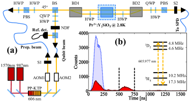
Figure 1: (Color online) (a) Experimental setup. The preparation beam and the qubit beam are derived from the same laser at $606\,\mathrm{nm}$. Both beams are amplitude and frequency modulated using an acousto-optic modulator (AOM). The polarization of the preparation beam is set to $45$ degrees, while the polarization of the qubit beam can be set arbitrarily with a half wave plate (HWP) and a quarter wave plate (QWP). The qubit beam is attenuated down to the single photon level using neutral density filters (NDF). The two beams are recombined at a beam splitter (BS) and sent to the storage device which is composed of a $\mathrm{Pr^{3+}:Y_{2}SiO_{5}}$ crystal cooled to $2.8\,\mathrm{K}$, two beam displacer (BD) and two HWP. The light released by the memory is then sent to a polarization analyzer composed of a HWP, a QWP and a polarization beam splitter (PBS), before being detected with a single photon detector (SPD). The two mechanical shutters (S1 and S2) are used to suppress optical noise from the preparation beam and to protect the SPD. (b) Storage and retrieval of a weak $|V\rangle$ qubit with duration $140\,\mathrm{ns}$ and $\mu=0.4$. The temporal histogram of the detection without (dotted line,empty pit) and with (solid line) AFC is shown. The dashed lines around the AFC echo show the detection window. Inset: Level scheme of $\mathrm{Pr^{3+}:Y_{2}SiO_{5}}$ with the dashed arrows showing the relevant transition for photon absorption and re-emission.

Our experimental apparatus is described in Fig. 1. The laser source to generate light at $606\,\mathrm{nm}$ is based on sum frequency generation (SFG) in a PP-KTP waveguide (AdVR corp) from two amplified laser diodes at $1570\,\mathrm{nm}$ (Toptica, DL 100 and Keopsys fiber amplifier) and $987\,\mathrm{nm}$(Toptica, TA pro). With input power of $370\,\mathrm{mW}$ and $750\,\mathrm{mW}$ for the $987\,\mathrm{nm}$ laser and $1570\,\mathrm{nm}$ laser, respectively, we achieve an output power of $90\,\mathrm{mW}$ at $606\,\mathrm{nm}$. Taking into account the $30\,\%$ coupling efficiency of both beams into the waveguide, we obtain a SFG efficiency of $\sim 350\,\mathrm{\%W^{-1}}$. The beam is then split in two parts, one which will be used for the memory preparation (preparation beam) and one to prepare the weak pulses to be stored (qubit beam). In each path, the amplitude of the light is modulated with an acousto-optic modulator (AOM) in a double pass configuration, in order to create the required sequence of pulses for the preparation of the memory and of the polarization qubits. The radio-frequency signals used to drive the AOMs are generated by an arbitrary waveform generator ($500\,\mathrm{Msample/s}$, $200\,\mathrm{MHz}$, $\,\mathrm{1GB}$ internal memory, PXIe module and ProcessFlow software from Signadyne). After the AOMs, both beams are coupled to a polarization maintaining optical fiber and sent to another optical table where the cryostat is located.

The crystal is cooled down to $2.8\,\mathrm{K}$ in a cryofree cooler (Oxford Instruments V14). After the fibers, the preparation beam is collimated to a diameter of around $600\,\mathrm{\mu m}$ with a telescope and sent to the storage device. Right before the cryostat, a beam displacer (BD1) splits the two polarization components of the incoming light onto two parallel spatial modes separated by $2.7\,\mathrm{mm}$, co-propagating through the crystal. To ensure equal power in both spatial modes, the polarization of the preparation beam is set to $45$ degrees. After BD1, the polarization of the horizontal beam (lower beam in Fig.1) is rotated by $90$ degrees using a HWP such that both beams enter the crystal with the same polarization which is parallel to the D2 axis of the crystal, which maximizes the absorption. The qubit beam is strongly attenuated by a set of fixed and variable neutral density filters (NDF), and $\mu$ before BD1 was varied from $0.01$ to $36$. After the NDF, arbitrary polarization qubits are prepared, using a quarter (QWP) and a half wave plate (HWP). The qubits are then overlapped to the preparation beam at a beam splitter (BS). After the cryostat, we rotate back the polarization of the lower beam and the two spatial modes are combined again at a second beam displacer (BD2). The two path between BD1 and BD2 form an interferometer with very high passive stability Chou2007 ; Choi2008 .

After the interferometer, the transmitted and retrieved light enters the polarization analysis stage, composed of a QWP, a HWP and a polarization beam splitter (PBS), which allow us to measure the polarization in any basis. The transmitted beam at the PBS is coupled in a multimode fiber and sent to a Silicon avalanche photodiode Single Photon detector (SPD, model Count, Laser Components). The electronic signal from the SPD is finally sent to a time stamping card (PXIe card from Signadyne) in order to record the arrival time histogram. The mean photon number $\mu$ is determined by measuring the detection probability per pulse $p_{det}$ when no atoms are present (i.e. with the laser $60\,\mathrm{GHz}$ off resonance), and backpropagating before BD1 taking into account the detection efficiency ($\eta_{D}=50\,\%$) and the transmission from before BD1 to the detector ($\eta_{t}=40\,\%$). The preparation beam and the qubits are sent sequentially towards the crystal. The total experimental sequence lasts $3$ seconds, during which the preparation lasts $1\,\mathrm{s}$. During the next $2$ seconds $10^{5}$ weak pulses are prepared, stored and retrieved at a rate of $50\,\mathrm{kHz}$.

In order to create the AFC, we first create a wide transparency window within the $5\,\mathrm{GHz}$ inhomogeneous profile. This is achieved by sending a series of pulses of duration $1.1\,\mathrm{ms}$, during which the frequency of the light is swept linearly over a range of $12\,\mathrm{MHz}$. The AFC is then created using the burn back procedure introduced in Ref. Nilsson2004 , i.e. by illuminating the sample with short pulses of duration $2\,\mathrm{ms}$, while shifting the frequency of the light by $-27\,\mathrm{MHz}$ with respect to the center of the pit. Four burn back pulses are sent with different frequencies separated by the comb spacing, leading to a 4-tooth comb.

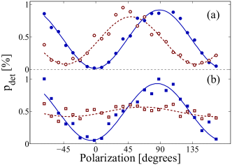
Figure 2: (Color online) (a) Measured detection probability ($p_{det}$) as a function of the polarizer angle, for $|V\rangle$ (filled circles) and $|D\rangle$ (open circles) input polarization qubits, with $\mu=0.4$. The fitted raw visibilities are $(97\pm 0.5)\,\%$ and $(83\pm 2)\,\%$, respectively. (b) $p_{det}$ as a function of polarization angle for $|R\rangle$ polarization qubit input, with (filled squares, $(89\pm 2)\,\%$) and without (open squares, $(15\pm 3)\,\%$) QWP inserted before the polarizer.

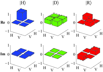
Figure 3: (Color online) Quantum state tomography. Reconstructed density matrices of the retrieved qubits for $|H\rangle$, $|D\rangle$ and $|R\rangle$ input qubits, with $\mu=0.4$ . No background has been subtracted.

Input State	Fidelity	Input State	Fidelity
$|H\rangle$	0.982 $\pm$ 0.003	$|V\rangle$	0.983 $\pm$ 0.002
$|D\rangle$	0.968 $\pm$ 0.005	$|A\rangle$	0.938 $\pm$ 0.009
$|R\rangle$	0.954 $\pm$ 0.007	$|L\rangle$	0.926 $\pm$ 0.01

Table 1: Raw conditional fidelities for 6 different polarization input states. For this measurement, $\eta_{M}$ varied between 8 $\%$ and 10 $\%$. The errors have been obtained using Monte Carlo simulation taking into account the statistical uncertainty of photon counts and a technical error reflecting slow drifts in our systems, and estimated from the residuals from the fit of Fig.2 and similar curves.

As a first experiment, we verified that a complete set of qubit distributed over the Poincaré sphere could be stored and retrieved in the AFC. We set the storage time to $500\,\mathrm{ns}$ and we used the following input states: $|H\rangle$,$|V\rangle$, $|D\rangle=\frac{1}{\sqrt{2}}(|H\rangle+|V\rangle)$, $|A\rangle=\frac{1}{\sqrt{2}}(|H\rangle-|V\rangle)$, $|R\rangle=\frac{1}{\sqrt{2}}(|H\rangle+i|V\rangle)$ and $|L\rangle=\frac{1}{\sqrt{2}}(|H\rangle-i|V\rangle)$. Fig.1 (b) shows the experimental storage of a $|V\rangle$ qubit encoded onto a pulse of duration $140\,\mathrm{ns}$ (FWHM) and with $\mu=0.4$. Similar curves are obtained for the other states, and the average storage and retrieval efficiency is $\eta_{M}=(10.6\pm 2.3)\,\%$. In order to test that the coherence between the $|H\rangle$ and $|V\rangle$ components of the qubits is preserved during the storage and retrieval, we then recorded the number of counts in the retrieved pulses when rotating the detection polarization basis using a HWP, for various input states. In Fig. 2 (a), the curves obtained for $|V\rangle$ and $|D\rangle$ are shown. We observe interference fringes, with a raw fitted visibility of $(97\pm 0.5)\,\%$ for the $|V\rangle$ qubit, and $(83\pm 2)\,\%$ for the $|D\rangle$ qubit. In the case of a perfect circular $|R\rangle$ qubit, we should observe no dependance on the HWP angle when no QWP is inserted. The interference should be restored however, when a QWP is inserted before the HWP, which turns circular polarization into a linear one. The results are shown in Fig. 2 (b). We indeed observe a strongly reduced visibility without the HWP ($(15\pm 3)\,\%$), while a fringe with a high visibility of $(89\pm 2)\,\%$ is obtained with the QWP. The residual visibility without the QWP may be due to a non perfect preparation of the $|R\rangle$ state. The non perfect visibility for the $|D\rangle$ and $|R\rangle$ is mostly due to small phase fluctuations engendered by mechanical vibrations from the cryostat. Indeed, we observe similar visibilities for bright pulses out of resonance with the atomic transition. These results show that the phase between the two polarizations components is almost perfectly preserved in the storage and retrieval process, and is preserved to a high degree in our combined interferometer and memory setup, for various polarization input states.

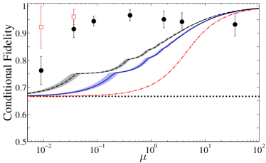
Figure 4: (Color online) Average fidelity measured as a function of the mean number of photon per pulse $\mu$. The fidelity is measured by quantum state tomography and is the average of $3$ input states $|V\rangle$, $|D\rangle$, and $|R\rangle$. Filled circles are experimental data without any background subtraction. Empty squares correspond to dark count subtracted fidelities. The error takes into account statistical uncertainty of photon counts, technical errors and standard deviation of fidelities for the 3 polarizations. The various lines correspond to classical thresholds for different situations. The horizontal line is the limit of $2/3$ for single qubits (N=1). The dashed-dotted line corresponds to Eq.1 where the Poissonian distribution of photon number is taken into account. Finally, the two other lines correspond to the cases where the finite storage efficiency is taken into account. The solid line corresponds to $\eta=(10\pm 2)\,\%$. Measured $\eta_{M}$ are between $8$ and $10\,\%$ for all points. The dashed line corresponds to $\eta=\eta_{M}\eta_{t}\eta_{D}=2\,\%$. For $\mu>1$, an additional ND filter is placed before the detector to avoid saturation effects.

In order to better characterize the quality of the storage process, we reconstruct the density matrix of the retrieved qubits using quantum state tomography James2001 , for the complete set of qubits described above, with $\mu=0.4$. The reconstructed output density matrices $\rho_{out}$ for $|H\rangle$, $|D\rangle$ and $|R\rangle$ are shown in Fig 3. From the matrices $\rho_{out}$, we can then estimate the conditional fidelity of the output states with respect to the target state $F^{c}_{|\psi\rangle}=\langle\psi|\rho_{out}|\psi\rangle$. The values for the complete set of inputs are listed in Table 1. We find a mean fidelity of $F^{c}_{mean}=(96\pm 2)\,\%$. We emphasize that this value is a lower bound for the conditional fidelity, since it is calculated with respect to a target state and also takes into account imperfections in the preparation of the qubits.

Finally, in order to assess the quantum nature of the storage, we determine the average fidelity as a function of $\mu$, and compare it with the best obtainable fidelity using a purely classical method consisting of measuring the state and storing the result in a classical memory. It has been shown that for a state containing $N$ qubits, the best classical strategy leads to a fidelity of $F_{c}=(N+1)/(N+2)$ Massar1995 , leading to the well known fidelity of $2/3$ for $N=1$. If the qubit is encoded in a weak coherent state, as it is the case in our experiment, one has to take into account the Poissonian statistics of the number of photons Specht2011 , and the classical fidelity is given by:

$$F_{class}(\mu)=\sum_{N\geq 1}\frac{N+1}{N+2}\times\frac{P(\mu,N)}{1-P(\mu,0)},$$ (1)

where $P(\mu,N)=e^{-\mu}\mu^{N}/N!$. This is valid for the case of a memory with unity efficiency. If $\eta_{M}<1$, the classical memory could use a more elaborate strategy to take advantage of finite efficiency in order to gain more information about the input quantum state Specht2011 . For example the classical memory could give an output only when the number of photons per pulse is high, and hence estimate with better fidelity the quantum state (See appendix A). The different curves corresponding to the discussed cases are plotted in Fig. 4 as a function of $\mu$. The points correspond to experimental data. Measured $F^{c}_{mean}$ are significantly higher than the classical fidelity, for most of the photon numbers tested. This proves that our device performs as a quantum storage device for polarization qubits, even if tested with weak coherent states. We observe that the measured raw fidelity decreases for $\mu<0.1$. This is mainly due to the dark count of the SPD, as high fidelities can be recovered by subtraction of this background (open squares). We also observe that when $\mu$ becomes too large ($\mu\geq 3.5$ in our case), the measured fidelity is not sufficient to be in the quantum regime. This confirms that very low photon numbers are required to test the quantum character of QMs with weak coherent states. To our knowledge, it is the first time that an ensemble based memory has been characterized using this criteria.

The storage time in our experiment is limited by the minimal achievable width of the AFC peaks ($<$600 kHz), which is in turn fully limited by the linewidth of our unstabilized laser. Peaks as narrow as $30\,\mathrm{kHz}$ have been created in $\mathrm{Pr^{3+}:Y_{2}SiO_{5}}$ using a frequency stabilized laser Hetet2008a , which should allow a storage time in the excited state of about 10 $\mathrm{\mu s}$. This should also allow the storage of multiple polarization qubits in the time domain. In order to increase the storage time and to achieve on demand read out with an AFC, the optical excitations should be transferred to long lived spin excitation as demonstrated for bright pulses in Afzelius2010 .

We have demonstrated the quantum storage and retrieval of polarization qubits implemented with weak coherent pulses at the single photon level, in a solid state storage device. The conditional fidelity of the storage and retrieval is $>95\,\%$, significantly exceeding the classical benchmark calculated for weak coherent pulses and finite memory efficiency. We thus show that solid state QMs are compatible with photonic polarization qubits, which are widely used in quantum information science. This significantly extends the storage capabilities of these types of memories. By combining the time and polarization degrees of freedom one could readily double the number of modes that can be stored in the memory and create quantum registers for polarization qubits. Using these resources, it may also be possible to design a quantum memory for complex light states such as hyperentangled states.

We note that related results have been obtained by two other groups Saglamyurek2011a ; Clausen2012 .

We thank Stephan Ritter and Antonio Acin for interesting discussions regarding the classical benchmark, and the company Signadyne for technical support. Financial support by the CHIST-ERA European project QScale and by the ERC Starting grant QuLIMA is acknowledged.

Appendix A Conditional Fidelity using Classical State Estimation for Weak Coherent States

In this section, we give more details on the calculation of the classical benchmark presented in Fig. $4$ of the main manuscript. The general idea is to estimate what is the best efficiency that can be obtained using a classical method. In particular, we consider a measure and prepare strategy where the user performs a classical state estimation on the input qubit, stores the result in a classical memory and prepares a new qubit according to the result obtained. The maximum achievable classical fidelity for a state with a fixed photon number $N$ is known to be Massar1995

$$F=\frac{N+1}{N+2}.$$

If one tests a memory with a true single photon input then the classical bound is ${2}/{3}$. If one uses weak coherent states then one has to consider the finite probability of having more than one photon. A pulse of light with mean photon number ${\mu}$ has a probability distribution of a Poissonian, given by

$$P({\mu},N)=\mathrm{e}^{-{\mu}}\,\frac{{\mu}^{N}}{N}.$$

Then, the maximum achievable fidelity becomes a weighted sum over $N$ of the fidelity for a given $N$ where the weight is given by the Poissonian statistics of the input Specht2011 . We state this below as

$$F=\sum_{N\geq 1}^{\infty}\;\frac{N+1}{N+2}\;\frac{P({\mu},N)}{1-P({\mu},0)}.$$ (2)

This formula is valid if one assumes that the quantum memory has a storage and retrieval efficiency $\eta_{M}=1$. If $\eta_{M}<1$, a more sophisticated classical strategy could simulate non-unit efficiency by only giving a result for high photon number $N$, resulting in a higher achievable fidelity, as suggested in Specht2011 . We consider that the classical measure and prepare strategy has an efficiency of 1, but we define the effective classical efficiency $\eta_{C}$ as the probability that the classical device gives an output qubit, if it has received at least one photon as input:

$$\eta_{C}=\frac{P_{\mathrm{out}}}{1-P(\mu,0)}.$$

where

$$P_{\mathrm{out}}=\sum_{N\geq N_{\mathrm{min}}+1}P(\mu,N).$$

Note that the photon number statistics of the output qubit is not relevant in our case, since we use non photon number resolving detectors. The classical memory gives a result for some threshold photon number $N_{\mathrm{min}}+1$ and above, and no result for $N$ lower than this. It is important to note that for the above there exists only certain $\eta_{\mathrm{C}}$ for a given mean photon number $\mu$. Hence, not all quantum efficiencies can be simulated. A more general form of $P_{\mathrm{out}}$ which allows for arbitrary number and hence efficiency is the following

$$P_{\mathrm{out}}=\gamma\;+\sum_{N\geq N_{\mathrm{min}}+1}P(\mu,N).$$

where now the memory gives a result for $N_{\mathrm{min}}$ with a probability of $\gamma$, with the condition $\gamma\leq P(\mu,N_{\mathrm{min}})$.

The efficiency is then

$$\eta_{C}=\frac{\gamma\;+\sum_{N\geq N_{\mathrm{min}}+1}\,P(\mu,N)}{1-P(\mu,0)}.$$ (3)

We now assume that $\eta_{M}=\eta_{C}$ and $N_{\mathrm{min}}$ is obtained as follows

$$N_{\min}=\mathrm{min}\,i:\sum_{N\geq i+1}P(\mu,N)\leq(1-P(\mu,0))\,\eta_{M}.$$ (4)

Figure 5 shows a graphical representation of obtaining $N_{\text{min}}$.

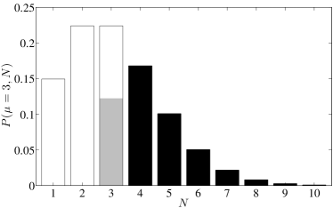
Figure 5: An example of obtaining $N_{\mathrm{min}}$. Plotted above is the probability distribution for a coherent state of $\mu=3$. The target efficiency here is $50\%$. For this target efficiency $N_{\text{min}}=3$, found using Equation 4. The grey shaded part of bar $N=3$ plus the black bars $N\geq 4$ equate to the $50\%$ target efficiency.

The maximum achievable classical fidelity using the above described strategy is then

$$F_{\mathrm{class}}=\frac{\left(\displaystyle\frac{N_{\mathrm{min}}+1}{N_{\mathrm{min}}+2}\right)\gamma+\displaystyle\sum_{N\geq N_{\mathrm{min}}+1}\displaystyle\frac{N+1}{N+2}P(\mu,N)}{\gamma+\displaystyle\sum_{N\geq N_{\mathrm{min}}+1}P(\mu,N)},$$ (5)

where $\gamma$ and $N_{\mathrm{min}}$ are obtained from Equations (3, 4). Figure 6 shows the fidelity as a function of mean photon number $\mu$ for various efficiencies $\eta$.

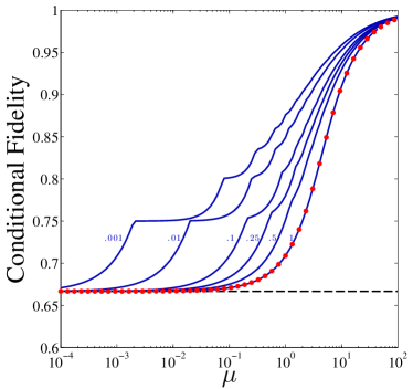
Figure 6: Maximum achievable fidelity using a classical memory as a function of mean photon number $\mu$ for different memory efficiencies $\eta$ (Eq. 3). The cases shown are $\eta~{}=~{}\{0.001,0.01,0.1,0.25,0.5,1\}$. The solid lines are calculated using Equation 5, the dots are calculated using Equation 2. It is seen that for $\eta=1$, Equation 5 reduces to Equation 2. The dashed line is for the single photon case $N=1$.

Note that the classical memory could also in principle take advantage of the optical loss and the finite detection efficiencies in the experiment to increase the maximal classical fidelity. In that case, we would have $\eta_{C}=\eta_{M}\eta_{t}\eta_{D}$, where $\eta_{t}$ is the optical transmission from the quantum memory to the detector and $\eta_{D}$ is the detection efficiency of the SPD. For our experiment, we have $\eta_{M}=0.1$, $\eta_{t}=0.4$ and $\eta_{D}=0.5$ such that in that case $\eta_{C}=0.02$.

References

- (1) K. Hammerer, A. S. Sørensen, and E. S. Polzik, Rev. Mod. Phys. 82, 1041 (2010).
- (2) C. Simon et al., The European Physical Journal D - Atomic, Molecular, Optical and Plasma Physics 58, 1 (2010-05-01).
- (3) H.-J. Briegel, W. Dür, J. I. Cirac, and P. Zoller, Phys. Rev. Lett. 81, 5932 (1998).
- (4) L.-M. Duan, M. D. Lukin, J. I. Cirac, and P. Zoller, Nature 414, 413 (2001).
- (5) N. Sangouard, C. Simon, H. de Riedmatten, and N. Gisin, Rev. Mod. Phys. 83, 33 (2011).
- (6) H. J. Kimble, Nature 453, 1023 (2008).
- (7) P. Kok et al., Rev. Mod. Phys. 79, 135 (2007).
- (8) D. N. Matsukevich et al., Phys. Rev. Lett. 97, 013601 (2006).
- (9) T. Chanelière et al., Nature 438, 833 (2005).
- (10) C. W. Chou et al., Nature 438, 828 (2005).
- (11) J. Simon, H. Tanji, J. K. Thompson, and V. Vuletic, Phys. Rev. Lett. 98, 183601 (2007).
- (12) K. S. Choi, H. Deng, J. Laurat, and H. J. Kimble, Nature 452, 67 (2008).
- (13) B. Zhao et al., Nat Phys 5, 95 (2009).
- (14) A. G. Radnaev et al., Nat Phys 6, 894 (2010).
- (15) H. Zhang et al., Nat Photon 5, 628 (2011).
- (16) B. Julsgaard et al., Nature 432, 482 (2004).
- (17) M. D. Eisaman et al., Nature 438, 837 (2005).
- (18) K. F. Reim et al., Phys. Rev. Lett. 107, 053603 (2011).
- (19) M. Hosseini et al., Nat Phys 7, 794 (2011).
- (20) H. P. Specht et al., Nature 473, 190 (2011).
- (21) H. de Riedmatten et al., Nature 456, 773 (2008).
- (22) M. P. Hedges, J. J. Longdell, Y. Li, and M. J. Sellars, Nature 465, 1052 (2010).
- (23) B. Kraus et al., Phys. Rev. A 73, 020302 (2006).
- (24) M. Afzelius, C. Simon, H. de Riedmatten, and N. Gisin, Phys. Rev. A 79, 052329 (2009).
- (25) J. J. Longdell, E. Fraval, M. J. Sellars, and N. B. Manson, Phys. Rev. Lett. 95, 063601 (2005).
- (26) M. Sabooni et al., Phys. Rev. Lett. 105, 060501 (2010).
- (27) T. Chanelière et al., New Journal of Physics 12, 023025 (2010).
- (28) B. Lauritzen et al., Phys. Rev. Lett. 104, 080502 (2010).
- (29) M. Afzelius et al., Phys. Rev. Lett. 104, 040503 (2010).
- (30) I. Usmani, M. Afzelius, H. de Riedmatten, and N. Gisin, Nat. Commun. 1, 12 (2010).
- (31) M. Bonarota, J.-L. L. Gouët, and T. Chanelière, New Journal of Physics 13, 013013 (2011).
- (32) C. Clausen et al., Nature 469, 508 (2011).
- (33) E. Saglamyurek et al., Nature 469, 512 (2011).
- (34) I. Usmani et al., arXiv:1109.0440.
- (35) D. N. Matsukevich and A. Kuzmich, Science 306, 663 (2004).
- (36) C. W. Chou et al., Science 316, 1316 (2007).
- (37) M. Nilsson et al., Phys. Rev. B 70, 214116 (2004).
- (38) D. F. V. James, P. G. Kwiat, W. J. Munro, and A. G. White, Phys. Rev. A 64, 052312 (2001).
- (39) S. Massar and S. Popescu, Phys. Rev. Lett. 74, 1259 (1995).
- (40) G. Hétet et al., Phys. Rev. Lett. 100, 023601 (2008).
- (41) E. Saglamyurek et al., arXiv:1111.0676 (2011).
- (42) C. Clausen et al., arXiv:1201.4097 (2012).