Self-diffusion in granular gases: An impact of particles’ roughness

Anna Bodrova, Nikolai Brilliantov

Department of Physics, Moscow State University, 119991 Moscow, Russia
Department of Mathematics, University of Leicester, Leicester LE1 7RH, UK

An impact of particles’ roughness on the self-diffusion coefficient $D$ in granular gases is investigated. For a simplified collision model where the normal, $\varepsilon$, and tangential, $\beta$, restitution coefficients are assumed to be constant we develop an analytical theory for the diffusion coefficient, which takes into account non-Maxwellain form of the velocity-angular velocity distribution function. We perform molecular dynamics simulations for a gas in a homogeneous cooling state and study the dependence of the self-diffusion coefficient on $\varepsilon$ and $\beta$. Our theoretical results are in a good agreement with the simulation data.

1 Introduction

Among numerous contributions by Isaac Goldhirsch to the theory of granular fluids [10] are his pioneering works on the hydrodynamic of gas of particles with the rotational degrees of freedom [11]. We wish to dedicate this article, addressed to granular gases of rough particles, to the memory of Isaac Goldhirsch.

Granular fluids are systems composed of a large number of macroscopic particles which suffer dissipative collisions. In many respects they behave like ordinary molecular fluids and may be described by the standard tools of kinetic theory and hydrodynamics [10, 5, 14]. Among numerous phenomena, common to molecular and granular fluids, are Brownian motion, diffusion and self-diffusion [3, 4, 9, 16, 6, 2, 19]; in the latter case tracers are identical to surrounding particles. The self-diffusion coefficient $D$ has a microscopic and macroscopic (thermodynamic) meaning, e.g. [5, 6]: Microscopically, it characterizes the dependence on time of the mean-square displacement of a grain $\langle\vec{R}^{2}(t)\rangle$:

$$\langle\vec{R}^{2}(t)\rangle=6\int\limits_{0}^{t}D(t^{\prime})dt^{\prime}\,,$$ (1)

while macroscopically, it relates the macroscopic flux of tracers $\vec{J}_{s}\left(\vec{r},t\,\right)$ (the index s refers to tracers) to its concentration gradient $\vec{\nabla}n_{s}\left(\vec{r},t\,\right)$:

$$\vec{J}_{s}\left(\vec{r},t\,\right)=-D(t)\vec{\nabla}n_{s}\left(\vec{r},t\,\right)\,.$$ (2)

With the continuity equation $\frac{\partial n_{s}\left(\vec{r},t\,\right)}{\partial t}+\vec{\nabla}\vec{J}_{s}\left(\vec{r},t\,\right)=0$ the local tracers density $n_{s}\left(\vec{r},t\,\right)$ obeys the diffusion equation:

$$\frac{\partial n_{s}\left(\vec{r}\,\right)}{\partial t}=D\vec{\nabla}^{2}n_{s}\left(\vec{r}\,\right)\,.$$ (3)

If the state of a granular gas is not stationary, like, e.g. a homogeneous cooling state, the diffusion coefficient generally depends on time.

In the previous studies the self-diffusion coefficient has been calculated only for smooth particles, that is, for particles which do not exchange upon collisions the energy of their rotational motion [3, 4, 9, 6, 2, 19]. The macroscopic nature of granular particles, however, implies friction between their surfaces and hence the rotational degrees of freedom are unavoidably involved in grains dynamics.

In the present paper we analyze the impact of particles roughness on the self-diffusion in granular gases – rarified systems, where the volume of the solid fraction is much smaller than the total volume. We calculate the self-diffusion coefficient as a function of normal and tangential restitution coefficients, which we assume to be constant. We develop an analytical theory for this kinetic coefficient and perform molecular dynamics (MD) simulations. The rest of the article is organized as follows. In Sect. 2 we formulate the model, introduce the necessary notations and give the detailed description of the theoretical approach. In Sect. 3 we present the results of MD simulations and compare the numerical data with the predictions of our theory. In the last Sect. 4 we summarize our findings.

2 Calculation of the self-diffusion coefficient

2.1 Collision rules

The dissipative collisions of grains are characterized by two quantities, $\varepsilon$ and $\beta$ – the normal and tangential restitution coefficients. These coefficients relate respectively the normal and tangential components of the relative velocity between surfaces of colliding grains, $\vec{g}=\vec{v}_{12}+\frac{\sigma}{2}\left(\vec{e}\times\left(\vec{\omega}_{1}+\vec{\omega}_{2}\right)\right)$, before (unprimed quantities) and after (primed quantities) a collision [5, 21]:

$$\left(\vec{g}^{\,n}\right)^{\prime}=-\varepsilon\vec{g}^{\,n}\qquad\quad\left(\vec{g}^{\,t}\right)^{\prime}=-\beta\vec{g}^{\,t}\,.$$ (4)

Here $\vec{v}_{12}=\vec{v}_{1}-\vec{v}_{2}$ is the relative translational velocity of particles, $\vec{\omega}_{1}$ and $\vec{\omega}_{2}$ are their rotational velocities, the unit vector $\vec{e}$ is directed along the inter-center vector $\vec{r}_{12}$ at the collision instant and $\sigma$ is the diameter of particles. The normal and tangential components of $\vec{g}$ read respectively, $\vec{g}^{\,n}=\left(\vec{g}\cdot\vec{e}\,\right)\vec{e}$ and $\vec{g}^{\,t}=\vec{g}-\vec{g}^{\,n}$. For macroscopic particles the normal restitution coefficient $\varepsilon$ can vary from $0$ (completely inelastic impact) to $1$ (completely elastic collision), while the tangential coefficient $\beta$ ranges from $-1$ (absolutely smooth particles) to $+1$ (absolutely rough particles). From the conservation laws and Eqs. (4) follow the after-collision velocities and angular velocities of particles in terms of the pre-collision ones, e.g. [5, 21, 12]:

$$\vec{v}_{1,2}^{\,\prime}=\vec{v}_{1,2}\mp\frac{1+\varepsilon}{2}\vec{g}^{n}\mp\eta\vec{g}^{t}$$

$$\vec{\omega}_{1,2}^{\,\prime}=\vec{\omega}_{1,2}+\frac{2\eta}{q\sigma}\left[\vec{e}\times\vec{g}^{t}\right]\,.$$ (5)

Here $\eta\equiv\frac{q(1+\beta)}{2(1+q)}$ characterizes friction, $q=4I/m\sigma^{2}$, with $I$ and $m$ being respectively the moment of inertia and mass of particles. Although the normal and tangential restitution coefficients generally depend on the translational and rotational velocities of colliding particles and an impact geometry, e.g. [5, 20, 21, 1, 17], here we assume for simplicity that the restitution coefficients are constants.

2.2 Boltzmann equation

To compute the self-diffusion coefficient in granular gases two main approaches may be exploited – Green-Kubo approach, based on the time correlation functions of a dynamical variable (a particle velocity for the case of $D$) and Chapman-Enskog method, where the evolution of velocity distribution function is analyzed. It may be shown that these two are equivalent for the case of constant normal restitution coefficient [5, 6]; here we adopt the latter approach. First we consider the force-free granular gas in a homogeneous cooling state. We start from the Boltzmann equation for the distribution function of tracers $f_{s}(\vec{v},\vec{\omega},\vec{r},t)$,

$$\left(\frac{\partial}{\partial t}+\vec{v}_{1}\cdot\vec{\nabla}\right)f_{s}\left(\vec{v}_{1},\vec{\omega}_{1},\vec{r},t\right)=g_{2}\left(\sigma\right)I(f,f_{s})\,,$$ (6)

where $f(\vec{v},\vec{\omega},\vec{r},t)$ is the velocity distribution function of the gas particles, $g_{2}\left(\sigma\right)$ is the contact value of the pair correlation function, which accounts for the increasing collision frequency due to the excluded volume of grains and $I(f,f_{s})$ abbreviates the collision integral [5, 6, 18]:

$$I(f,f_{s})\!=\!\sigma^{2}\!\int\!d\vec{v}_{2}\!\int\!d\vec{\omega}_{2}\!\int\!d\vec{e}\Theta\left(-\vec{v}_{12}\cdot\vec{e}\,\right)\left|\vec{v}_{12}\cdot\vec{e}\,\right|\times$$

$$\Big{[}\frac{1}{\varepsilon^{2}\beta^{2}}\!f_{s}\left(\vec{v}^{\,\prime\prime}_{1},\vec{\omega}^{\,\prime\prime}_{1}\right)f\left(\vec{v}^{\,\prime\prime}_{2},\vec{\omega}^{\,\prime\prime}_{2}\right)-f_{s}\left(\vec{v}_{1},\vec{\omega}_{1}\right)f\left(\vec{v}_{2},\vec{\omega}_{2}\right)\Big{]}$$

(7)

Here $\vec{v}^{\,\prime\prime}_{1,2}$ and $\vec{\omega}^{\,\prime\prime}_{1,2}$ denote the pre-collision velocities and angular velocities of particles for the inverse collision, i.e., for the collision which ends up with $\vec{v}_{1,2}$ and $\vec{\omega}_{1,2}$, the factor $\Theta\left(-\vec{v}_{12}\cdot\vec{e}\,\right)$ selects only approaching particles, and $\left|\vec{v}_{12}\cdot\vec{e}\,\right|$ gives the length of the collision cylinder. We assume that the concentration of tracers

$$n_{s}(\vec{r},t)\equiv\int d\vec{v}_{1}\int d\vec{\omega}_{1}f_{s}(\vec{v}_{1},\vec{\omega}_{1},\vec{r},t)$$ (8)

is much smaller than the number density of the gas particles $n(\vec{r},t)=n={\rm const}$, so that tracers do not affect the velocity distribution function $f$ for the gas, which is the solution of the Boltzmann equation

$$\frac{\partial}{\partial t}f\left(\vec{v},\vec{\omega},t\right)=g_{2}\left(\sigma\right)I(f,f)$$ (9)

for the homogeneous cooling state. The collision integral in the last equation is given by Eq. (7) with the distribution function of tracers $f_{s}$ substituted by that for the gas particles $f$.

Solving the Boltzmann equation (6) for $f_{s}\left(\vec{v},\vec{\omega},\vec{r},t\right)$, which is also known as Boltzmann-Lorentz equation, one can write the diffusion flux

$$\vec{J}_{s}\left(\vec{r},t\right)=\int d\vec{v}\int d\vec{\omega}\,\vec{v}f_{s}(\vec{v},\vec{\omega},\vec{r},t)\,,$$ (10)

and then, using the macroscopic equation (2), find the diffusion coefficient as the coefficient at the concentration gradient $\vec{\nabla}n_{s}\left(\vec{r},t\,\right)$.

In a homogeneous cooling state a density of the system remains uniform, while the translational $T(t)$ and rotational $R(t)$ granular temperatures, defined through the average energies of translational and rotational motion, respectively,

$$\frac{3}{2}nT=\int\!d\vec{v}d\vec{\omega}\,\frac{mv^{2}}{2}f,\qquad\frac{3}{2}nR=\int d\!\vec{v}d\vec{\omega}\,\frac{I\omega^{2}}{2}f$$ (11)

decay with time as $\partial T/\partial t=-\zeta T$ and $\partial R/\partial t=-\zeta_{R}T$, where $\zeta$ and $\zeta_{R}$ are the translational and rotational cooling rates, e.g. [5, 21, 7, 18].

The distribution function $f\left(\vec{v},\vec{\omega},t\right)$ is close to the Maxwell distribution and the deviations from the Max-wellian are twofold. Firstly, the translational and angular velocity distributions slightly differ from the Gaussian distribution, which is accounted by the expansion of $f$ in Sonine polynomials series with respect to $\vec{v}^{\,2}$ and $\vec{\omega}^{\,2}$. Secondly, a linear velocity and spin of particles are correlated; this is quantified using an expansion in Legendre polynomials series with respect to $\theta=\widehat{\vec{v}\,\vec{\omega}}$ – the angle between the velocity $\vec{v}$ and angular velocity $\vec{\omega}$ of a particle. Using the reduced quantities $\vec{c}=\vec{v}/v_{T}$ and $\vec{w}=\vec{\omega}/\omega_{T}$ with $v_{T}\equiv\sqrt{2T/m}$ and $\omega_{T}\equiv\sqrt{2R/I}$, the distribution function reads

$$f\left(\vec{v},\vec{\omega},t\right)=\frac{n}{\pi^{2}v_{T}^{3}\,\omega_{T}^{3}}e^{-c^{2}-w^{2}}\Big{[}1+a_{20}S_{1/2}^{(2)}(c^{2})+$$

$$a_{02}S_{1/2}^{(2)}(w^{2})+a_{11}S_{1/2}^{(1)}(c^{2})S_{1/2}^{(1)}(w^{2})\!+$$

$$\bar{b}c^{2}w^{2}P_{2}(\cos\theta)\Big{]},$$ (12)

where only leading terms in the expansion are kept. The Sonine and Legendre polynomials in Eq. (12) are $S_{1/2}^{(1)}(x)=\frac{3}{2}-x$, $S_{1/2}^{(2)}(x)=\frac{1}{8}(15-20x-4x^{2})$ and $P_{2}(x)=\frac{3}{2}\left(x^{2}-\frac{1}{3}\right)$. The distribution function attains the scaling form (12) after some relaxation time. At this stage, which will be addressed below, the coefficients $a_{20}$, $a_{11}$, $a_{02}$ and $\bar{b}$ are constants. These coefficients have been analyzed in detail in Refs. [18, 7]. They are complicated nonlinear functions of $\varepsilon$, $\beta$ and $r=R/T$, which are too cumbersome to be given here.

The temperature ratio $r$ also attains a steady state value in the scaling regime and the cooling rates become equal, $\zeta=\zeta_{R}$ [18, 7]. The steady-state value of $r=R/T$ may be obtained as an appropriate root of the eighth-order algebraic equation [18]. The cooling rate $\zeta$ may be represented in the following way:

$$\zeta=-\frac{2}{3nT}\int d\vec{v}_{1}\int d\vec{\omega}_{1}\frac{mv_{1}^{2}}{2}I(f,f)=2\tau_{E}^{-1}\zeta^{*}\,,$$

$$\zeta^{*}=\left(\frac{1}{4}(1-\varepsilon^{2})+\eta(1-\eta)\right)\left(1+\frac{3}{16}a_{20}\right)-$$

$$-\left(1-\frac{a_{20}}{16}+\frac{a_{11}}{4}-\frac{\bar{b}}{8}\right)\frac{\eta^{2}}{q}r$$ (13)

and $\zeta_{R}$ may be obtained similarly [18]. Here $\tau_{E}$ is the Enskog relaxation time

$$\tau_{E}^{-1}(t)=\frac{8}{3}g_{2}(\sigma)\sigma^{2}n\sqrt{\frac{\pi T(t)}{m}}\,,$$ (14)

2.3 Chapman-Enskog scheme

To find $f_{s}$ we need to solve the Boltzmann-Lorentz equation (6). It may be done approximately, using the Chapman-Enskog approach based on two simplifying assumptions: (i) $f_{s}\left(\vec{v},\vec{\omega},\vec{r},t\right)$ depends on space and time only trough the macroscopic hydrodynamic fields and (ii) $f_{s}\left(\vec{v},\vec{\omega},\vec{r},t\right)$ can be expanded in terms of the field gradients. In the gradient expansion

$$f_{s}=f_{s}^{(0)}+\lambda f_{s}^{(1)}+\lambda^{2}f_{s}^{(2)}\ldots\,$$ (15)

a formal parameter $\lambda$ is introduced, which indicates the power of the field gradient; at the end of the computations it is set to unity, $\lambda=1$.

In a homogeneous cooling state with a lack of macroscopic fluxes only two hydrodynamic fields are relevant – the number density of tracers, $n_{s}(\vec{r},t)$, and the total temperature $T_{\rm tot}=T(t)+R(t)$. The former corresponds to conservation of particles, and the latter to conservation of energy in the elastic limit. $T_{\rm tot}$ is equal for the gas and tagged particles due to their mechanical identity. In the scaling regime, when the Chapman-Enskog approach is applicable, the translational, rotational and total temperature are linearly related. Hence one can use any of these fields in the Chapman-Enskog scheme and we choose $T(t)$ here without the loss of generality. Thus, the two relevant hydrodynamic fields satisfy in the homogeneous cooling state the following equations:

$$\frac{\partial n_{s}}{\partial t}=\left(\frac{\partial^{(0)}}{\partial t}+\lambda\frac{\partial^{(1)}}{\partial t}+\lambda^{2}\frac{\partial^{(2)}}{\partial t}+\ldots\right)n_{s}=\lambda^{2}D\nabla^{2}n_{s}$$

(16)

$$\frac{\partial T}{\partial t}=\left(\frac{\partial^{(0)}}{\partial t}+\lambda\frac{\partial^{(1)}}{\partial t}+\lambda^{2}\frac{\partial^{(2)}}{\partial t}+\ldots\right)T=-\zeta T\,,$$

where $\partial^{(k)}\psi/\partial t$ indicates that only terms of $k$-th order with respect to the field gradients are accounted.

Substituting Eq. (15) into the Boltzmann-Lorentz equation (6) and collecting terms of the same order of $\lambda$ (that is of the same order in gradients) we obtain successive equations for $f_{s}^{(0)}(\vec{v},\vec{\omega},\vec{r},t)$, $f_{s}^{(1)}(\vec{v},\vec{\omega},\vec{r},t)$, etc. The zeroth-order equation in the gradients yields $f_{s}^{(0)}(\vec{v},\vec{\omega},\vec{r},t)$ for the homogeneous cooling state. Since the tracers are mechanically identical to the rest of the particles, $f_{s}^{(0)}(\vec{v},\vec{\omega},\vec{r},t)$ is simply proportional to the distribution function of the embedding gas:

$$f_{s}^{(0)}(\vec{v},\vec{\omega},\vec{r},t)=\frac{n_{s}\left(\vec{r},t\right)}{n}f(\vec{v},\vec{\omega},t)\,.$$ (17)

The first-order equation then reads

$$\frac{\partial^{(0)}f_{s}^{(1)}}{\partial t}\!+\!\frac{\partial^{(1)}f_{s}^{(0)}}{\partial t}+\vec{v}_{1}\vec{\nabla}f_{s}^{(0)}\!=\!g_{2}(\sigma)I\left(f,f_{s}^{(1)}\right)\!.$$ (18)

Using Eqs. (2.3), one can show, that the first term in the left-hand side of Eq. (18) is equal to

$$\frac{\partial^{(0)}f_{s}^{(1)}}{\partial t}\!=\!\frac{\partial^{(0)}n_{s}}{\partial t}\frac{\partial f_{s}^{(1)}}{\partial n_{s}}\!+\!\frac{\partial^{(0)}T}{\partial t}\frac{\partial f_{s}^{(1)}}{\partial T}\!=\!-\zeta T\frac{\partial f_{s}^{(1)}}{\partial T},$$ (19)

since $\partial^{(0)}n_{s}/\partial t$. Similarly, we obtain that $\partial^{(1)}f_{s}^{(0)}/\partial t=0$. Substituting Eq. (17) with the space independent $n$ and $f$ into the last term in the left-hand side of Eq. (18), we arrive finally at the equation for $f_{s}^{(1)}$:

$$\zeta T\frac{\partial f_{s}^{(1)}}{\partial T}+g_{2}(\sigma)I\left(f,f_{s}^{(1)}\right)=\frac{f}{n}\left(\vec{v}_{1}\cdot\vec{\nabla}n_{s}\right)\,.$$ (20)

We search for the solution of Eq. (20) in the form

$$f_{s}^{(1)}=\vec{G}\left(\vec{v}_{1},\vec{\omega}_{1},t\right)\cdot\vec{\nabla}n_{s}\left(\vec{r},t\right)\,,$$ (21)

which implies with Eq. (10) the diffusion flux

$$\vec{J}_{s}\!=\!\int d\vec{v}_{1}\int d\vec{\omega}_{1}\,\vec{v}_{1}\left(\vec{G}\cdot\vec{\nabla}n_{s}\right)\!=\!-D\vec{\nabla}n_{s}\,,$$ (22)

where we take into account the isotropy of zero-order function $f_{s}^{(0)}=f_{s}^{(0)}(|\vec{v}\,|,|\vec{\omega}\,|)$. From Eq. (22) we obtain (cf. [5]):

$$D=-\frac{1}{3}\int d\vec{v}_{1}\int d\vec{\omega}_{1}\,\vec{v}_{1}\cdot\vec{G}\,.$$ (23)

We substitute $f_{s}^{(1)}$ from Eq. (21) into Eq. (20) discarding the factor $\vec{\nabla}n_{s}$. Then we multiply it by $\frac{1}{3}\vec{v}_{1}$ and integrate over $\vec{v}_{1}$ and $\vec{\omega}_{1}$ to obtain

$$\zeta T\frac{\partial}{\partial T}\frac{1}{3}\!\!\int\!d\vec{v}_{1}\!\int\!\!d\vec{\omega}_{1}\vec{v}_{1}\cdot\vec{G}+\frac{g_{2}(\sigma)}{3}\int\!\!d\vec{v}_{1}\!\int\!\!d\vec{\omega}_{1}\times$$

$$\times\vec{v}_{1}\cdot I\left(f,\vec{G}\right)=\frac{2}{3nm}\int\!d\vec{v}_{1}\!\int\!d\vec{\omega}_{1}\frac{mv_{1}^{2}}{2}f.$$ (24)

The first term in the left-hand side equals $-\zeta T\partial D/\partial T$, while the right-hand side equals $(T/m)$, according to Eq. (11). The structure of Eq. (20) dictates the Ansatz

$$\vec{G}\left(\vec{v},\vec{\omega},t\right)\propto\vec{v}f\left(\vec{v},\vec{\omega},t\right)=B_{0}\vec{v}f\,,$$ (25)

where we assume that the mean value of the rotational velocity $\vec{\omega}$ is equal to zero. The unknown constant $B_{0}$ is to be determined from the above equation. With this Ansatz the second term in the left-hand side of Eq. (2.3) reads

$$\frac{g_{2}(\sigma)}{3}\int\!d\vec{\omega}_{1}d\vec{v}_{1}\vec{v}_{1}I\left(f,\vec{G}\right)=\frac{g_{2}(\sigma)\sigma^{2}}{3}\frac{B_{0}}{2}\!\int\!d\vec{v}_{1}d\vec{v}_{2}$$

$$~{}~{}~{}~{}~{}~{}~{}~{}\times\int\!d\vec{\omega}_{1}\!d\vec{\omega}_{2}\!\int\!d\vec{e}\,\Theta\left(-\vec{v}_{12}\cdot\vec{e}\,\right)\left|\vec{v}_{12}\cdot\vec{e}\,\right|$$ (26)

$$~{}~{}~{}~{}~{}~{}~{}~{}\times f\left(\vec{v}_{1},\vec{\omega}_{1}\right)\!f\left(\vec{v}_{2},\vec{\omega}_{2}\right)\left(\vec{v}_{1}-\vec{v}_{2}\right)\cdot\left(\vec{v}^{\,\prime}_{1}-\vec{v}_{1}\right).$$

To evaluate the expression in Eq. (2.3) we use the collision rule (2.1) for the factor $\left(\vec{v}^{\,\prime}_{1}-\vec{v}_{1}\right)$ and Eq. (12) for the distribution function $f$. After a straightforward algebra we arrive at

$$\frac{g_{2}(\sigma)}{3}\int\!d\vec{\omega}_{1}\!\int\!d\vec{v}_{1}\vec{v}_{1}I\left(f,\vec{G}\right)=-\frac{B_{0}Tn}{m}\tau_{v,\,{\rm ad}}^{-1},$$ (27)

where

$$\tau_{v,\,{\rm ad}}^{-1}=\left(\frac{1+\varepsilon}{2}+\eta\right)\left(1+\frac{3}{16}a_{20}\right)\tau_{E}^{-1}\,.$$ (28)

Note that $\tau_{v,\,{\rm ad}}$ has a physical meaning of the relaxation time of the velocity correlation function of granular particles, e.g. [5, 6]. Eq. (28) gives the generalization of this quantity for the case of rough grains. If we express the unknown constant $B_{0}$ using the relation

$$D=-\frac{B_{0}}{3}\int d\vec{v}_{1}\int d\vec{\omega}_{1}\,\vec{v}_{1}\cdot\vec{v}_{1}f(\vec{v}_{1},\vec{\omega}_{1},t)=-\frac{B_{0}Tn}{m}\,,$$

according to Eqs. (23,  11), we recast (2.3) into the form

$$-\zeta T\frac{\partial D}{\partial T}+D\tau_{v,\,{\rm ad}}^{-1}=\frac{T}{m}\,.$$ (29)

As it follows from Eqs. (13), (14) and (28), $\tau_{v,\,{\rm ad}}^{-1}\propto\tau_{{E}}^{-1}\propto\sqrt{T}$ and $\zeta T\frac{\partial}{\partial T}\propto\zeta\propto\tau_{{E}}^{-1}\propto\sqrt{T}$. At the same time, the right-hand side of Eq. (29) scales as $\propto T$, which implies that $D\propto\sqrt{T}$. Therefore $T\frac{\partial D}{\partial T}=\frac{D}{2}$ and we obtain the solution of Eq. (29),

$$D(t)=\frac{T}{m}\left[\tau_{v,\,{\rm ad}}^{-1}(t)-\frac{1}{2}\zeta(t)\right]^{-1}\,.$$ (30)

Substituting $\tau_{v,\,{\rm ad}}$ and $\zeta$ given by Eqs. (13) and (28) into Eq. (30) we finally find:

$$D=$$ (31)

$$\frac{D_{E}}{\left(1\!+\!\frac{3}{16}a_{20}\right)\left(\frac{(1+\varepsilon)^{2}}{4}\!+\!\eta^{2}\right)\!+\!\left(1\!-\!\frac{a_{20}}{16}\!+\!\frac{a_{11}}{4}-\frac{\bar{b}}{8}\right)\frac{\eta^{2}}{q}r}$$

where $D_{E}(t)\equiv\left(T(t)/m\right)\tau_{E}(t)$ is the Enskog value for the self-diffusion coefficient for given temperature $T(t)$. Note that for $\eta=0$, i.e., for smooth particles, Eq. (31) reproduces the previously known result, e.g. [5, 6].

All the expansion coefficients $a_{20}$, $a_{11}$, $a_{02}$ and $\bar{b}$ are small and with a reasonable accuracy one can use the Maxwell approximation for $r$ [12, 18]:

$$r = \sqrt{1+C^{2}}+C$$ (32)

$$C \equiv \frac{1+q}{2q(1+\beta)}\left[\frac{1-\varepsilon^{2}}{1+\beta}(1+q)-(1-q)(1-\beta)\right]$$

and for $D$, which simplifies in this case to

$$D=D_{E}\left(\frac{(1+\varepsilon)^{2}}{4}+\eta^{2}\left(1+\frac{r}{q}\right)\right)^{-1}\,.$$ (33)

It is rather straightforward to perform similar calculations for a driven granular gas in the white-noise thermostat. The Boltzmann equation reads in this case:

$$\frac{\partial}{\partial t}f\left(\vec{v},\vec{\omega},t\right)-\frac{\chi^{2}}{2}\left(\frac{\partial}{\partial\vec{v}_{1}}\right)^{2}f=g_{2}\left(\sigma\right)I(f,f)\,,$$ (34)

where $\chi$ characterizes the strength of the stochastic force. The gas temperature and the coefficients $a_{20}$, $a_{11}$, $a_{22}$ are then determined by the intensity of the noise [18]. The temperature rapidly relaxes to a constant value, therefore only one hydrodynamic field $n_{s}(r,t)$ is relevant in the Chapman-Enskog scheme. Performing then all steps as in the case of HCS, we finally arrive at the self-diffusion coefficient for a driven granular gas:

$$D_{\rm w.n.th.}=\frac{D_{E}}{\left(1\!+\!\frac{3}{16}a_{20}\right)\left(\frac{1+\varepsilon}{2}+\eta\right)}$$ (35)

3 Molecular dynamics simulations

To check the predictions of our theory we perform molecular dynamics (MD) simulations [15] for a force-free system, using 8000 spherical particles of radius $\sigma/2=1$ and mass $m=1$ in a box of length $L_{\rm box}=132$ with periodic boundary conditions. We confirmed that the system remained in the HCS during its evolution. The initial translational and rotational temperatures were equal $T(0)=R(0)=1$; the ratio between translational and rotational temperatures $r$ rapidly relaxed to a constant value, indicating that the application of our theory, based on the scaling form of the distribution function, is valid. To analyze the diffusion coefficient we used the re-scaled time $\tau$

$$d\tau=dt/\tau_{c}(t),\quad\tau_{c}^{-1}(t)=4\sqrt{\pi}g_{2}(\sigma)\sigma^{2}n\sqrt{T(t)/m}.$$

In the re-scaled time the self-diffusion coefficient attains at $\tau\gg 1$ a constant value [see Eq. (1)], $D=\langle R^{2}\left(\tau\right)\rangle/\left(6\tau\right)$.

The dependence of the self-diffusion coefficients on the normal and tangential restitution coefficients is presented in Fig. 1, where the molecular dynamics data are compared with the theoretical predictions.

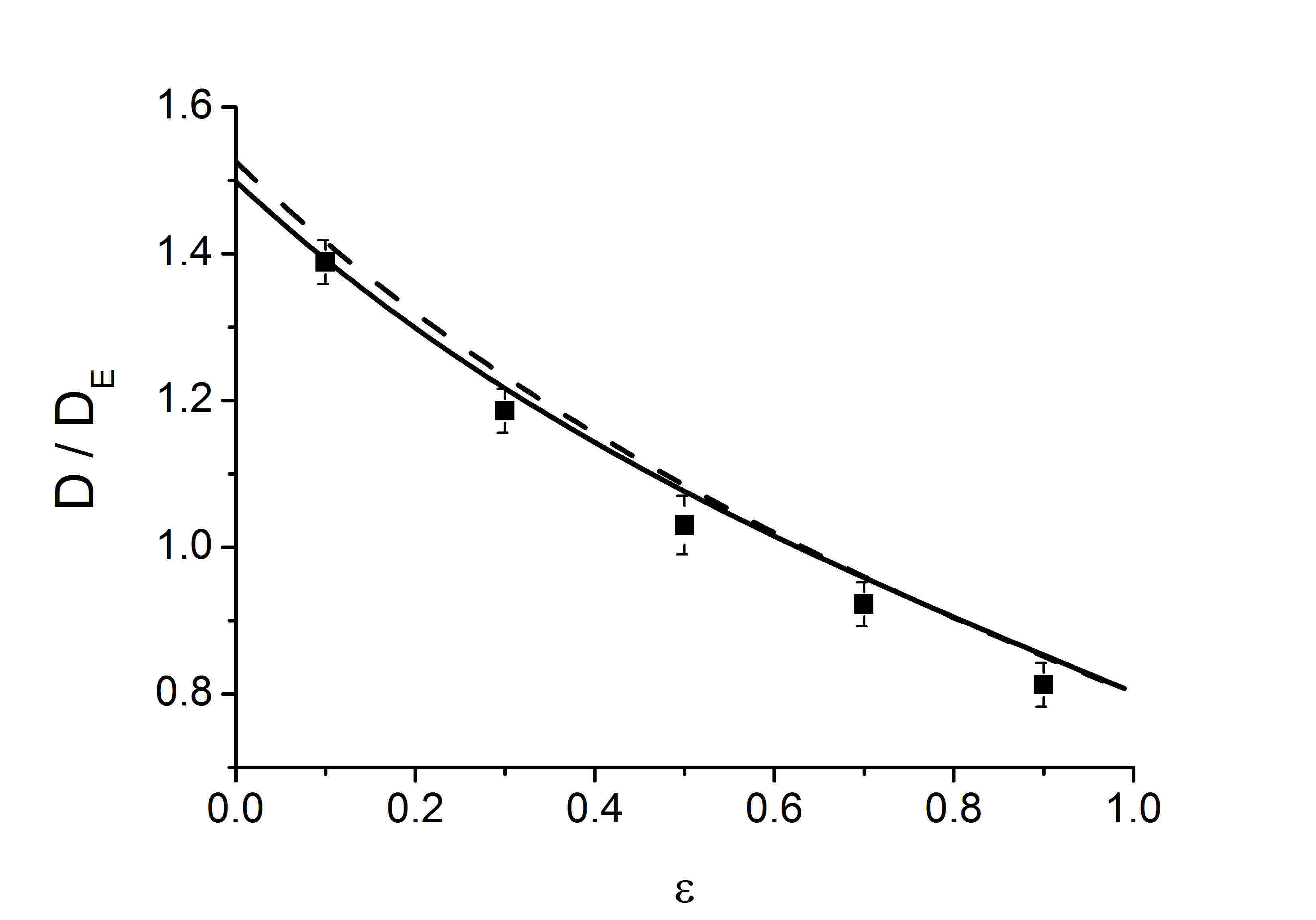
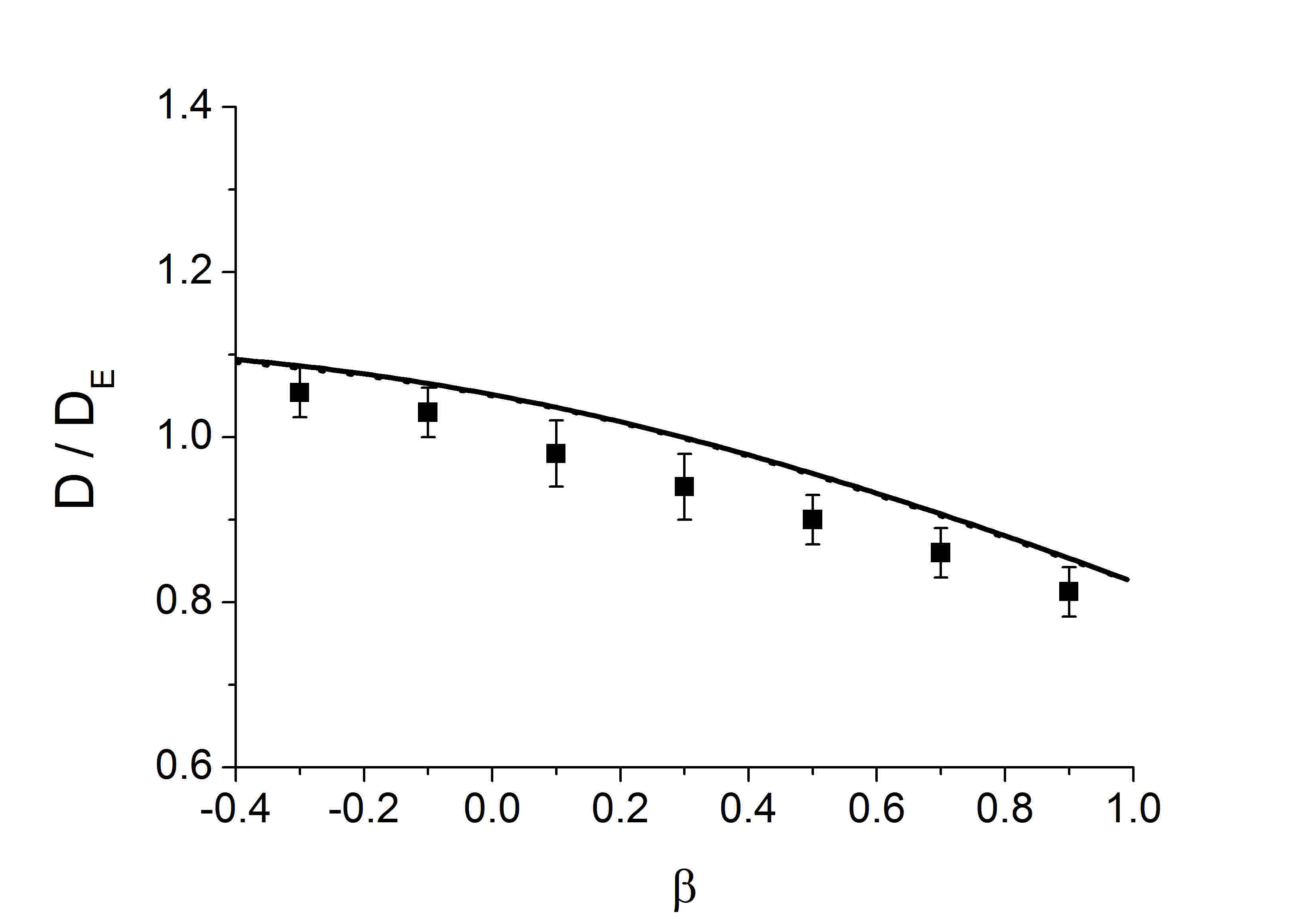
Figure 1: The dependence of the self-diffusion coefficient in a HCS on the normal $\varepsilon$ (upper panel) and tangential $\beta$ (lower panel) restitution coefficients. The MD simulation data (symbols) are compared with the predictions of the theory for a gas in a HCS, Eq. (31) (solid line) and Eq. (33) (dashed line, Maxwellian approximation). The fixed restitution coefficients are: $\beta=0.9$ for the upper and $\varepsilon=0.9$ for the lower panel.

As it may be seen from the figure, the relative diffusion coefficient $D(t)/D_{E}(t)$ increases with decreasing $\varepsilon$ – the dependence, which has been already observed for smooth particles [3, 4, 9, 5, 6, 2]. The physical nature of the effect is very simple: With the increasing inelasticity, which suppresses the normal component of the after-collisional relative velocity of particles, their trajectories become more stretched. This leads to the increasing correlation time and and hence, to a larger $D$. At the same time self-diffusion coefficient decreases for large roughness ($\beta>-0.25$) with increasing tangential restitution coefficient, see Fig. 1. It is not difficult to explain the observed behavior of $D$. Indeed, when the tangential restitution coefficient $\beta$ increases from $-1$ (smooth particles) to $+1$ (absolutely rough particles), the translational and rotational motion become more and more engaged [see Eqs. (2.1)] and the trajectories of particles more and more chaotic, that is, less stretched. This eventually causes the decrease of the diffusion coefficient with roughness.

As it is follows from the Fig. 1, the theoretical predictions for the self-diffusion coefficient are in a reasonably good agreement with the numerical data. The diffusion coefficient, calculated in the framework of the Maxwellian approximation, practically does not differ from the full solution, Eq. (33); the difference becomes apparent only for very high inelasticity ($\varepsilon<0.6$). A slight overestimate by the theory of the value of $D$, obtained in molecular dynamics, may be possibly attributed to the simple Ansatz (25) for the first-order function $f_{s}^{(1)}$, where only zero-order term of the expansion in the Sonine polynomials $S_{3/2}^{(k)}(v^{2}/v_{T}^{2})$ was used (see the footnote before Eq. (25)). One probably needs to extend the expansion and include the next order terms; this would be a subject of a future study.

4 Conclusion

We have analyzed an impact of particles’ roughness on the self-diffusion coefficient in granular gases. We use a simplified collision model with constant normal $\varepsilon$ and tangential $\beta$ restitution coefficients. The former characterizes the collisional dissipation of the normal relative motion of particles at a collision, the latter – of the tangential one. We develop an analytical theory for the self-diffusion coefficient, taking into account the deviation of the velocity-angular velocity distribution function from the Maxwellian; we use the leading-order terms in the expansion of this deviation in Sonine and Legendre polynomials series. We notice that the impact of the non-Maxwellian distribution on the self-diffusion coefficient is small. To check the predictions of our theory we perform the molecular dynamics simulations for a granular gas in a homogeneous cooling state for different values of the normal and tangential restitution coefficients. We find that the theoretical results are in a reasonably good agreement with the simulation data. Both the theory and molecular dynamics demonstrate that the relative diffusion coefficient $D(t)/D_{E}(t)$ ($D_{E}$ is the Enskog value of diffusion coefficient for smooth elastic particles) increases with decreasing normal restitution coefficient $\varepsilon$, similarly, as for a gas of smooth particles and decreases with increasing tangential restitution coefficient $\beta$ for large roughness ($\beta>-0.25$) .

References

- [1] Becker, V., Schwager, T., Poschel, T.: Coefficient of tangential restitution for the linear dashpot model. Phys. Rev. E 77, 011304 (2008); Schwager, T., Becker, V., Poschel, T.: Coefficient of tangential restitution for viscoelastic spheres. Eur. Phys. J. E 27, 107–114 (2008)
- [2] Bodrova, A.S., Brilliantov, N.V.: Granular gas of viscoelastic particles in a homogeneous cooling state. Physica A 388, 3315–3324 (2009)
- [3] Brey, J.J., Dufty, J.W., Santos, A.: Kinetic models for granular flow. J. Stat. Phys. 97, 281 (1999); Brey, J.J., Ruiz-Montero, M.J., Cubero, D., Garcia-Rojo, R.: Self-diffusion in freely evolving granular gases. Phys. Fluids 12, 876 (2000); Brey, J.J., Ruiz-Montero, M.J., Cubero, D., Garcia-Rojo, R.: Self-diffusion in freely evolving granular gases. Physics of Fluids 12(4), 876–883 (2000); Brey, J.J., Ruiz-Montero, M.J., Garcia-Rojo, R., Dufty, J.W.: Brownian motion in a granular gas. Phys. Rev. E 60, 7174 (1999)
- [4] Brilliantov, N.V., Pöschel, T.: Self-diffusion in granular gases. Phys. Rev. E 61(2), 1716–1721 (2000)
- [5] Brilliantov, N.V., Pöschel, T.: Kinetic theory of Granular Gases. Oxford University Press, Oxford (2004)
- [6] Brilliantov, N.V., Pöschel, T.: Self-diffusion in granular gases: Green-Kubo versus Chapman-Enskog. Chaos 15, 026108 (2005)
- [7] Brilliantov, N.V., Pöschel, T., Kranz, W.T., Zippelius, A.: Translations and rotations are correlated in granular gases. Phys. Rev. Lett. 98, 128001 (2007); Kranz, W.T., Brilliantov, N.V., Pöschel, T., Zippelius, A.: Correlation of spin and velocity in the homogenous cooling state of a granluar gas of rough particles. Eur. Phys. J. Special Topics 179, 91 – 111 (2009)
- [8] Chapman, S., Cowling, T.G.: The mathematical theory of Nonuniform gases. Cambridge University Press, Londom (1970)
- [9] Garz o, V.: Tracer diffusion in granular shear flows. Phys. Rev. E 66, 021308 (2002); Garz o, V., Montanero, J.M.: Diffusion of impurities in a granular gas. Phys. Rev. E 69, 021301 (2004)
- [10] Goldhirsch, I.: Rapid granular flows. Annu. Rev. Fluid Mech. 35, 267 (2003)
- [11] Goldhirsch, I., Noskowicz, S.H., Bar-Lev, O.: Nearly smooth granular gases. Phys. Rev. Lett. 95, 068002 (2005); Goldhirsch, I., Noskowicz, S.H., Bar-Lev, O.: Hydrodynamics of nearly smooth granular gases. J. Phys. Chem. 109, 21449–21470 (2005)
- [12] Luding, S., Huthmann, M., McNamara, S., Zippelius, A.: Homogeneous cooling of rough, dissipative particles: Theory and simulations. Phys. Rev. E 58, 3416–3425 (1998)
- [13] van Noije, T.P.C., Ernst, M.H.: Velocity distributions in homogeneous granular fluids: the free and the heated case. Granular Matter 1, 57–64 (1998)
- [14] Pöschel, T., Brilliantov, N.V.: Granular Gas Dynamics, Lecture Notes in Physics, vol. 624. Springer, Berlin (2003); Pöschel, T., Luding, S.: Granular Gases, Lecture Notes in Physics, vol. 564. Springer, Berlin (2001)
- [15] Pöschel, T., Schwager, T.: Computational Granular Dynamics. Springer, Berlin (2005)
- [16] Puglisi, A., Baldassarri, A., Loreto, V.: Fluctuation-dissipation relations in driven granular gases. Phys. Rev. E 66, 061305 (2002)
- [17] Saitoh, K., Bodrova, A., Hayakawa, H., Brilliantov, N.: Negative normal restitution coefficient found in simulation of nanocluster collisions. Phys. Rev. Lett. 105, 238001 (2010)
- [18] Santos, A., Kremer, G.M., dos Santos, M.: Sonine approximation for collisional moments of granular gases of inelastic rough spheres. Phys. Fluids 23, 030604 (2011)
- [19] Sarracino, A., Villamaina, D., Costantini, G., Puglisi, A.: Granular brownian motion. J. Stat. Mech.: Theory and Experiment P04013 (2010)
- [20] Walton, O.R.: Numerical simulation of inelastic frictional particle-particle interactions. In: M.C. Roco (ed.) Particle Two-Phase Flow, pp. 884–907. Butterworth, London (1993)
- [21] Zippelius, A.: Granular gases. Physica A 369, 143–158 (2006)