Simple Numerical Model of Laminated Glass Beams

Abstract

This contribution presents a simple Finite Element model aimed at efficient simulation of layered glass units. The adopted approach is based on considering independent kinematics of each layer, tied together via Lagrange multipliers. Validation and verification of the resulting model against independent data demonstrate its accuracy, showing its potential for generalization towards more complex problems.

url]http://mech.fsv.cvut.cz/ zemanj

1 Introduction

The most frequently used transparent material in the building envelopes is glass. It is a fragile material, which fails in a brittle manner. This is the reason for using safety glasses in a situation when there is a possibility of human impact or where the glass could fall if shattered.

Laminated glass is a multi-layer material produced by bonding two or more layers of glass together with a plastic interlayer, typically made of polyvinyl butyral (PVB). The interlayer keeps the layers of glass bonded even when broken, and its high strength prevents the glass from breaking up into large sharp pieces. This produces a characteristic ”spider web” cracking pattern when the impact is not powerful enough to completely pierce the glass. Multiple laminae and thicker glass decrease stress level, thereby increasing the load-carrying capacity of a structural member, too.

The focus of this study is on the establishing a simple and versatile framework for the analysis of mechanical behavior of laminated glass units. To keep the discussion compact, we restrict our attention to the linearly elastic response of layered glass beams in the small strain regime. The rest of the paper is organized as follows. Methods of analysis of laminated glass beams are introduced in Section 2, together with a brief characterization of the proposed numerical model. The principles of the method are described in detail in Sections 3 and 4. In particular, the mechanical formulation of the model is shown in Section 3. In the next section, the Finite Element discretization is presented. In Section 5, the proposed numerical technique is verified and validated against a reference analytical solution and publicly available experimental data. Finally, Section 6 concludes the paper and discusses future extensions of the method.

2 Brief overview of available methods

The most frequent approach to the analysis of glass structural elements was, for a long time, based on empirical knowledge. Such relations are sufficient for the design of traditional windows glasses. In modern architecture there has been a steadily growing demand on the use of transparent materials for large external walls and roof systems in the recent decades. Therefore, the detailed analysis of layered glass units is becoming increasingly important in order to ensure a reliable and efficient design.

In general, the complex behavior of laminated glass can be considered as an intermediate state of two limiting cases [1]. In the first case, the structure is treated as an assembly of two independent glass plates without any interlayer (the lower bound on stiffness and strength of a member), while in the second case, corresponding to the upper estimate of strength and stiffness, the glass unit is modeled as a monolithic glass (one glass plate with thickness equal to the total thickness of the glass plates). Both elementary cases, however, fail to correctly capture complex interaction among individual layers, leading to non-optimal layer thickness designs. Therefore, several alternative approaches to the analysis of layered glass structures have been proposed in the literature. These methods can be categorized into three basic groups:

• methods calibrated with respect to experimental measurements [2],

• analytical approaches [3, 4, 5],

• numerical models typically based on detailed Finite Element simulations [6, 7].

Applicability of analytical approaches to practical (usually large-scale) structures is far from being straightforward. In particular, the closed-form solution of the resulting equations is possible only for very specific boundary conditions and therefore have to be solved by an appropriate numerical method. Moreover, the analytical approaches are rather difficult to be generalized to beams with multiple layers. Therefore, it appears to be advantageous to directly formulate the problem in the discretized form, typically based on the Finite Element Method (FEM). Nevertheless, we would like to avoid fully resolved two- or three-dimensional simulations, cf. [6, 7], which lead to unnecessarily expensive calculations.

In this paper, we propose a simple FEM model inspired by a specific class of refined plate theories [8, 9, 10]. In this framework, each layer is treated as the Timoshenko beam with independent kinematics. Interaction between individual layers is captured by the Lagrange multipliers (with a physical meaning of shear stresses), which result from the conditions of inter-layer displacements compatibility. Such a refined approach circumvents the limitation of similar models available in typical commercial FEM systems, which employ a single set of kinematic variables and average the mechanical response through the thickness of the beam, e.g. [11]. Unlike the proposed approach, the averaging operation is too coarse to correctly represent the inter-layer interactions, see Section 5 for a concrete example.

3 Mechanical model of laminated beams

As illustrated in Figure 1, laminated glasses consist mostly of three layers. A local coordinate system is attached to each layer to allow for an efficient treatment of independent kinematics. In the following text, a quantity $a$ expressed in the local coordinate system associated with the $i$-th layer is denoted as $a^{(i)}$, whereas a variable without an index represents a globally defined quantity, cf. Figure 1.

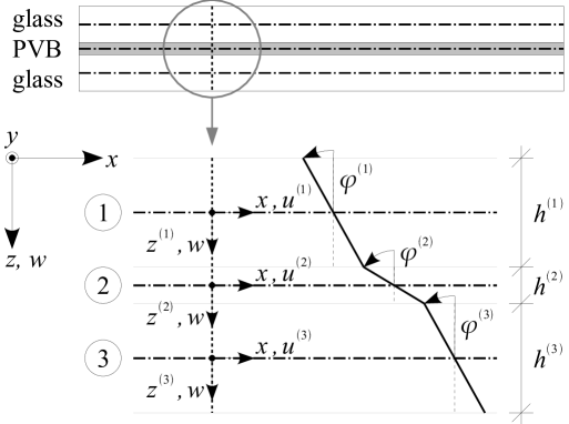
Figure 1: Kinematics of laminated beam

Each layer is modeled using the Timoshenko beam theory supplemented with membrane effects. Hence, the following kinematic assumptions are adopted

• the cross sections remain planar but not necessarily perpendicular to the deformed beam axis,

• vertical displacement does not vary along the height of the beam (when compared to the magnitude of the displacement).

Under these assumptions, the non-zero displacement components in each layer are parametrized as:

$$u^{(i)}(x,z^{(i)}) = u^{(i)}(x,0)+\varphi^{(i)}(x)z^{(i)},$$

$$w^{(i)}(x,z^{(i)}) = w(x),$$

where $i=1,2,3$ and $z^{(i)}$ is measured in the local coordinate system from the middle plane of the $i$-th layer. The inter-layer interaction is ensured via the continuity conditions specified on interfaces between layers in the form ($i=1,2$)

$$u^{(i)}(x,\frac{h^{(i)}}{2})-u^{(i+1)}(x,-\frac{h^{(i+1)}}{2})=0.$$ (1)

The strain field in the $i$-th layer follows from the strain-displacement relations [12, 11]

$$\varepsilon^{(i)}_{x}(x,z^{(i)}) = \mbox{$\displaystyle\frac{\partial{u^{(i)}}}{\partial{x}}$}(x,z^{(i)})=\mbox{$\displaystyle\frac{\,{\mathrm{d}}u^{(i)}}{\,{\mathrm{d}}x}$}(x,0)+\mbox{$\displaystyle\frac{\,{\mathrm{d}}\varphi^{(i)}}{\,{\mathrm{d}}x}$}(x)z^{(i)},$$

$$\gamma^{(i)}_{xz}(x) = \mbox{$\displaystyle\frac{\partial{u^{(i)}}}{\partial{z^{(i)}}}$}(x,z^{(i)})+\mbox{$\displaystyle\frac{\partial{w}}{\partial{x}}$}(x)=\varphi^{(i)}(x)+\mbox{$\displaystyle\frac{\,{\mathrm{d}}w}{\,{\mathrm{d}}x}$}(x),$$ (2)

which, when combined with the constitutive equations of each layer expressed in terms of Young’s modulus $E$ and the shear modulus $G$:

$$\sigma^{(i)}_{x}(x,z^{(i)})=E^{(i)}\varepsilon^{(i)}_{x}(x,z^{(i)}) \tau^{(i)}_{xz}(x)=G^{(i)}\gamma^{(i)}_{xz}(x),$$ and

yield the expressions for the internal forces as

$$N_{x}^{(i)}(x) = E^{(i)}A^{(i)}\mbox{$\displaystyle\frac{\,{\mathrm{d}}u^{(i)}}{\,{\mathrm{d}}x}$}(x,0),$$

$$V_{z}^{(i)}(x) = kG^{(i)}A^{(i)}\left(\varphi^{(i)}(x)+\mbox{$\displaystyle\frac{\,{\mathrm{d}}w}{\,{\mathrm{d}}x}$}(x)\right),$$

$$M_{y}^{(i)}(x) = E^{(i)}I^{(i)}\mbox{$\displaystyle\frac{\,{\mathrm{d}}\varphi^{(i)}}{\,{\mathrm{d}}x}$}(x),$$

where $b$ and $h^{(i)}$ are the width and height of the $i$-th layer, recall Figure 1, and $k=\frac{5}{6}$, $A^{(i)}=bh^{(i)}$ a $I^{(i)}=\frac{1}{12}b(h^{(i)})^{3}$ stand for the shear correction factor, the cross-section area and the moment of inertia of the $i$-th layer, respectively.

To proceed, consider the weak form of the governing equations, written for the $i$-th layer (the subscripts $\bullet_{x}$ and $\bullet_{z}$ related to internal forces and kinematics-related quantities are omitted in the sequel for the sake of brevity)

$$\int\limits_{0}^{L}\mbox{$\displaystyle\frac{\,{\mathrm{d}}missing}{\,{\mathrm{d}}x}$}\left(\delta u^{(i)}(x)\right)E^{(i)}A^{(i)}\mbox{$\displaystyle\frac{\,{\mathrm{d}}missing}{\,{\mathrm{d}}x}$}\left(u^{(i)}(x)\right)\,{\mathrm{d}}x=\int\limits_{0}^{L}\delta u^{(i)}(x)\bar{f}^{(i)}_{x}(x)\,{\mathrm{d}}x+\left[\delta u(x)\bar{N}^{(i)}(x)\right]_{0}^{L},$$

$$\int\limits_{0}^{L}\mbox{$\displaystyle\frac{\,{\mathrm{d}}missing}{\,{\mathrm{d}}x}$}\left(\delta w(x)\right)kG^{(i)}A^{(i)}\gamma^{(i)}(x)\,{\mathrm{d}}x=\int\limits_{0}^{L}\delta w(x)\bar{f}^{(i)}_{z}(x)\,{\mathrm{d}}x+\left[\delta w(x)\bar{V}^{(i)}(x)\right]_{0}^{L},$$

$$\int\limits_{0}^{L}\mbox{$\displaystyle\frac{\,{\mathrm{d}}missing}{\,{\mathrm{d}}x}$}\left(\delta\varphi^{(i)}(x)\right)E^{(i)}I^{(i)}\mbox{$\displaystyle\frac{\,{\mathrm{d}}missing}{\,{\mathrm{d}}x}$}\left(\varphi^{(i)}(x)\right)\,{\mathrm{d}}x=\left[\delta\varphi^{(i)}(x)\bar{M}^{(i)}(x)\right]_{0}^{L},$$

$$\int\limits_{0}^{L}\delta\gamma^{(i)}(x)kG^{(i)}A^{(i)}\left[\gamma^{(i)}(x)-\varphi^{(i)}(x)-\mbox{$\displaystyle\frac{\,{\mathrm{d}}missing}{\,{\mathrm{d}}x}$}\left(w(x)\right)\right]\,{\mathrm{d}}x=0.$$

to be satisfied for arbitrary admissible test fields $\delta u^{(i)}$, $\delta\varphi^{(i)}$ and $\delta w$. In particular, the first three equations correspond to equilibrium conditions written for normal and shear forces and bending moments, respectively. The last identity enforces the geometrical relation (2) in the integral form, thereby allowing to treat the shear strain as an independent field in the discretization procedure discussed next. Further note that the continuity conditions (1) will be introduced directly into the discretized formulation, as explained in the following Section.

4 Finite element discretization

To keep the discretization procedure transparent, it is assumed that each layer of the laminated beam is divided into identical number of elements, leading to the discretization scheme illustrated in Figure 2.

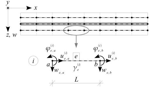
Figure 2: Finite element discretization of the $i$-th layer

Following the standard conforming Finite Element machinery, e.g. [12, 11], we express the searched and test displacement fields at the element level in the form

$$u^{(i)}_{e}(x)\approx\mathsf{N}^{(i)}_{e,u}(x)\mathsf{r}^{(i)}_{e,u}, \delta u^{(i)}_{e}(x)\approx\mathsf{N}^{(i)}_{e,u}(x)\delta\mathsf{r}^{(i)}_{e,u},$$

$$w_{e}(x)\approx\mathsf{N}_{e,w}(x)\mathsf{r}_{e,w}, \delta w_{e}(x)\approx\mathsf{N}_{e,w}(x)\delta\mathsf{r}_{e,w},$$

$$\varphi^{(i)}_{e}(x)\approx\mathsf{N}^{(i)}_{e,\varphi}(x)\mathsf{r}^{(i)}_{e,\varphi}, \delta\varphi^{(i)}_{e}(x)\approx\mathsf{N}^{(i)}_{e,\varphi}(x)\delta\mathsf{r}^{(i)}_{e,\varphi},$$

$$\gamma^{(i)}_{e}(x)\approx\mathsf{N}^{(i)}_{e,\gamma}(x)\mathsf{r}^{(i)}_{e,\gamma}, \delta\gamma^{(i)}_{e}(x)\approx\mathsf{N}^{(i)}_{e,\gamma}(x)\delta\mathsf{r}^{(i)}_{e,\gamma},$$

where $e$ is used to denote the element number, $\bullet_{e}$ and $\delta\bullet_{e}$ denote a relevant searched and test field restricted to the $e$-th element, $\mathsf{N}_{e,\bullet}^{(i)}$ is the associated matrix of basis functions and $\mathsf{r}^{(i)}_{e,\bullet}$ the matrix of nodal unknowns. In the actual implementation, the fields $u^{(i)}$, $w_{e}$ and $\varphi^{(i)}_{e}$, as well as the corresponding test quantities, are assumed to be piecewise linear. To obtain a locking-free element, the shear strain $\gamma^{(i)}_{e}$ is taken as constant and is eliminated using the static condensation, see [12, 11] for additional details.

To simplify the further treatment, we consider the following partitioning of the stiffness matrix $\mathsf{K}$ and the right hand side matrix $\mathsf{R}$ related to the $e$-th element and the $i$-th layer after the static condensation:

$$\left[\begin{array}[]{cc}\mathsf{K}^{(i)}_{e}&\mathsf{K}^{(i)}_{ew}\\ \mathsf{K}^{(i)}_{we}&\mathsf{K}^{(i)}_{w}\end{array}\right]\left[\begin{array}[]{c}\mathsf{r}^{(i)}_{e}\\ \mathsf{r}_{e,w}\end{array}\right]=\left[\begin{array}[]{c}\mathsf{R}^{(i)}_{e}\\ \mathsf{R}^{(i)}_{e,w}\end{array}\right],$$

where $\mathsf{K}^{(i)}_{ew}=\left(\mathsf{K}^{(i)}_{we}\right){\sf{}^{T}}$ and

$$\mathsf{r}^{(i)}_{e}=\left[u^{(i)}_{e,a},u^{(i)}_{e,b},\varphi^{(i)}_{e,a},\varphi^{(i)}_{e,b}\right]{\sf{}^{T}}, \mathsf{r}_{e,w}=\left[w_{e,a},w_{e,b}\right]{\sf{}^{T}}.$$

Considering all three layers in Figure 2 together gives the resulting system of governing equations in the form

$$\left[\begin{array}[]{ccccc}\mathsf{K}^{(1)}_{e}&\mathsf{0}&\mathsf{0}&\mathsf{K}^{(1)}_{ew}&\\ \mathsf{0}&\mathsf{K}^{(2)}_{e}&\mathsf{0}&\mathsf{K}^{(2)}_{ew}&\mathsf{E}_{e}{\sf{}^{T}}\\ \mathsf{0}&\mathsf{0}&\mathsf{K}^{(3)}_{e}&\mathsf{K}^{(3)}_{ew}&\\ \mathsf{K}^{(1)}_{we}&\mathsf{K}^{(2)}_{we}&\mathsf{K}^{(3)}_{we}&\mathsf{K}^{(1)}_{w}+\mathsf{K}^{(2)}_{w}+\mathsf{K}^{(3)}_{w}&\mathsf{0}\\ &\mathsf{E}_{e}&&\mathsf{0}&\mathsf{0}\end{array}\right]\left[\begin{array}[]{c}\mathsf{r}^{(1)}_{e}\\ \mathsf{r}^{(2)}_{e}\\ \mathsf{r}^{(3)}_{e}\\ \mathsf{r}_{e,w}\\ \mathsf{\lambda}_{(4\times 1)}\end{array}\right]=\left[\begin{array}[]{c}\mathsf{R}^{(1)}_{e}\\ \mathsf{R}^{(2)}_{e}\\ \mathsf{R}^{(3)}_{e}\\ \mathsf{R}^{(1)}_{e,w}+\mathsf{R}^{(2)}_{e,w}+\mathsf{R}^{(3)}_{e,w}\\ \mathsf{0}\end{array}\right],$$

where the matrix $\mathsf{\lambda}$ stores the nodal values of the Lagrange multipliers, associated with the compatibility constraint (1), and the matrix

$$\mathsf{E}_{e}=\left[\begin{array}[]{cccccccccccc}1&0&\frac{h^{(1)}}{2}&0&-1&0&\frac{h^{(2)}}{2}&0&0&0&0&0\\ 0&1&0&\frac{h^{(1)}}{2}&0&-1&0&\frac{h^{(2)}}{2}&0&0&0&0\\ 0&0&0&0&1&0&\frac{h^{(2)}}{2}&0&-1&0&\frac{h^{(3)}}{2}&0\\ 0&0&0&0&0&1&0&\frac{h^{(2)}}{2}&0&-1&0&\frac{h^{(3)}}{2}\end{array}\right]$$

implements the tying conditions.

5 Verification and validation of numerical model

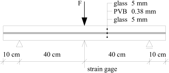
Figure 3: Three point bending setup for simply supported beam

To verify and validate the performance of the present approach, the previously described FEM model was implemented using MATLAB® system and compared against predictions of an analytical model and experimental data for a three-point bending test on a simply supported laminated glass beam presented in [5], see also Figure 3. The width of the beam is $b=0.1$ m and material data of individual components of the structure are available in Table 1. The glass modulus of elasticity is slightly lower than the conventional values of $70$–$73$ GPa reported in the literature and is specific for the material employed in the experiment. Moreover, as the PVB layer shows viscoelastic and temperature-dependent behavior, the modulus of elasticity corresponds to an effective secant value related to load duration of $60$ s and temperature of $22^{\circ}$ C.

Table 1: Material data

Glass PVB layer Young’s modulus, $E$ $64.5$ GPa $1.287$ MPa Poisson’s ratio, $\nu$ $0.23$ $0.4$

Table 2 summarizes values of the mid-span deflection for a representative load level determined by FE-based discretization using 60 elements (30 when symmetry of the problem is exploited) and the corresponding experimental values. Note that the discretization is sufficient to achieve three-digit accuracy in the mid-span deflection. In addition to the results obtained by an analytical method proposed by Asik and Tezcan in [5], the results of the analysis using ADINA® system and the elementary lower and upper bounds are included. In particular, the ADINA® model is based on the classical laminate theory, cf. [11], whereas the two simplified approaches assume zero or infinite compliance of the interlayer, recall also discussion in Section 2. In the following discussion, e.g. $\eta^{num}_{exp}$ denotes the relative error between the numerical prediction and reference experimental value, while e.g. $\eta_{an}$ is used for the error of analytical solution when compared to candidate approaches. Clearly, the results of the last three methods differ substantially from experimental data as well as the analytical results. The proposed numerical model, on the other hand, shows a response almost identical to the analytical method, which deviates from experimental measurement by less then $6\%$. Such accuracy can be considered as sufficient from the practical point of view.

Table 2: Comparison of results for a simply supported beam (load 50 N)

Model Central deflection [mm] $\eta_{exp}$ $\eta_{an}$ Laminated glass beam: thickness [mm] 5/0.38/5 (glass/PVB/glass) Experiment 1.27 - -5.2$\%$ Analytical model 1.34 5.5$\%$ - Numerical model 1.34 5.5$\%$ 0.0$\%$ ADINA ®(Multi-layered shell) 0.89 -30.2$\%$ -33.8$\%$ Monolithic glass beam: thickness [mm] 10 (glass+glass) Analytical model 0.99 -21.8$\%$ -25.9$\%$ Two independent glass beams: thickness [mm] 5/5 (without any interlayer) Analytical model 3.97 212.6$\%$ 196.2$\%$

To further confirm predictive capacities of the proposed numerical scheme, a response corresponding to a proportionally increasing load was investigated. The results appear in Tables 3 and 4. Again, the method seems to be sufficiently accurate in the investigated range of loads when considering the values of deflections as well as values of local stresses and strains.

Table 3: Comparison of deflections for a simply supported beam

Load [N] Central deflection [mm] $w_{exp}$ $w_{an}$ $\eta^{an}_{exp}$ [%] $w_{num}$ $\eta^{num}_{exp}$ [%] $\eta^{num}_{an}$ [%] 50 1.27 1.34 5.51 1.34 5.51 0.00 100 2.55 2.69 5.49 2.68 5.10 -0.37 150 4.12 4.03 -2.18 4.02 -2.43 -0.25 200 5.57 5.38 -3.41 5.36 -3.77 -0.37

Table 4: Comparison of stresses and strains for a simply supported beam

Load [N] Maximum strain [$\times 10^{-6}$] Maximum stress [MPa] $\epsilon_{an}$ $\epsilon_{num}$ $\eta^{num}_{an}$ [%] $\sigma_{an}$ $\sigma_{num}$ $\eta^{num}_{an}$ [%] 50 112 114 1.79 7.23 7.34 1.52 100 224 228 1.79 14.45 14.68 1.59 150 336 341 1.49 21.68 22.02 1.57 200 448 455 1.56 28.9 29.36 1.59

6 Conclusions

As shown by the presented results, the proposed numerical method is well-suited for the modeling of laminated glass beams, mainly because of its low computational cost and accurate representation of the structural member behavior. Future improvements of the model will consider large deflections and the time-dependent response of the interlayer and will be reported separately.

References

- [1] C. V. G. Vallabhan, J. E. Minor, S. R. Nagalla, Stress in layered glass units and monolithic glass plates, Journal of Structural Engineering 113 (1987) 36–43.
- [2] H. S. Norville, K. W. King, J. L. Swofford, Behavior and strength of laminated glass, Journal of Engineering Mechanics 124 (1998) 46–53.
- [3] C. V. G. Vallabhan, Y. C. Das, M. Magdi, M. Asik, J. R. Bailey, Analysis of laminated glass units, Journal of Structural Engineering 113 (1993) 1572–1585.
- [4] M. Z. Asik, Laminated glass plates: Revealing of nonlinear behavior, Computers and Structures 81 (2003) 2659–2671.
- [5] M. Z. Asik, S. Tezcan, A mathematical model for the behavior of laminated glass beams, Computers and Structures 83 (2005) 1742–1753.
- [6] A. V. Duser, A. Jagota, S. J. Bennison, Analysis of glass/polyvinyl butyral laminates subjected to uniform pressure, Journal of Engineering Mechanics 125 (1999) 435–442.
- [7] I. V. Ivanov, Analysis, modelling, and optimization of laminated glasses as plane beam, International Journal of Solids and Structures 43 (2006) 6887–6907.
- [8] S. T. Mau, A refined laminated plate theory, Journal of Applied Mechanics–Transactions of the ASME 40 (2) (1973) 606–607.
- [9] M. Šejnoha, Micromechanical modeling of unidirectional fibrous composite plies and laminates, Ph.D. thesis, Rensselaer Polytechnic Institute, Troy, NY (1996).
- [10] K. Matouš, M. Šejnoha, J. Šejnoha, Energy based optimization of layered beam structures, Acta Polytechnica 38 (2) (1998) 5–15.
- [11] K. J. Bathe, Finite Element Procedures, 2nd Edition, Prentice Hall, 1996.
- [12] Z. Bittnar, J. Šejnoha, Numerical methods in structural mechanics, ASCE Press and Thomas Telford, Ltd, New York and London, 1996.