CORS Baade-Wesselink distance to the LMC NGC 1866 blue populous cluster.

Abstract

We used Optical, Near Infrared photometry and radial velocity data for a sample of 11 Cepheids belonging to the young LMC blue populous cluster NGC 1866 to estimate their radii and distances on the basis of the CORS Baade-Wesselink method. This technique, based on an accurate calibration of the surface brightness as a function of (U-B), (V-K) colors, allows us to estimate, simultaneously, the linear radius and the angular diameter of Cepheid variables, and consequently to derive their distance. A rigorous error estimate on radius and distances was derived by using Monte Carlo simulations. Our analysis gives a distance modulus for NGC 1866 of 18.51$\pm$0.03 mag, which is in agreement with several independent results.

1 Introduction

One of the main goal of modern cosmology is the determination of the Hubble constant to an accuracy of 1-2% (Freedman et al., 2011, and references therein). The distance to the LMC is a critical step in the problem of determining the scale of the universe. It is, in fact, considered as a benchmark in the determination of distances to other galaxies, being a useful place to compare and test different distance estimators. Therefore, any error in its distance contributes a substantial fraction of the uncertainty in the Hubble constant (Mould et al., 2000).

In the last two decades there have been improvements in the determination of the LMC distance both theoretically (e.g. red clump, tip of red giant branch, model fitting of variable stars light curves; Romaniello et al., 2000; Walker et al., 2001; Keller & Wood, 2002; Bono, Castellani & Marconi, 2002; Marconi & Clementini, 2005; Keller & Wood, 2006; Grocholski et al., 2007; Koerwer, 2009), and observationally (e.g. parallaxes for Galactic Cepheids and RR Lyrae, eclipsing binaries; Popowski & Gould, 1998; Whitelock & Feast, 2000; Benedict et al., 2002; Fitzpatrick et al., 2002, 2003; Dall’Ora et al., 2004; Benedict et al., 2007, 2011; Bonanos et al., 2011). The literature contains a huge number of estimated distance values ranging from 18.10 mag (Udalski, 1998) to 18.80 mag (Groenewegen & Oudmaijer, 2000), a very unsatisfactory situation that indicates the presence of significant systematic errors in most of the methods. A summary of the results of different methods with the corresponding references can be found in Benedict et al. (2002, Tab.10).

Since the discovery by Leavitt (1908), the most used absolute calibration of the extragalactic distance scale is based on the Period–Luminosity relation of LMC Cepheids. Unfortunately, this procedure typically gives an indirect measure of the distance, because it calibrates the Period–Luminosity relation for LMC on the basis of the same relation obtained for Galactic Cepheids (see e.g. Persson et al., 2004). A strong drawback in this procedure is the role played by metallicity in the Period–Luminosity relation. From both the observational and theoretical perspective, some authors argue that this dependence is present (e.g. Freedman et al., 2001; Storm et al., 2003; Tammann Sandage & Reindl et al., 2003; Sakai et al., 2004; Romaniello et al., 2005; Macri et al., 2006; Freedman & Madore, 2011; Marconi, Musella & Fiorentino, 2005; Bono et al, 2008; Bono et al., 2010) , even if the size and the sign of the effect is still disputed, while others suggest that the effect is small and perhaps ill defined (e.g. Groenewegen & Salaris, 2003; Gieren et al., 2005; Storm et al., 2005, 2011b; Alibert et al., 1999).

In the Hubble Space Telescope H₀ Key Project by Freedman et al. (2001) a LMC distance modulus value of 18.50$\pm$0.10 mag has been adopted to calibrate several secondary distance indicators using the Cepheid variables. The adopted value of the LMC distance by Freedman and collaborators can be considered as a converging value for the LMC distance and as the watershed for the dichotomy between the so called ”short distance scale” (values lower than 18.50 mag) and the ”long distance scale” (values larger than 18.50 mag).

A direct measurement of the distance to the LMC can be obtained by using a version of the Baade–Wesselink technique called the surface brightness method (Gieren et al., 1997, and references therein). This method utilizes radial changes of the stellar surface brightness and the pulsational velocity for the determination of the linear radius and angular diameter of pulsating stars. Gieren et al. (2005) applied the near–infrared surface brightness technique to a sample of 13 Cepheids in the LMC and obtained a distance modulus of 18.56$\pm$0.04 mag. The same method has been applied recently by Storm et al. (2011b) who derived the distances of 36 Cepheids in the LMC and obtained a distance modulus of 18.45$\pm$0.04 mag.

In the present work we are going to face the problem of the LMC distance by means of the CORS version of the Baade-Wesselink surface brightness technique (Caccin et al., 1981; Ripepi et al., 1997, 2000; Ruoppo et al., 2004; Molinaro et al., 2011), using recent photometric and spectroscopic data of a sample of Cepheids observed in the populous cluster NGC 1866. This object is one of the few young ($\sim 10^{8}$ yr Brocato et al., 1989) LMC clusters that are close enough to allow the detailed observation of individual stars (see e.g. Mucciarelli et al., 2011; Brocato et al., 2003, and references therein). Moreover, Storm et al. (2005) found that the NGC 1866 Cepheids are close to the average LMC Cepheid distance, so we will assume the distance to this cluster to be the distance of the LMC itself. To date it is known that NGC 1866 harbors at least 23 Cepheids (Welch & Stetson, 1993; Musella et al., 2006), the largest number among all the LMC clusters, and this makes it an excellent system for distance determination. Indeed it provides a sizeable sample of variable stars contained in a limited volume and then all at the same distance. Furthermore, we expect they are characterized by the same chemical composition, age and reddening, so that we can derive their distance with no influence of differences in the above quantities among stars.

The first Baade–Wesselink distance to NGC 1866 was derived by Côté et al. (1991), obtaining the radii of seven variables in the field of NGC 1866 and using the B-V color to calibrate the surface brightness. The final result, 18.6$\pm$0.3 mag, is affected by a large error, probably due to the used color index, which is not a good surface brightness calibrator (Coulson Caldwell & Gieren, 1986).

Gieren, Richtler & Hilker (1994), using the surface brightness modification of the classical Baade–Wesselink method, obtained the distances of four Cepheids in the field of NGC 1866. They used the V-R color index and the radial velocities obtained from spectroscopic data taken at the Las Campanas 2.5 m du Pont reflector (Welch et al., 1991). The obtained distance modulus to NGC 1866 was 18.47$\pm$0.20 mag, considering only three Cepheids (HV 12198, HV 12199 and HV 12203). The fourth, HV 12204, was excluded because the authors suspected it was not a member of the cluster.

Finally, using optical and near–infrared data, Storm et al. (2005) derived the distance to NGC 1866 through the surface brightness method applied on five Cepheids and found 18.30$\pm$0.05 mag. We aim at improving their result by increasing the analyzed sample of Cepheids, thanks to new photometric and spectroscopic data, and by relying on an accurate calibration of the surface brightness obtained from grids of theoretical atmospheres.

Sec. 2 contains a description of the photometric and spectroscopic data used in this work. The procedures followed to phase the light curve the radial velocity curve and to correct for reddening are described in Sec. 3. The CORS Baade–Wesselink method is introduced in Sec. 4 together with the procedure adopted to calibrate the surface brightness function using atmosphere models. Sec. 5 contains the derived Cepheid angular diameter and the linear radii. The distance to NGC 1866 and the comparison with other results from the literature are discussed in Sec. 6 while conclusions are contained in Sec. 7.

2 The data

NGC 1866 harbors at least 23 Cepheids (Welch & Stetson, 1993; Musella et al., 2006). Among them we have selected those stars such that both near infrared and radial velocity data were available. The final sample consists of 11 Cepheids whose data are presented in the next two sections and are resumed in Tab. 2.

2.1 Photometry

We used photometric data in the ultraviolet U band, optical B, V, I bands and near infrared K band.

The U band data were obtained at Cerro Tololo Inter–American Observatory (CTIO) with 0.9 m, 1.5 m and 4.0 m telescopes.

The optical data were taken at VLT with FORS1 imager and consist in 69 images in B, 90 images in V and 62 images in I. Both ultraviolet and optical data were calibrated in the Johnson–Cousins photometric system. These VLT data have already been published in Musella et al. (2006). The complete UBVRI dataset used in this work, will be published in a forthcoming paper (Musella et al. in preparation), including a detailed discussion of the adopted procedure to reduce the data and to face the crowding problem.

As for the near infrared K band, we have used the dataset described in Storm et al. (2005) and Testa et al. (2007). Furthermore, we used unpublished data collected by J. Storm for the Cepheids V4, V7 and V8, which were calibrated using the data by Testa et al. (2007) as reference. The data from Testa et al. (2007) were calibrated in the LCO photometric system using the relations from Carpenter (2001). K band data from Storm et al. (2005) have been calibrated in the CIT photometric system.

To compare the photometric data with theoretical models (see Sec. 4.2) we have transformed the infrared data from CIT and LCO to SAAO photometric system through the simple transformation from Bessell & Brett (1988):

$$K_{SAAO}=K_{CIT}+0.014=K_{LCO}+0.014$$ (1)

where we have used also the relation $K_{CIT}=K_{LCO}$ from Storm et al. (2005).

2.2 Radial velocity

We used the radial velocity data from Storm et al. (2005), Storm et al. (2004) and Welch et al. (1991), obtained through the classical cross–correlation method. For three Cepheids, namely HV 12197, HV 12199 and We2, we used new data coming from the FLAMES VLT dataset by Mucciarelli et al. (2011, Appendix A). We note that our radial velocities are the first ones ever published for We2. The radial velocities for the quoted three Cepheids are listed in Tab. 1.

Table 1: The new radial velocities in Km/s for HV 12197, HV 12199 and We2 are listed in second, third and fouth columns respectively. The epochs of observations are in the first column.

Epoch (JD)	HV 12197	HV 12199	We2
53280.77407	312.8$\pm$0.8	320.3$\pm$1.0	276.1$\pm$ 1.2
53335.71398	287.8$\pm$0.7	314.8$\pm$1.1	285.6$\pm$ 1.0
53335.75731	289.8$\pm$1.1	315.0$\pm$0.8	285.0$\pm$ 1.0
53335.80046	289.8$\pm$0.6	316.8$\pm$0.9	282.6$\pm$ 0.9
53338.60509	283.0$\pm$0.7	319.8$\pm$0.9	302.2$\pm$ 1.0
53351.59229	293.5$\pm$1.0	316.9$\pm$1.0	286.4$\pm$ 1.1
53351.64296	293.4$\pm$1.1	318.1$\pm$1.2	286.3$\pm$ 0.8
53351.69311	294.1$\pm$0.9	319.4$\pm$1.0	288.1$\pm$ 0.9
53376.61793	290.8$\pm$0.8	282.1$\pm$0.8	301.4$\pm$ 1.0
53376.72984	292.7$\pm$1.0	284.4$\pm$0.9	302.9$\pm$ 0.8
53377.73544	312.7$\pm$1.1	311.7$\pm$1.0	321.4$\pm$ 0.9
53378.59190	298.1$\pm$0.8	312.3$\pm$1.0	282.1$\pm$ 0.8

The new radial velocity curves for HV 12197, HV 12199 and We2 are shown in Fig. 1 together with those from the other authors. The agreement between our data and the other samples is evident for HV 12197 and HV 12199, while a well–covered radial velocity curve is shown for We2. As for We2, we have also estimated the systematic velocity $V_{\gamma}$ obtaining 301.4 km/s with an accuracy $\sim$1 km/s, confirming its cluster membership.

Figure 1: The new radial velocity data for HV 12197, HV 12199 and We2 (filled circles) are shown together with those from Storm et al. (2005) (open triangles) and Welch et al. (1991) (open squares).

Finally we recall that from these spectroscopic data the iron content was also estimated following the approach described in Mucciarelli et al. (2011) (see also Appendix A). The [Fe/H] values for the three Cepheids are -0.39$\pm$0.05 dex for HV 12197, -0.38$\pm$0.06 dex for HV 12199 and -0.43$\pm$0.05 dex for We2. These values are fully consistent with the average iron content of the cluster [Fe/H]=-0.43$\pm$0.01 dex obtained from the analysis of a sample of static stars in NGC 1866 (Mucciarelli et al., 2011).

Table 2: The Cepheids considered in this work are listed in the first column, their period is in the second column and in the third column we list the source of the radial velocity data with the shift ($Km/s$), if any, in parentheses. Finally the epochs used to phase light curves and radial velocity curves are listed in the last column.

Star	Period (days)	Radial velocity references	Epochs (HJD)
HV 12197	3.143742	Storm et al. (2005), this work(-1.25), Welch et al. (1991)	2452998.5638
HV 12198	3.522805	Storm et al. (2004), Storm et al. (2005)(+2.8), Welch et al. (1991)(+1.1)	2452947.7500
HV 12199	2.639181	Storm et al. (2005), Welch et al. (1991), this work	2452993.6100
HV 12202	3.101207	Storm et al. (2005), Welch et al. (1991) a	2452930.8922
HV 12203	2.954104	Storm et al. (2005), Welch et al. (1991)	2452972.6731
V4	3.31808	Storm et al. (2005), Welch et al. (1991)	2452998.5651
V6	1.944252	Storm et al. (2005), Welch et al. (1991)	2452976.7400
V7	3.452075	Storm et al. (2005)(-3.4), Welch et al. (1991)	2452915.9000
V8	2.007157	Storm et al. (2005), Welch et al. (1991)	2452915.7700
We2	3.054847	this work	2452990.6712
We8	3.039855	Welch et al. (1991)	2452995.5394

^aThe shifts are the same as those described in Storm et al. (2005).

3 Data analysis

In this section we describe the steps performed to phase the light and the radial velocity curves, as well as to estimate the reddening in the direction of NGC 1866.

3.1 Construction of light curves and radial velocity curves

Cepheid photometric data were phased as usual, i.e. requiring that the maximum of light in B band occurs at phase zero, while the maximum in the other bands are shifted in phase as expected (Labhardt, Sandage & Tammann, 1997; Freedman, 1988, see e.g.). The adopted epochs and the periods are listed in Tab. 2. As the data were obtained at different times, to estimate the (V-K) and (U-B) colors, it was necessary to first interpolate each light curve at the same phase points. This was achieved by means of a C code, written by one of the authors, performing smoothing spline interpolation. A different procedure has been performed to interpolate the U band of HV 12197 and K band of We2 and We8. HV 12197 U band light curve, in fact, was poorly sampled, while the K band measurements for We2 and We8 were of lower quality with respect to the other variables. In these three cases we have performed the interpolation by using a template light curve. To construct the template we have calculated the mean ratios $A(K)/A(V)$ and $A(U)/A(V)$ of the light curve amplitudes in the K, U and V bands for all the stars of our sample showing well–covered light curves. Considering the V band light curve of the star to be interpolated, we have then calculated a ”normalized” template light curve characterized by zero mean magnitude and amplitude equal to one. Finally, the interpolation has been achieved by rescaling the template light curve, according to the estimated ratios, and shifting it to the mean magnitude of the investigated Cepheid.

To estimate the uncertainties of the interpolated magnitudes for all the Cepheids we have considered the rms of the residuals around the interpolated curve.

As for radial velocity curves, to obtain an accurate phasing with light curves, we have used the same epoch and period as for the photometry.

As cited in Sec. 2.2, for all the Cepheids, except We8, we have measurements from different data sets. To combine them, we corrected for possible shifts in radial velocity (see Tab. 2). They were determined by interpolating the most accurate sample of radial velocities and then by estimating the median distance – along the velocity axis – between the fitted curve and the other radial velocity samples.

3.2 Reddening determination

To correct the colors for extinction, we used the grids of models by Bessell et al. (1998) (http://wwwuser.oat.ts.astro.it/castelli/colors/bcp.html). They provided models with different metallicity values and we have linearly interpolated between solar ([Fe/H]=0.0 dex) and subsolar ([Fe/H]=-0.5 dex) metallicity grids to obtain models at the metallicity estimated by Mucciarelli et al. (2011) and equal to [Fe/H]=-0.43 dex.

In this step we followed the technique introduced by Dean et al. (1978) to derive the reddening of Cepheids. According to this method, the reddening is derived by shifting the observed points in a color–color diagram onto their intrinsic unreddened position, which can be obtained either using stars of known reddening or by using models. In particular, according to the models, the Cepheids occupy a narrow zone in the plane (V-I)–(B-V) (Fig. 2), which represents the unreddened locus (5000$\leq T_{e}\leq$6250, 1.0$\leq\log g\leq$4.0). Using this color–color plane, we plotted the point, whose coordinate are the mean observed colors of each Cepheid, and shifted it along the reddening vector, trying different values of E(B-V) and selecting all the values which make the star to lie on the grids. The mean of these values is an estimate of the E(B-V), and the width of the range of selected values can be assumed as the uncertainty on the mean value. The procedure is shown in Fig. 2 for the Cepheid V7 and the values of E(B-V) for all the other stars are listed in Tab. 3. We repeated the procedure using the unreddened locus defined by Dean et al. (1978) finding an excellent agreement.

Table 3: The values of reddening E(B-V) (second column) and their uncertainties (third column) for the selected Cepheids of NGC 1866 (first column).

Star	E(B-V)	$\delta$E(B-V)
HV 12197	–	–
HV 12198	0.102	0.018
HV 12199	0.082	0.018
HV 12202	0.03	0.02
HV 12203	0.02	0.02
V4	0.07	0.02
V6	0.05	0.02
V7	0.06	0.02
V8	0.091	0.009
We2	0.10	0.03
We8	0.06	0.02

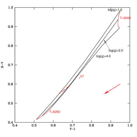
Figure 2: A schematic plot of the procedure followed to estimate the reddening E(B-V) from grids of theoretical models in the (B-V)–(V-I) plane. The locus expected to be occupied by Cepheids is enclosed between constant gravity and constant temperature curves (black and red lines respectively). As example, the representative point of the Cepheid V7 is out of the grids when it is not corrected for reddening. The values of E(B-V) which make the point to move along the reddening vector on the grids are selected (dashed line).

The procedure does not work for HV 12197 because its representative point is bluer than the grids along the V-I color. A possible explanation of this behavior can be the presence of a companion which can affect the color of the Cepheid expecially in optical bands (Szabados, 2003). In order to reduce the effect of outliers, we used the median of the derived reddening values obtaining E(B-V)=0.06 mag and a rms of 0.02 mag, consistent with the value typically adopted for NGC 1866 (see Storm et al., 2005, and references therein).

To calculate the extinction in each observational band, we used E(B-V)=0.06 mag, $R_{V}=3.3$ (Feast & Walker, 1987) and the law by Cardelli et al. (1989) obtaining $A_{U}=0.303$ mag, $A_{B}=0.261$ mag, $A_{V}=0.198$ mag, $A_{I}=0.120$ mag and $A_{K}=0.02$ mag.

4 The CORS Baade–Wesselink method

In the following sections, we give a brief description of the complete CORS Baade–Wesselink method used to derive the linear radius of Cepheid stars and of the procedure followed to calibrate the surface brightness function, which is at the base of the complete CORS technique. Moreover, the surface brightness allows us to estimate the star angular diameter and consequently the distance $d$ which is the factor linking the linear radius $R$ and the angular diameter $\theta$ according to $R=\frac{1}{2}d\theta$.

4.1 Theoretical background

The original CORS method (Caccin et al., 1981) is a realization of the classical Baade–Wesselink method (Wesselink, 1946) useful to derive the radius of pulsating stars.

Starting from the surface brightness function:

$$S_{V}=m_{V}+5\log\theta$$ (2)

where $\theta$ is the angular diameter (in mas) of the star and $m_{V}$ is the apparent visual magnitude, it is straightforward to obtain the basic CORS equation by differentiating with respect to the phase $(\phi)$, multiplying the result by a generic color index $(C_{ij})$ and integrating along the pulsational cycle:

$$q\int_{0}^{1}\!\ln\Big{\{}R_{0}-pP\int_{\phi_{0}}^{\phi}\!v(\phi^{\prime})d\phi^{\prime}\Big{\}}C^{\prime}_{ij}d\phi-B+\Delta B=0$$ (3)

where $q=\frac{5}{\ln 10}$, $P$ is the period, $v$ is the radial velocity and $p$ is the radial velocity projection factor, which correlates radial and pulsational velocities according to $R^{\prime}(\phi)=-p\cdot P\cdot v(\phi)$. The last two terms, $B$ and $\Delta B$, are:

$$B=\int_{0}^{1}C_{ij}(\phi)m^{\prime}_{V}(\phi)d\phi\hskip 10.0pt$$ (4)

$$\Delta B=\int_{0}^{1}C_{ij}(\phi)S^{\prime}_{V}(\phi)d\phi\;.$$ (5)

Equation (3) is an implicit equation in the unknown radius $R_{0}$ at an arbitrary phase $\phi_{0}$. The radius at any phase $\phi$ can be obtained by integrating the radial velocity curve. The main characteristic in the Eq.(3) is the estimate of the $\Delta B$ term as it contains the surface brightness function. Typically the $\Delta B$ term has a small value ($10^{-3}-10^{-4}$, Onnembo et al., 1985) and in the original Baade–Wesselink method it is neglected (see Caccin et al., 1981). However, the Cepheid radii estimated by including the $\Delta B$ term (complete CORS method) in the Eq.(3) are more accurate than those based on the original Baade–Wesselink method (Molinaro et al., 2011, and references therein).

4.2 The surface brightness calibration

To use the complete CORS technique, it is necessary to calibrate the surface brightness function. Here we describe only the main steps of the procedure followed and refer the reader to Molinaro et al. (2011) and references therein for more mathematical details.

Assuming the validity of the quasi–static approximation (Onnembo et al., 1985), for the Cepheid atmosphere, it is possible to express any photometric quantity as a function of effective temperature $T_{e}$ and gravity $\log g$. As a consequence, considering the surface brightness $S_{V}$ and two generic colors $C_{ij}$ and $C_{kl}$ they can be expressed as $S_{V}=S_{V}(T_{e},\log g)$ and $C_{ij}=C_{ij}(T_{e},\log g)$, $C_{kl}=C_{kl}(T_{e},\log g)$. If the last two equations can be inverted, it is possible to express effective temperature and gravity as function of the two colors and, consequently, the surface brightness becomes:

$$S_{V}=S_{V}(T_{e}(C_{ij},C_{kl}),\log g(C_{ij},C_{kl})).$$ (6)

In general, the invertibility condition is not valid over the entire parameter space, since the same pair of colors trace different pairs of gravity and temperature. However, after an appropriate choice of the colors $C_{ij}$ and $C_{kl}$ and of their range of variability, it is possible to find a local invertibility condition. Using grids of models provided by Bessell et al. (1998) (http://wwwuser.oat.ts.astro.it/castelli/colors/bcp.html) and interpolated at the correct metallicity values, we succeeded in inverting the previous equations for (U-B) and (V-K) colors and for the range of parameters typical of Cepheids with period $P\sim 3$ days: i.e. $0.5\leq\log g\leq 4.5$ dex and $5250\leq T_{e}\leq 6750$ K.

Figure 3 shows the selected region of the theoretical grids in the (V-K) (U-B) color–color plane containing the loops of all the analyzed Cepheids. For clarity reasons we show only data for a selected sample of objects. The loops outlined by HV12198 and HV12202 are representative of those drawn by the majority of Cepheids with the exception of We2 and HV12197. The loops of these two objects show extreme positions, with the bluest and the reddest (U-B) color respectively. This occurrence could be explained invoking the binarity of the target or, more likely, the presence of one or more blending objects. In this case, depending upon the angular separation between the Cepheid and the blended companions, relative to the radius of the seeing disk, it is possible to oversubtract or undersubtract the light of the companion. Similarly, the loop of HV12203 seems too extended (especially along the (U-B) direction) with respect to the average of “normal” Cepheids.

The effect of possible blending on the radius calculation has been analyzed in Sec. 5.2.

Within the plotted ranges of colors we have been able to fit the relations $\log T_{e}=\log T_{e}(V-K,U-B)$, $\log g=\log g(V-K,U-B)$ by means of polynomials. The fitted surfaces are shown in Figs. 4 and  5 and all the mathematical details are given in Appendix  B. The rms around the fitted relations amount to 0.00013 and 0.03 dex for $\log T_{e}$ and $\log g$ respectively.

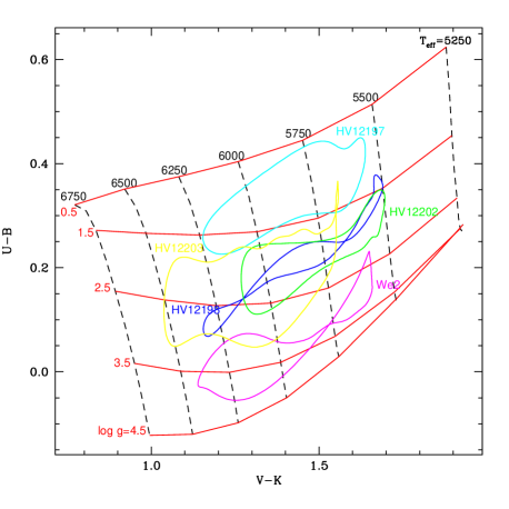
Figure 3: Color–color loops of five Cepheids of our sample plotted on the theoretical grids from Bessell et al. (1998). For clarity only a selected sample of objects is plotted (see text for details). Locus of constant temperature (dashed lines) and of constant gravity (continuous lines) are also plotted.

Figure 4: The surface representing $\log T_{e}$ as a function of (V-K) and (U-B) obtained from the fit of the atmosphere models (crosses) from Bessell et al. (1998).

Figure 5: The same as Fig. 4 but for $\log g$.

Using the fitted relations for temperature and gravity, we have derived the surface brightness from the following equation:

$$S_{V}=42.207-10.0\log T_{e}-BC$$ (7)

where the constant only depends on the bolometric absolute magnitude of the Sun, the solar constant and on the Stefan–Boltzmann constant (Fouqué & Gieren, 1997), while BC is the bolometric correction calculated as a function of the temperature and gravity through a polynomial fit (see Appendix  B). Figure  6 shows the fitted surface $BC=BC(\log T_{e},\log g)$ together with the models from Bessell et al. (1998).

Figure 6: The surface representing the bolometric correction $BC$ as a function of $\log T_{e}$ and $\log g$ obtained from the fit of the atmosphere models (crosses) from Bessell et al. (1998).

As a test of our calibration, we have analyzed the relation $F_{V}=F_{V}(V-K)$, where $F_{V}=4.2207-0.1S_{V}$ is the surface brightness parameter. Figure  7 shows the selected Cepheids plotted in the $F_{V}$–(V-K) plane together with the relation obtained by Kervella et al. (2004) using interferometric measurement of 9 Galactic Cepheids. The errors on the color (V-K) have been estimated by considering the scatter around the interpolated light curves, as explained in Sec. 3.1, while those on surface brightness have been estimated by means of simulations, as described in Appendix C below. The plot shows a small discrepancy between the fitted relation and the surface brightness of NGC 1866 Cepheids, which seems to be systematically brighter than the expected values from the relation by Kervella et al. (2004). Although the observed systematic shift is included within the uncertainty on reddening, it is important to stress that the relation by Kervella et al. (2004) has been obtained from Galactic Cepheids, which are more metal rich than those in NGC 1866. Therefore, the observed shift can be due to metallicity differences in the sense that less metallic Cepheids are more luminous than more metal rich ones. Then a metallicity dependence of the surface brightness relation is not ruled out.

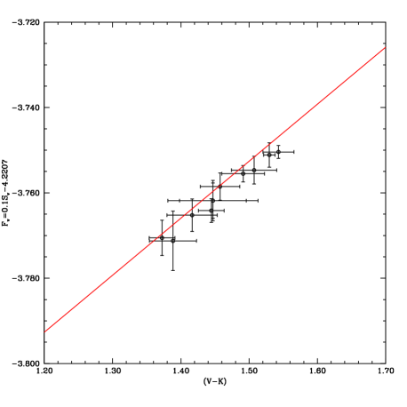
Figure 7: The selected Cepheids of NGC 1866 (black points) plotted in the plane $F_{V}$–(V-K) together with the surface brightness color relation obtained by Kervella et al. (2004) (solid line).

5 Derivation of the radius

This section contains the procedure followed to estimate the radii of the selected Cepheids and a comparison with other results present in the literature. Here we justify also the value of the projection factor $p$ chosen in our analysis.

5.1 The projection factor

One of the most uncertain parameter in the Baade–Wesselink method is the projection factor p, which converts the radial velocity into pulsational velocity. It depends both on physical structure of stellar atmosphere and the way the radial velocity is measured. Furthermore, there is an open discussion about its dependence on the period and/or pulsational phase. The question has been faced by many authors and the reader can find an exhaustive review in Barnes et al. (2009) and Storm et al. (2011a).

As mentioned before, the radial velocities used in this work have been derived with the cross–correlation method. In a recent work, Nardetto et al. (2009) achieved a period dependent value of the projection factor to correct radial velocity obtained by means of cross–correlation. Using their relation, namely $p=1.31-0.08\log p$, and the mean value of the period of our sample (once first-overtone are fundamentalized according to Feast & Catchpole, 1997), we calculated the projection factor value $p=1.27$. This is the same value found by Groenewegen (2007) by using Cepheids with interferometric angular diameters and HST parallaxes. Furthermore it allows us to be consistent with Molinaro et al. (2011), where they compare the two values $p=1.36$ and $p=1.27$ and found that the latter is the favoured one.

5.2 Radius calculation

Using the photometric data and the radial velocities discussed in Sec. 2, we are able to derive the mean radius for each star of our sample by using a FORTRAN 77 code. This performs a fit of the V magnitude curve, the (V-K), (U-B) color curves and the radial velocity curve using a Fourier fit, with a number of harmonics fixed interactively by the user. Then it solves the CORS Eq.  3 for the radius at an arbitrary phase both with and without the $\Delta B$ term. The mean radius is, finally, calculated by integrating the radial velocity curve twice. Our results are listed in Tab. 4. It contains the linear radii (in solar units) obtained from the CORS method and the angular diameters (in mas) calculated from the calibrated surface brightness Eq.(7), for the selected sample of Cepheids of NGC 1866 analysed in this work. The uncertainties on both the parameters are also listed and are obtained from Monte Carlo simulations as described in Appendix C. Note that for HV 12203 we provide only the radius obtained without the $\Delta B$ term (29.5$R_{\odot}$). Indeed, the inclusion of this term produces an anomalously small radius value (25.3$R_{\odot}$), as a consequence of the peculiar loop of HV12203 in the color–color plane (see Sec. 4.2) that, in turn, generates an unusually large value of the $\Delta B$ term ($\sim 10^{-2}$). The anomalous width of the HV 12203 loop has been considered in the estimate of the error on the angular diameter for this object.

Table  4 contains also the linear radii obtained by other authors for the stars in common with our sample. Their values have been rescaled to our projection factor value. Our results are systematically larger than those by Storm et al. (2005) and Gieren, Richtler & Hilker (1994), whereas they are consistent within the uncertainties with those by Côté et al. (1991), with the exception of HV 12199 which has a highly undetermined radius in his work.

Table 4: Mean linear radii (second column) and angular diameters (third column) of all selected Cepheids are listed with their uncertainties estimated from Monte Carlo simulations, as described in the text. The linear radii, expressed in solar units, listed in the remaining columns have been obtained by the following authors: Storm et al. (2005) (S05), Gieren, Richtler & Hilker (1994) (G94), Côté et al. (1991) (C91)

. Star     ($R\pm\delta R)(R_{\odot})$     ($\theta\pm\delta\theta$) ($\mu$-arcsec))     S05     G94     C91 HV 12197     31.6 $\pm$ 1.7 5.58 $\pm$ 0.08     23.9$\pm$0.6 – – HV 12198     33.1 $\pm$ 1.3 6.00 $\pm$ 0.06     27.5$\pm$0.4     28.3$\pm$2.6     38.3$\pm$6.3 HV 12199     27.9 $\pm$ 1.1 4.96 $\pm$ 0.08     23.0$\pm$1.0     24.6$\pm$3.1     56.1$\pm$19.1 HV 12202     29.6 $\pm$ 0.5 5.78 $\pm$ 0.08     26.3$\pm$0.9     –     25.2$\pm$4.4 HV 12203     29.5$\pm$ 0.7^a 5.22 $\pm$ 0.11     26.1$\pm$1.1     24.2$\pm$4.4     25.9$\pm$4.9 V4     30.2 $\pm$ 1.3 5.74 $\pm$ 0.04     –    –     29.3$\pm$8.1 V6     31.8 $\pm$ 1.3 5.10 $\pm$ 0.16     –    –     – V7     31.7 $\pm$ 2.0 5.92 $\pm$ 0.08     –    –     – V8     31.2 $\pm$ 2.3 5.18 $\pm$ 0.06     –    –     – We2     30.7 $\pm$ 1.1 5.68 $\pm$ 0.12     –    –     – We8     28.8 $\pm$ 1.0 5.40 $\pm$ 0.10     –    –     –

^aValue obtained without the $\Delta B$ term (see text).

As noted in Sec. 4.2 the color–color loops of We2 and HV12197 are systematically shifted in (U-B) with respect to the locus occupied by all other Cepheids on the grids of models in the (U-B), (V-K) plane. This could be due to the effect of overestimating or underestimating the flux in blue-ultraviolet bands, due to the difficult photometric analysis of crowded regions. To estimate the possible effect of blending on the derived radii, i.e. how the presence of a blue unresolved close companion affects the (U-B) color of the quoted Cepheids, we decided to shift along the (U-B) direction the two extreme loops described by We2 and HV12197, to match the region of the grids occupied by most of the Cepheids. This color shift is of the order of $\pm$0.08-0.09 mag. We then re-calculated the radii of these two Cepheids with the CORS method, obtaining as a result a difference in radii smaller than 1% and 4% for We2 and HV12197, respectively. Similarly, for the angular diameters the change was 0.3% and 0.5%, respectively. Therefore, our result is robust agaist the effect of contamination of the flux of Cepheids by undersubtracted or oversubtracted companions. This is due to the fact that blending affects only the value of the $\Delta B$ term, which typically has a small value (see Sec. 4.1) and influences the radius at most by about 5$\%$ on average (see Molinaro et al., 2011, and references therein). In any case, we will take into account this possible source of systematic uncertainty, by adding it to the random errors on the radius and surface brightness (obtained as in Appendix C).

Using the results of our procedure, we investigated how the selected Cepheids locate with respect to the Galactic period–radius relation recently obtained by Molinaro et al. (2011). A visual comparison is shown in Fig. 8 and it is evident that the Cepheids in NGC 1866 lie on the same period–radius relation as Galactic Cepheids. As a test we have fitted the equation $\log R=a+b\log P$ to the sample including the 26 Galactic Cepheids by Molinaro et al. (2011) and the stars analyzed in the present work, with exception of the first overtone pulsators (V6 and V8). The fitting relations are the following:

$$\log R=(1.120\pm 0.019)+(0.723\pm 0.019)\log P$$ (8)

$$\log R=(1.110\pm 0.015)+(0.746\pm 0.015)\log P$$ (9)

respectively excluding and including the $\Delta B$ term. The inclusion of the Cepheids belonging to NGC 1866 extends the Period–Radius relation in the direction of short periods, giving stronger constraints on the coefficients of the fit. It is important to stress that the equation in the case with the $\Delta B$ term remains almost unchanged with respect to that found by Molinaro et al. (2011), but with smaller uncertainties on the coefficients of the period–radius relation. Concerning the case without $\Delta B$ term, the fitting equation is slightly different with respect to that by Molinaro et al. (2011), but in any case consistent within the uncertainties.

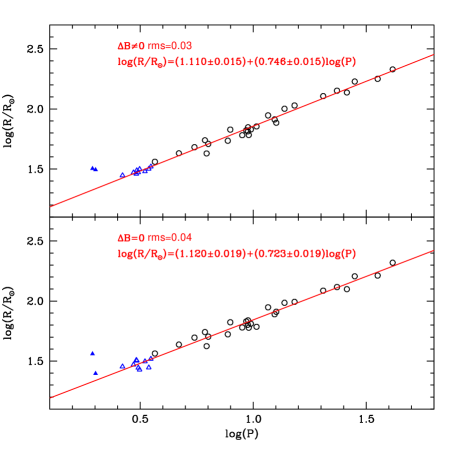
Figure 8: Period–radius relation obtained by combining the sample of 26 Galactic Cepheids by Molinaro et al. (2011) (empty circles) with those selected in the present work (empty triangles). The two panels refers to the fit including the term $\Delta B$ (upper panel) and excluding it (bottom panel). The fitting equations and the scatter around the fit are also indicated. The first overtone pulsators (filled triangles) are excluded from the fit.

6 Distance to NGC 1866

Using the values of the angular diameter, derived from the surface brightness, and the CORS Baade–Wesselink linear radius we have estimated the distance to NGC 1866 by using the simple equation $d(kpc)=2R(UA)/\theta(mas)$, where R and $\theta$ are the mean linear radius and angular diameter respectively.

The typical procedure used in other works (Fouqué & Gieren, 1997; Storm et al., 2005, 2011a), consisting in matching the curves of linear radius and angular diameter, gives the same result. In particular, we have performed a correction for eventual phase shift between the two curves and then the distance is calculated as the parameter that minimizes the quantity $\sum(R(\phi_{i})-\frac{d}{2}\theta(\phi_{i}))^{2}$, where the index i runs over the phases from 0.0 to 0.8. The phase cut has been performed to avoid the influence from possible shocks in the stellar atmosphere close to the minimum radius (see e.g. Storm et al., 2004).

As an example of radial curve matching, we report the case of We 2. In particular, Fig. 9 shows the linear radius of We 2 as a function of the phase and the curve of angular diameter corrected for phase shift and multiplied for the best distance value obtained from the minimization of the function cited above. It is evident from the plot that the two curves deviate at phases larger than 0.8, which have been excluded in the matching procedure.

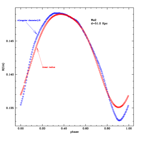
Figure 9: Example of matching between linear radius curve and angular diameter curve for the Cepheid We 2.

The distances in kpc of the Cepheids analyzed in the present work are listed in Tab. 5. The corresponding distance moduli, $\mu=m-M=-5+5\log[d(pc)]$, are also reported in the same table and are plotted in Fig. 10 as a function of the period.

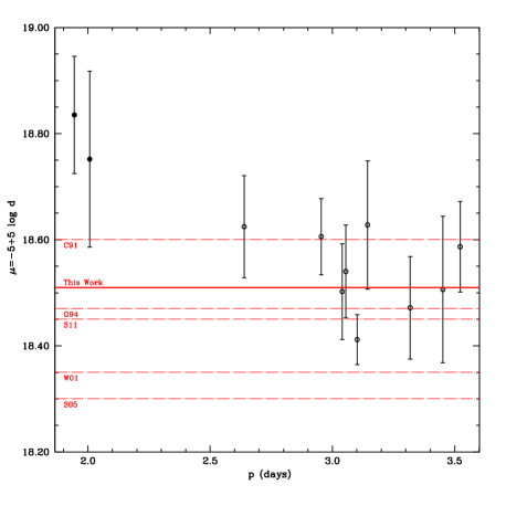
Figure 10: Distance moduli ($\mu$), with error–bars, of fundamental Cepheids (empty circles) and first overtones (full points) are plotted as function of the period (P) expressed in days. Our best distance estimate (solid line) is plotted together with the results by other authors (point–dashed lines): Storm et al. (2011b), Storm et al. (2005) (S05), Walker et al. (2001) (W01), Gieren, Richtler & Hilker (1994) (G94), Côté et al. (1991) (C91).

In our analysis we exclude the two overtone pulsators, whose distances are clearly discrepant (apparently more distant at a 3$\sigma$ level) with respect to the other considered stars (see Fig. 10). Since the Cepheids in NGC 1866 are expected to be all nearly at the same distance, this occurrence could be due to an imperfect calibration of the surface brightness function of overtones throughout the grids of model atmosphere. Further analysis is required about this point.

Using a weighted statistic of the 9 remaining Cepheids, we obtain a distance of 50.3$\pm$0.6 kpc corresponding to 18.51$\pm$0.03 mag in distance modulus and a rms of 0.09 mag. However, if we do not consider the weight, the mean distance becomes 51.1$\pm$0.6 kpc, equal to a distance modulus $\mu=$18.54$\pm$0.03 mag with rms of 0.07 mag. Since we are confident that our estimate of errors for each single Cepheid are correct, we consider the weighted result as our best value for the distance to NGC 1866.

The distance obtained in this work is 0.21 mag larger than that obtained by Storm et al. (2005), but it is consistent with their recent result 18.45$\pm$0.04 mag, obtained by calibrating the Period–Luminosity relation from the infrared surface brightness technique, although they used a different value of the projection factor (Storm et al., 2011b). The distance to NGC 1866 has been also derived by using other methods. As an example, Walker et al. (2001) used Hubble Space Telescope V and I photometry of stars in NGC 1866 to apply the Main Sequence fitting technique, obtaining a distance equal to 18.35$\pm$0.05 mag, which is shorter than our result. On the contrary, in a recent work Salaris et al. (2003) obtained the distance to NGC 1866 from the Red Clump technique. Their analysis gave a distance modulus of 18.53$\pm$0.07 mag, in agreement with our result.

Table 5: The distances of the selected Cepheids expressed in kpc (second column) and their distance modulus (third column) obtained from the CORS Baade–Wesselink linear radius and the angular diameters derived by the surface brightness.

Star	($d\pm\delta d)(kpc)$	Distance modulus (mag)
HV 12197	53.2 $\pm$ 3.0	18.63$\pm$0.12
HV 12198	52.2 $\pm$ 2.0	18.59$\pm$0.08
HV 12199	53.1 $\pm$ 2.3	18.62$\pm$0.10
HV 12202	48.1 $\pm$ 1.0	18.41$\pm$0.05
HV 12203	52.6 $\pm$ 1.7	18.61$\pm$0.07
V4	49.5 $\pm$ 2.2	18.47$\pm$0.10
V6	58.5 $\pm$ 2.9	18.83$\pm$0.11
V7	50.3 $\pm$ 3.2	18.51$\pm$0.14
V8	56.3 $\pm$ 4.2	18.75$\pm$0.17
We2	51.0 $\pm$ 2.0	18.54$\pm$0.09
We8	50.2 $\pm$ 2.1	18.50$\pm$0.09

7 Conclusions

In this work we derived the distance to the LMC young populous cluster NGC 1866. To this aim, we applied the CORS Baade–Wesselink technique (Caccin et al., 1981; Ripepi et al., 1997, 2000; Ruoppo et al., 2004; Molinaro et al., 2011) to a sample of 11 Cepheids belonging to the cluster. This method allows to obtain the linear radius through the combination of photometric and spectroscopic data and the angular diameter from the calibration of the surface brightness function by means of grids of model atmosphere. Finally, the distance is easily obtained by combining both linear and angular diameter in the equation $d(kpc)=2R(UA)/\theta(mas)$. Our work extends the sample of Cepheids studied by Storm et al. (2005) thanks to new photometric and spectroscopic data.

We obtained the reddening correction by applying the technique introduced by Dean et al. (1978) in the (V-I)–(B-V) color–color plane and obtained the value E(B-V)=0.06$\pm$0.02 mag, which coincides with the standard value used for NGC 1866 (see Storm et al., 2005, and references therein).

As for the projection factor, we used the appropriate value p=1.27, obtained from a recent p-factor–$\log P$ relation introduced by Nardetto et al. (2009) and already adopted in Molinaro et al. (2011)

The linear radii obtained from the CORS technique result to be larger than those derived by Gieren, Richtler & Hilker (1994) and Storm et al. (2005) for some stars of our sample. On the contrary, we are in good agreement with the results obtained by Côté et al. (1991).

We studied also how the selected Cepheids place with respect to the Period–Radius relation obtained by Molinaro et al. (2011) for Galactic Cepheids. Our analysis shows that the Cepheids in NGC 1866 follow the same linear relation than the Galactic ones.

A weighted statistical analysis gives a distance modulus of NGC 1866 equal to 18.51$\pm$0.03 mag and a rms of 0.09 mag.

Finally, the distance obtained in this work is in agreement with the converging value of 18.50 mag for LMC obtained by many authors and described in the introduction.

Appendix A Spectroscopic data

The new spectroscopic measurements for the three Cepheids HV 12197, HV 12199 and We2, were secured with FLAMES VLT under the program 074.D-0305. The observations were performed in the GIRAFFE mode and employing three different setups, namely HR 11 (with a coverage between 5597 and 5840 $\mathring{A}$), HR 12 (5821–6146 $\mathring{A}$) and HR 13 (6126–6405 $\mathring{A}$), with spectral resolutions ranging from 19000 and 24000. Five exposures were secured for HR 11, four for HR 12 and three for HR 13 (all the exposures are of 3600 s each).

Each exposure was analyzed independently. The spectra were reduced using the girBLDRS pipeline developed at the Geneva Observatory including bias subtraction, flat–fielding, wavelength calibration with a reference Th–Ar lamp and the final extraction of each spectrum. The accuracy of the zero–point in the wavelength calibration was checked by measuring the position of some sky–emission lines, compared with their rest–frame position taken from the sky–emission lines atlas by Osterbrock et al. (1996). No relevant shift was detected in the emission lines position, confirming the reliability of the adopted wavelength solution.

The girBLDRS pipeline performs, in its last step, the measurement of the radial velocity through the classical cross–correlation technique (Tonry & Davis, 1979). Heliocentric corrections were applied to each radial velocity. The typical uncertainty in the derived velocity of each exposure is of about 0.8 km/s.

The measurement of the iron content of the three cepheids was performed following the same approach already employed in the Mucciarelli et al. (2011) concerning the chemical analysis of a sample of stars in NGC1866. In each spectrum we identify a number of reliable, unblended iron lines (typically 10-15 in each spectrum), deriving their abundance through the $\chi^{2}$-minimization of the observed line profile with a grid of synthetic spectra computed with different Fe abundances. The computation of the synthetic spectra were performed by means the SYNTHE code (Kurucz, 1993) coupled with the ATLAS9 model atmospheres.

Appendix B The fit of theoretical grids.

Here we give the explicit mathematical expression of the surfaces obtained by interpolating $\log T_{e}$ and $\log g$ as a function of the two colors (U-B) and (V-K), and that describing the bolometric correction BC as a function of $\log T_{e}$ and $\log g$:

$$\log T_{e}=a_{1}+a_{2}(V-K)+a_{3}(V-K)^{2}+a_{4}(V-K)(U-B)+$$ (B1)

$$+a_{5}(V-K)^{2}(U-B)+a_{6}(V-K)(U-B)^{2}+$$

$$a_{7}(U-B)^{3}+a_{8}(V-K)^{3}+a_{9}(U-B)^{2}+a_{10}(U-B)$$

$$\log g=b_{1}+b_{2}(V-K)^{2}+b_{3}(V-K)(U-B)+b_{4}(V-K)^{2}(U-B)+$$ (B2)

$$+b_{5}(V-K)(U-B)^{2}+b_{6}(U-B)^{3}+b_{7}(V-K)^{3}+b_{8}(U-B)^{2}+b_{9}(U-B)$$

$$BC=c_{1}+c_{2}\log T_{e}+c_{3}(\log T_{e})^{2}+c_{4}(\log T_{e})(\log g)+c_{5}(\log T_{e})^{2}(\log g)+$$ (B3)

$$+c_{6}(\log T_{e})(\log g)^{2}+c_{7}(\log g)^{3}+c_{8}(\log g)^{2}+c_{9}\log g$$ (B4)

The coefficients $a_{i},\,b_{i},\,c_{i}$ of the previous equations are listed in Tab. 6. The rms of the previous relations are 0.00013 dex, 0.0007 dex and 0.0012 respectively.

Table 6: Coefficients of the polynomial equations obtained from the interpolation of temperature, gravity and bolometric correction.

$a_{1}$	$a_{2}$	$a_{3}$	$a_{4}$	$a_{5}$	$a_{6}$	$a_{7}$	$a_{8}$	$a_{9}$	$a_{10}$
3.9858$\pm$0.0019	-0.208$\pm$0.005	0.055$\pm$0.004	0.110$\pm$0.008	-0.031$\pm$0.004	0.057$\pm$0.008	-0.029$\pm$0.007	-0.0093$\pm$0.0011	-0.071$\pm$0.007	-0.121$\pm$0.004
$b_{1}$	$b_{2}$	$b_{3}$	$b_{4}$	$b_{5}$	$b_{6}$	$b_{7}$	$b_{8}$	$b_{9}$	$b_{10}$
5.51$\pm$0.09	-4.61$\pm$0.18	25.9$\pm$1.6	-14.0$\pm$0.8	24.5$\pm$1.5	-13.2$\pm$1.3	2.65$\pm$0.10	-21.7$\pm$1.4	-19.4$\pm$0.8
$c_{1}$	$c_{2}$	$c_{3}$	$c_{4}$	$c_{5}$	$c_{6}$	$c_{7}$	$c_{8}$	$c_{9}$	$c_{10}$
-221.0$\pm$7.4	114.9$\pm$4.0	-14.9$\pm$0.5	-21.4$\pm$1.8	2.9$\pm$0.2	-0.106$\pm$0.009	0.00160$\pm$0.00016	0.39$\pm$0.03	40.2$\pm$3.4

Appendix C Error estimate on radii through Monte Carlo simulations

To investigate how the errors in the various parameters, involved in the CORS method, influence the linear radius estimation, we have performed Monte Carlo simulations. In particular we have considered the uncertainties on the colors (V-K) and (U-B), on the reddening E(B-V) and the error in the phase matching between the photometric and radial velocity curves. We have run 1000 simulations for each of the cited parameters. They consist in varying each analyzed parameter using random numbers extracted from a Gaussian distribution with an rms equal to the error on the parameter itself. For all the extracted displacements the radius is recalculated and the rms of the obtained values is assumed as the uncertainty in the radius due to the error on the analyzed parameter. As for the colors (V-K) and (U-B) we have derived their errors from the scatter around the interpolated light curves. Here we do not give all the derived errors in the colors, but remind only that typical values are $\sim$0.03 mag for both the (V-K) and (U-B), except for few cases with errors of $\sim$0.06 mag because of less sampled light curve in the K and/or U bands. For the three Cepheids HV12197, HV12203, and We2, an additional systematic error has been considered for the (U-B) color, leading to a total uncertainty of the order of 0.085-0.10 mag. The effect of the reddening on the radius estimation has been analyzed by considering the error of 0.02 mag obtained as described in Sec. 3, while for the phase matching we have chosen a typical error of 0.01 in phase. This value has been chosen to be conservative, because the error on the phase matching, due to the uncertainty on the period propagated between the epoch of photometry and that of spectroscopy, is typically smaller. Furthermore, we have taken into account the fact that the star HV 12202 is a spectroscopic binary (Welch et al., 1991) and consequently its photometry and radial velocity can be influenced by the flux and the motion of the companion respectively. To be conservative we have doubled the errors on the photometry and the radial velocity data. The total effect of the various errors on the radius is always less than 5$\%$, with exception of V7 and V8 for which it is $\sim$7$\%$ (Tab. 4).

Monte Carlo simulations have been used also to estimate the errors on the surface brightness. As it depends on the two colors (V-K) and (U-B) through the equations given in Appendix B, we have run 1000 simulations for each color following the same procedure described before. The derived error on the surface brightness has been used to calculate the uncertainty on the angular diameter, obtained from the Eq.(7) and reported in Tab. 4.

References

- Alibert et al. (1999) Alibert, Y., Baraffe, I., Hauschildt, P. & Allard, F., 1999, A&A, 344, 551
- Barnes et al. (2009) Barnes T. G., III, 2009, in Guzik J. A., Bradley P. A., eds, AIP Conf. Proc. Vol. 1170, Stellar Pulsation: Challenges for Theory and Observation. Am. Inst. Phys., New York, p. 3
- Benedict et al. (2002) Benedict, F.G., et al., 2002, AJ, 123, 473
- Benedict et al. (2007) Benedict, F.G., et al., 2007, AJ, 133, 1810
- Benedict et al. (2011) Benedict, G.F., McArthur, B.E., Feast, M.W., et al., 2011, arXiv:1109.5631
- Bessell & Brett (1988) Bessell, M.S. & Brett, J.M., 1988, PASP, 100, 1134
- Bessell et al. (1998) Bessell, M.S., Castelli F. & Plez, B., 1998, A&A, 333, 231
- Bonanos et al. (2011) Bonanos, A.Z., Castro, N., Macri, L.M. & Kudritzki, R.P., 2011, ApJ, 729, 9
- Bono, Castellani & Marconi (2002) Bono, G., Castellani, V. & Marconi, M., 2002, ApJ, 565, L83
- Bono et al (2008) Bono, G., Caputo, F., Fiorentino, G., Marconi, M. & Musella, I., 2008, ApJ, 684, 102
- Bono et al. (2010) Bono, G., Caputo, F., Marconi, M. & Musella, I., 2010, ApJ, 715, 277
- Brocato et al. (1989) Brocato, E., Buonanno, R., Castellani, V. & Walker, A.R., 1989, ApJS, 71, 25
- Brocato et al. (2003) Brocato, E., Castellani, V., Di Carlo, E., Raimondo, G. & Walker, A.R., 2003, AJ, 125, 3111
- Caccin et al. (1981) Caccin, R., Onnembo, A., Russo, G., Sollazzo, C., 1981, A&A, 97, 104
- Cardelli et al. (1989) Cardelli, J.A., Clayton, G.C. & Mathis, J.S., 1989, AJ, 345, 245
- Carpenter (2001) Carpenter, J.M., 2001, AJ, 121, 2851
- Côté et al. (1991) Côté, P., Welch, D.L., Mateo, M., Fischer, P. & Madore, B., 1991, AJ, 101, 5
- Coulson Caldwell & Gieren (1986) Coulson, I.M., Caldwell, J.A.R. & Gieren, W.P., 1986, ApJ, 303, 273
- Dall’Ora et al. (2004) Dall’Ora, M., et al., 2004, AJ, 610, 269
- Dean et al. (1978) Dean, J.F., Warren, P.R. & Cousins, A.W.J., 1978, MNRAS, 183, 569
- Feast & Walker (1987) Feast, M.W. & Walker, A.R., 1987, ARA&A, 25, 345
- Feast & Catchpole (1997) Feast, M.W. & , Catchpole, R.M., 1997, MNRAS, 286, L1
- Fitzpatrick et al. (2002) Fitzpatrick, E.L., Ribas, I., Guinan, E.F., DeWarf, L.E., Maloney, F.P. & Massa, D., 2002, ApJ, 564, 260
- Fitzpatrick et al. (2003) Fitzpatrick, E.L., Ribas, I., Guinan, E.F., Maloney, F.P. & Claret, A., 2003, ApJ, 587, 685
- Fouqué & Gieren (1997) Fouqué, P., & Gieren, W.P., 1997, A&A, 320, 799
- Freedman (1988) Freedman, W.L. 1988, ApJ, 326, 691
- Freedman et al. (2001) Freedman, W.L., et al., 2001, A&A, 553, 47
- Freedman & Madore (2011) Freedman, W.L. & Madore, B.F., 2011, ApJ, 734, 46
- Freedman et al. (2011) Freedman, W.L., Madore, B.F., Scowcroft, V., et al., 2011, arXiv:1109.3802