The helium content of globular clusters: NGC6121 (M4) .

Abstract

In the context of the multiple stellar population scenario in globular clusters (GC), helium (He) has been proposed as a key element to interpret the observed multiple main sequences (MS), subgiant branches (SGB) and red giant branches (RGB), as well as the complex horizontal branch (HB) morphology. In particular, second generation stars belonging to the bluer part of the HB, are thought to be more He rich ($\Delta$Y=0.03 or more) but also more Na-rich/O-poor than those located in the redder part that should have Y equal to the cosmological value. Up to now this hypothesis was only partially confirmed in NGC 6752, where stars of the redder zero-age HB showed a He content of Y=0.25$\pm$0.01, fully compatible with the primordial He content of the Universe, and were all Na-poor/O-rich. Here we study hot blue horizontal branch (BHB) stars in the GC NGC 6121 (M4) to measure their He plus O/Na content. Our goal is to complete the partial results obtained for NGC 6752, focusing our attention on targets located on the bluer part of the HB of M4. We observed 6 BHB stars using the UVES@VLT2 spectroscopic facility. Spectra of S/N$\sim$150 were obtained and the very weak He line at 5875 Å measured for all our targets. We compared this feature with synthetic spectra to obtain He abundances. In addition O, Na, and Fe abundances were estimated. Stars turned out to be all Na-rich and O-poor and to have a homogeneous He content with a mean value of Y=0.29$\pm$0.01(random)$\pm$0.01(systematic), which is enhanced by $\Delta$Y$\sim$0.04 with respect to the most recent measurements of the primordial He content of the Universe (Y$\sim$0.24$\div$0.25). The high He content of blue HB stars in M4 is also confirmed by the fact that they are brighter than red HB stars (RHB). Theoretical models suggest the BHB stars are He-enhanced by $\Delta$(Y)=0.02$\div$0.03 with respect to the RHB stars. The whole sample of stars has a metallicity of [Fe/H]=-1.06$\pm$0.02 (internal error), in agreement with other studies available in the literature. This is a rare direct measurement of the (primordial) He abundance for stars belonging to the Na-rich/O-poor population of GC stars in a temperature regime where the He content is not altered by sedimentation or extreme mixing as suggested for the hottest, late helium flash HB stars. Our results support theoretical predictions that the Na-rich/O-poor population is also more He-rich than the Na-poor/O-rich generation and that a leading contender for the 2^nd parameter is the He abundance.

1 Introduction

In the last few years, following the discovery of multiple sequences in the color-magnitude diagrams (CMD) of many globular clusters (GCs), the debate on their He content has been renewed. In this respect, the most interesting and peculiar clusters are $\omega$ Centauri and NGC 2808, where at least 3 main sequences (MS) are present (Bedin et al., 2004; Villanova et al., 2007; Piotto et al., 2007). The color of these sequences cannot be explained in terms of a metallicity effect. In $\omega$ Centauri Piotto et al. (2005) showed that the bluest MS is more metal rich than the main red population, while in NGC 2808 they all have the same iron content (as inferred from abundances in RGB stars). The only remaining parameter affecting significantly the position of a star in the MS is the helium content, and this was the explanation proposed for the photometric and spectroscopic properties of the MS stars in both clusters (Norris, 2004; Piotto et al., 2005; D’Antona et al., 2005; D’Antona & Ventura, 2007; Piotto et al., 2007), with the bluer MS stars being more He enriched.

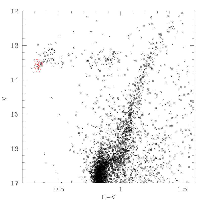
Figure 1: The CMD of M4 with the observed BHB stars indicated as open circles.

On the other hand almost all GCs observed to date (Carretta et al., 2009) show some kind of spread in their element content at the level of the RGB, the most evident being the spread in Na and O, elements that are anticorrelated (Carretta et al., 2010). Na and O abundances are also (anti)correlated with other light elements, such as C,N,Mg, and Al (Gratton et al., 2004).

The most natural explanation for this phenomenon is that clusters experienced an extended period of star formation, where the younger populations were born from an interstellar medium polluted by products of the CNO (and possibly NeNa, MgAl) cycle coming from massive stars of the former generation (Caloi & D’Antona, 2011, and reference therein). In this picture the interstellar medium is affected by an enhancement of its He content, together with N, Na, and Al, while C and O turn out to be depleted. This hypothesis can also explain correlations or anticorrelations of light elements present at the level of unevolved stars (Gratton et al., 2001). This phenomenon cannot be due to evolutionary effects like deep mixing processes that happen on the red giant branch (RGB) only after the first dredge-up (i.e. in stars brighter than the RGB-bump), since it is also present in MS stars.

Evidence for a direct correlation between the He and Na abundances is now accumulating. Bragaglia et al. (2010a) found differences in the abundances of Na as well as of other elements along the different main sequences of NGC 2808. In another paper Gratton et al. (2010), the same group found correlations between several expected features likely related to altered He abundances and the Na abundances for stars along the RGB for several clusters (the most clear evidence being again for NGC 2808). Very recently, Dupree et al. (2010) and Pasquini et al. (2011) observed that the chromospheric He I 10830 Å line is stronger in Na-rich RGB stars in $\omega$ Cen and NGC 2808, respectively, than in Na-poor stars.

Carretta et al. (2007) found that the extension of the Na-O anticorrelation is related to the extension of the horizontal branch (HB), suggesting that the anticorrelation may be related also to HB morphology.

Long ago Norris (1981), measuring the strength of the CN band at 3839 Å in M4, was the first to speculate on the possible connection between light-element and HB morphology in M4. Catelan & Freitas Pacheco (1995) were the first to speculate on the connection between super-oxygen-poor stars and blue HB morphology in M3 and M13.

It has been clear since the 1960s that the HB morphology is related not only to the cluster iron content (as expected from the models), but also to other parameters (the so called second parameter problem) which must account for the fact that some clusters have an HB extended or extremely extended to the blue, while others of the same metallicity do not.

Gratton et al. (2010) showed that the main candidate to be the second parameter is age. However they indicate also that at least a third parameter is required, and that it is most likely He.

A spread in He abundance can reproduce the HB morphology in GCs (as first noticed by Rood 1973) (see also the extensive analysis by Gratton et al. 2010). According to this picture, both stars with normal and enhanced He content end up on the zero-age horizontal branch (ZAHB) after the onset of core He burning. However, if mass loss in the previous phase is similar, He-rich stars should be less massive (and thus warmer) than He-normal ones because they burn H faster when they are on the main sequence. So He enhancement could provide the mechanism required to spread stars from the redder and cooler HB (stars with normal composition) to the hotter and bluer part of the HB (He-rich stars) as discussed in D’Antona et al. (2002).

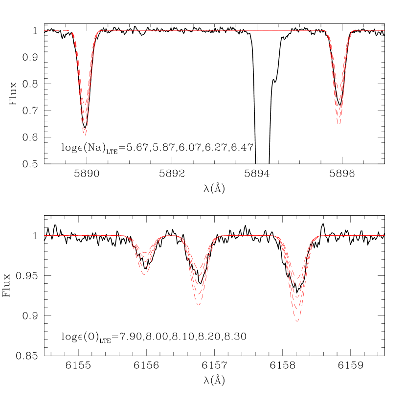
Figure 2: Example of Na (upper panel) and O (lower panel) spectral line fitting for the star #45025. Values for Na and O abundances of the synthetic spectra are indicated.

However, the most direct evidence, the spectroscopic determination of He abundances directly for the HB stars, is still scarce. Villanova et al. (2009, hereafter Vi09) analyzed a sample of stars in NGC 6752 belonging to the HB in the T_eff range between 8000 and 9000 K. As discussed in that paper only stars between 8500 and 11500 K are good targets for this purpose because they are sufficiently hot to show features of He in their spectra but cooler than the Grundahl-jump (Grundahl et al., 1999), the temperature limit above which stars show evidence of metal levitation and He sedimentation, which alters the original surface abundances (Pace at al., 2006). Vi09 found for all ZAHB stars of the redder part of the blue HB in NGC 6752 a Na-O content that, when compared with the Na-O anticorrelation found for the RGB (Carretta et al., 2009), demonstrates that they belong to the Na-poor and O-rich (primordial) population. The only evolved HB target, which likely comes from the bluer HB, belongs to the Na-rich, O-poor population. But, most important, they show that stars of the redder ZAHB are all Helium-normal (Y=0.25$\pm$0.01, where Y is the fractional mass of He), in agreement with the proposed scenario.

In addition, very recently (Marino et al., 2011) found a direct correlation between Na and O abundances and colours of the stars along the HB of M4. In fact, RHB stars are all Na-poor and O-rich, while BHB are all Na-rich and O-poor. According to this result we expect the BHB to be He-rich, and the RHB to be He-normal.

While all of this data point toward a connection between He spread and HB morphology, a key piece of information is still missing to finally confirm empirically this scenario. We need to verify whether ZAHB stars suitable for He measurement (8500$<$T${}_{\rm eff}<$11500 K) and belonging to the bluer HB indeed show a He-enhancement. The aim of this paper is to fill this gap by measuring the He content in blue HB (hereafter BHB) stars of M4 (NGC 6121). This cluster has been studied in detail (Marino et al., 2008). It has a bimodal HB with the hotter stars at T${}_{\rm eff}\sim$9500 K, and a bimodal Na-O anticorrelation, which is possibly related to a spread in He abundance. For this reason it is the ideal target for our purposes. We want to verify whether the hot HB stars of M4 are He-rich, as well as Na-rich/O-poor. In Section 2 we describe the observations. In Sec. 3 we discuss the determination of the atmospheric parameters of our stars and the line list we used. In Sec. 4, 5, 6, 7, 8, and 9 we present the spectroscopic and photometric analysis, compare our findings with the literature, and discuss and summarize our results.

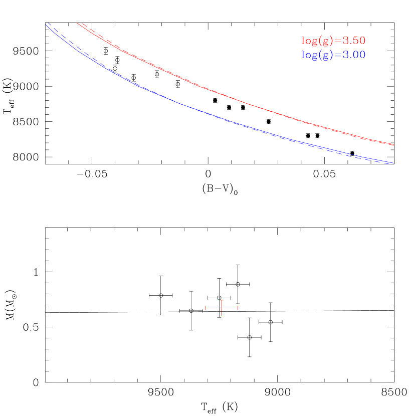
Figure 3: T_eff as a function of the B-V color (upper panel) and mass as a function of T_eff (lower panel) for our sample of stars (open circles). Filled circles are stars of NGC 6752 from Vi09 for comparison. In the upper panel our data are compared with Kurucz’s synthetic colors for different gravities. Continuous lines are synthetic colors for M4 metallicity, while dashed lines are synthetic colors for NGC 6752 metallicity. In the lower panel our data are compared with the theoretical mass (continuous line) for HB stars. The red cross is the mean value for our targets.

2 Observations, data reduction and membership

Observations of stars in the field of view of M4 were carried out in June-October 2009 in the context of the ESO Program ID 083.B-0083. In this program we observed a sample of 6 BHB stars (see Fig.1) for a total of 10$\times$45 min. exposures, selected from B,V photometry obtained by the WFI imager at the ESO2.2m telescope.
The selected targets have spectral type A0 ( ${\rm(B-V)_{0}\sim 0.0}$, T${\rm{}_{eff}\sim 9000}$ K ). This choice allows us to have targets showing He features in their spectrum, but not affected by levitation or sedimentation. Observations were performed with the FLAMES-UVES spectrograph at the VLT@UT2(Kueyen) telescope. Spectra of the candidate BHB stars were obtained using the 580nm setting with 1.0” fibers, and cover the wavelength range 4800-6800 Å with a mean resolution of R=47000.
Data were reduced using the UVES pipeline (Ballester et al., 2000), where raw data were bias-subtracted, flat-field corrected, extracted and wavelength calibrated. Echelle orders were flux calibrated using the master response curve of the instrument. Finally orders were merged to obtain a 1D spectrum and the spectra of each star sky-subtracted and averaged. Each spectrum has a mean S/N$\sim$150 per resolution element at 5875 Å.
The membership was established by radial velocity measurement. We used the fxcor IRAF utility to measure radial velocities. This routine cross-correlates the observed spectrum with a template having known radial velocity. As a template we used a synthetic spectrum calculated for a typical A0III star (T_eff=9000, log(g)=3.00, v_t=1.00 km/s, [Fe/H]=-1.5, roughly the same parameters as our stars). Spectra were calculated using the 2.76 version of SPECTRUM, the local thermodynamical equilibrium spectral synthesis program freely distributed by Richard O. Gray.
The error in radial velocity - derived from fxcor routine - is less than 1 km/s. Finally, for the abundance analysis, each spectrum was shifted to rest-frame velocity and continuum-normalized.
Table 1 lists the basic parameters of the selected stars: the ID, the J2000.0 coordinates (RA & DEC), V magnitude, B-V and U-V colors (Momany et al., 2003), heliocentric radial velocity (RV_H), T_eff, log(g), microturbulence velocity (v_t, for determination of atmospheric parameters see Sections 3 and 4). From the measured radial velocities we obtained a mean heliocentric radial velocity and a dispersion of:

${\rm<RV_{H}>=70.2\pm 2.6\ km/s},\ {\rm\sigma_{RV}=6.8\pm 1.8\ km/s}$

The mean velocity agrees well with literature values ( see e.g. Sommariva et al. (2009): ${\rm<RV_{H}>=70.3\ km/s}$ ). The dispersion we found is quite high, but also its error is large. It agrees within 2$\sigma$ with the more recent value derived in the literature (Peterson et al., 1995, 3.5$\pm$0.3 km/s). Considering the fact that at the position on the CMD of the target stars there is no significant background contamination, and that their [Fe/H] content agrees very well with the mean value for the cluster (see Section 4), we conclude that all the observed stars are cluster members.

Table 1: Basic parameters of the observed stars.

ID	RA(${\rm hh:mm:ss}$)	DEC(${\rm{}^{o}:\arcmin:\arcsec}$)	V(mag)	B-V(mag)	U-V(mag)	RVH(km/s)	Teff(K)	log(g)(dex)	vt(km/s)	vsini (km/s)
45025	16:23:34.380	-26:32:36.60	13.54	0.35	0.85	80.864	9030	3.30	1.57	9
46061	16:23:47.820	-26:32:06.00	13.47	0.32	0.77	75.784	9250	3.45	1.42	3
47570	16:23:34.760	-26:31:24.70	13.61	0.32	0.77	66.577	9370	3.45	1.02	7
49034	16:23:37.080	-26:30:44.60	13.61	0.31	0.73	62.305	9500	3.55	0.90	7
49412	16:23:36.300	-26:30:34.00	13.51	0.34	0.84	74.495	9170	3.52	1.50	5
50996	16:23:27.760	-26:29:49.00	13.70	0.33	0.78	66.677	9120	3.25	0.95	10

3 Atmospheric parameters, rotation and chemical abundances

We used the abundances from FeI/II features to obtain atmospheric parameters using the equivalent width (EQW) method.
None of our stars show evidence for strong rotation (see Table 1). For this reason EQWs are obtained from a Gaussian fit to the spectral features.
We could measure only a small number of Fe lines for each spectrum (5 FeI lines and 9 FeII lines) due to the limited spectral coverage. However the high quality of our spectra (allowing an accurate measurement of the EQWs) and the simultaneous use of both FeI/II sets of lines allowed us to obtain reliable atmospheric parameters, as confirmed by the comparison of theoretical and observational results (see below). The analysis was performed using the 2009 version of MOOG (Sneden, 1973) under a LTE approximation coupled with ATLAS9 atmosphere models (Kurucz, 1992).

T_eff was obtained by eliminating any trend in the relation of the abundances obtained from Fe I and Fe II lines with respect to the excitation potential (E.P.), while microturbulence velocity was obtained by eliminating any slope of the abundances obtained from FeI and FeII lines vs. reduced EQWs. log(g) values were estimated from the ionization equilibrium of FeI and FeII lines in order to have:

${\rm log\epsilon(FeI)=log\epsilon(FeII)}$

where $log\epsilon(El.)$=$log(N_{El.}/N_{H})+12$. N_El. and N_H are the density of the element and of hydrogen in number of particles per cm³. Adopted values for the atmospheric parameters are reported in Table 1.
All the targets, according to their position on the CMD, are consistent with being ZAHB objects (see Fig. 1).
The typical random error in T_eff and v_t can be obtained by the following procedure. First we calculated, for each star, the errors associated with the slopes of the best least squares fit in the relations between abundance vs. E.P. and reduced EQW. The average of the errors corresponds to the typical error on the slopes. Then, we selected one star representative of the entire sample (#46061). We fixed the other parameters and varied first temperature and then microturbulence until the slope of the line that best fits the relation between abundances and E.P. or reduced EQW becomes equal to the respective mean error. The amount of temperature and microturbulence variation represent an estimate of the random errors, that turned out to be 50 K and 0.04 km/s respectively. The error in gravity was estimated by satisfying the following equation:

${\rm{\tiny log\epsilon(FeI)-\Delta log\epsilon(FeI)=log\epsilon(FeII)+\Delta log\epsilon(FeII)}}$

where ${\rm\Delta log\epsilon(FeI)}$ and ${\rm\Delta log\epsilon(FeII)}$ are the errors on FeI/II abundance as given by MOOG. In other words we took the values ${\rm log\epsilon(FeI)}$ and ${\rm log\epsilon(FeII)}$ that satisfied the ionization equilibrium, decreased ${\rm log\epsilon(FeI)}$ and increased ${\rm log\epsilon(FeII)}$ by the errors given by MOOG, and estimated a new gravity using these new FeI/II abundances. The difference with the previous value was assumed to be our error on gravity, that turned out the be 0.06 dex on average. These errors are to be considered as random and internal. Systematic ones were checked as described in the next Section.

For a detailed description of the linelist we used for He, O, Na, and Fe and the solar value we adopted see Vi09. Suffice to say here that O and Na abundances were obtained by comparison with synthetic spectra from the O triplet at 6156-6158 Å and the Na doublet at 5889-5895 Å (see Fig. 2 for an example). Na and O are known to be affected by NLTE. For this reason, we applied the corrections by Takeda (1997) and Mashonkina et al. (2000), interpolated to the atmospheric parameters of our stars. On the other hand, as shown by Vi09, He abundances are not affected by NLTE, probably because the He line at 5875 Å, due to the very high E.P., is formed in very deep layers of the atmosphere, where departure from the LTE condition is negligible due to the high density of the gas. A further discussion is required about NLTE correction for Fe. Some authors (i.e. Qiu et al. 2001) claim that for A type stars like Vega or our targets a NLTE correction of +0.3 dex must be applied to FeI LTE abundances, while FeII are formed in LTE approximation. Slightly smaller non-LTE corrections have been recently estimated for such stars by Mashonkina (2011). All our tests show instead that no NLTE correction is required for FeI, at least down to log(g)=3.0. First of all, the analysis for Vega done in Vi09 assuming LTE gave us the same abundance for FeI and FeII within 0.02 dex, comparable with the r.m.s scatter. This result was confirmed by the analysis of the other targets of Vi09 and by Villanova et al. (2009b). In particular gravities of Vi09 were obtained from the wings of H Balmer lines, which are formed in LTE approximation. In spite of that no appreciable difference was found in the mean FeI and FeII abundances of the stars ($\Delta$[Fe/H]=0.04$\pm$0.05 dex).

There is a further effect to take into account. Our results indicate that all the stars are He-rich (Y$\sim$0.29, see next section). In spite of that for our analysis we used atmosphere models with normal He-content (Y$\sim$0.25). The question is whether this difference has some impact on the final abundances. We answered this by calculating with ATLAS9 a new He-enhanced atmosphere model for the star #46061, considered as representative of our sample. Then we recalculated the abundances. We found that O, Na, and Fe do not change in a significant way (0.01 dex or less). On the other hand, the He content changes by $\Delta$log$\epsilon$(He)=+0.03 dex. The reason could be that He lines form deep in the atmosphere where temperature is higher and the UV flux, strongly dominated by H and He opacity, is greater. This changes the structure of the atmosphere in the deepest layers and the strength of the spectral lines that are formed there. We took into account this effect by applying a correction $\Delta$log$\epsilon$(He)=+0.03 dex ($\Delta$Y=0.015) to the values for He obtained assuming He-normal atmosphere models.

Using spectral synthesis we could also measure projected rotational velocities for each star. For this purpose we assumed a combined instrumental+rotational profile for spectral features. The instrumental profile was assumed to be Gaussian with FWHM=R/$\lambda$ (where R is the resolution of the instrument). Then vsini was varied in order to match the observed profile of Na-double lines. Results are reported in Table 1. The typical error on vsini is 1-2 km/s (Villanova et al., 2009). The results confirm all these stars are relatively slow rotators

Table 2: Abundances obtained for the target stars.

El.	45025	46061	47570	49034	49412	50996
${\rm log\epsilon(He)}$	11.00	10.95	11.02	11.07	10.94	11.08
${\rm Y}$	0.28	0.26	0.30	0.32	0.26	0.32
${\rm[O/Fe]}$	0.34	0.36	0.30	0.34	0.27	0.38
${\rm[O/Fe]_{NLTE}}$	0.23	0.25	0.18	0.21	0.16	0.26
${\rm[Na/Fe]}$	0.82	0.85	0.69	0.66	0.73	0.61
${\rm[Na/Fe]_{NLTE}}$	0.47	0.55	0.39	0.37	0.40	0.28
${\rm[Fe/H]}$	-1.07	-1.06	-1.04	-1.04	-0.99	-1.13

Figure 4: Na-O abundances found for our HB targets (open circles). Filled circles are data for RGB stars from Marino et al. (2008). See Sec. 4 for more details.

4 Systematic errors

An estimation of the systematic errors (or at least upper limits) is very important for our purpose to compare our He abundance with the primordial value of the Universe.

First of all we checked our T_eff scale comparing the observed colors with synthetic B,V photometry, both from Kurucz. For this purpose we assumed an E(B-V)=0.36 value from Harris (1996). For Vi09 this test was not satisfying because temperatures from colors were very different from the spectroscopic ones. Meanwhile, we have further investigated this problem. By comparing our photometry, based on observations taken with the wide-field imager at the ESO2.2m telescope both for NGC 6752 and M4, with Stetson’s database (Stetson, 2000), we found that the blue and red parts of our CMDs are affected by photometric calibration problems, that can reach several hundredths of a magnitude. As a consequence we corrected our photometry and the result is plotted in Fig. 3 (upper panel). Empty circles are M4 stars, while filled ones are the old NGC 6752 data corrected for the reddening of the cluster. T_eff and dereddened B-V colors were compared with Kurucz synthetic photometry for log(g)=3.00 (blue) and 3.50 (red), which is roughly the gravity interval our stars cover. Continuous lines have [Fe/H]=-1.00, while dashed lines have [Fe/H]=-1.50 in order to cover the metal content of the two clusters. We note that colors in this temperature regime are very dependent on gravity but are almost unaffected by metallicity. The scatter for M4 stars is a bit higher than that for NGC 6752, due to the differential reddening affecting the former cluster.

If we compare T_eff from B-V colors with those obtained from spectroscopy for the two clusters, we find that for M4 the latter are underestimated by about 100 K, while for NGC 6752 they are overestimated by about 200 K. We are left with a net difference of 100 K. Part or all of this discrepancy is related to uncertainties in the value we adopted for the interstellar reddening, because even a small error of 0.01 mag would lead to an error of $\sim 150$ K in the effective temperatures. On average, the good agreement between temperatures from colours and from spectra is then comforting, and we can assume 150 K as un upper limit for the systematic error in temperature.

A better indication concerning the T_eff systematic errors comes from the comparison between our [Fe/H] (-1.06, see next section) with Marino et al. (2008, -1.07) and Marino et al. (2011, -1.12). First of all we note that both datasets were taken with the same instrument, so systematic effects on abundances due to the spectrograph (as happens for example comparing abundances measured with UVES and GIRAFFE, Carretta et al. 2009) can be ruled out. The difference is only 0.01 dex with respect to Marino et al. (2008) and 0.06 dex with respect to Marino et al. (2011). On the other hand, an error as large as 100 K on our spectroscopic T_eff would imply an offset of 0.10 dex. We can see that in the worst case comparison with Marino et al. (2011) gives 50 K as an estimate for our systematic error in temperature.

Finally Marino et al. (2011) checked the reliability of their atmospheric parameters comparing their T_eff with those derived from models by D’Antona et al. (2002). Their sample of stars distributes with a dispersion of $\sim$50 K and has a null offset with respect to the line of perfect agreement (see their Fig. 2). This implies a negligible systematic error on temparature, valid also for our data because in the two papers targets are similar and the methodology is the same.

After these tests we assume $\Delta$T_eff=50 K as the systematic error on our T_eff scale but we will consider also the upper limit $\Delta$T_eff$<$150 K in the discussion.

Systematic errors on our gravity scale can arise from the fact that we use FeI/II balance to obtain log(g). As said in the previous section this can introduce a systematic shift if FeI lines are formed in NLTE (while FeII lines form in LTE), as suggested by some authors. Thanks to our results on Vega and on other A stars presented in Vi09, we think we have shown that FeI lines can be safely treated with LTE approximation, and as a consequence systematic errors on the log(g) scale should be negligible.

This statement is further supported by Yuce et al. (2011). Here the authors analize a T_eff=12045 K, log(g)=3.9 dex star using Kurucz’s models, as in our case. They obtain atmospheric parameters from Strömgren photometry. As they say, ATLAS9 model with the parameters T_eff=12045 K, log(g)=3.9 derived from the Strömgren photometry meets the requirement of same iron abundance from all the different kinds of iron lines. In fact, they obtain the same abundance for FeI and FeII lines. If this is true for a 12000 K star, where NLTE effect (if present) should be larger than in our colder stars due to the stronger iron overionization, we can safely assume that LTE works well as an approximation for the atmosphere models of our targets, and it can be used to obtain unbiased gravities.

However we decided to perform further tests. For this purpose we calculated the mass ($\frac{M_{\star}}{M_{\odot}}$) of our stars by inverting the canonical equation:

${\rm log(\frac{g_{\star}}{g_{\odot}})=4\cdot log(\frac{T_{\star}}{T_{\odot}})-log(\frac{L_{\star}}{L_{\odot}})+log(\frac{M_{\star}}{M_{\odot}})}$

where

${\rm log(\frac{L_{\star}}{L_{\odot}})=-\frac{M_{bol}-4.74}{2.5}}$

and

${\rm M_{bol}=M_{V}+BC=V-(m-M)_{V}+BC}$

Bolometric correction (BC) was taken from Flower (1996), and distance modulus $(m-M)_{V}$ from Harris (1996). Results and relative errors are reported in Fig. 3 (lower panel) and compared with the theoretical model from Moni Bidin et al. (2007). The red cross is the mean value for our stars. It agrees very well with the theoretical value, well within 1$\sigma$. To match exactly the theoretical value we should change our log(g) scale by 0.03 dex.

After these tests we conclude that $\Delta$log(g)=0.05 dex is a reasonable value as the systematic error for our gravity scale.

We finally can estimate an upper limit for the systematic error on the He abundance. $\Delta$T_eff=50 K gives $\Delta$log$\epsilon$(He)=0.02 dex, and $\Delta$log(g)=0.05 dex again gives $\Delta$log$\epsilon$(He)=0.02. Those two values each translate into $\Delta$Y=0.01 and 0.01 respectively. The squared sum gives:

${\rm\Delta_{sys}(Y)=0.01\ (the\ exact\ value\ is\ 0.014)}$

which is our systematic error on the He abundance. If we consider the upper limit $\Delta$T_eff=150 K instead, we end up with:

${\rm\Delta_{sys}(Y)<0.03}$

Both values will be used in the discussion.

5 Results of the spectroscopic analysis

The chemical abundances we obtained are summarized in Table 2. From our sample the cluster turns out to have a Fe content of:

${\rm[Fe/H]=-1.06\pm 0.02}$

(internal error only) which agrees very well with the results from Marino et al. (2008) ([Fe/H]=-1.07$\pm$0.01). The agreement is slightly worse but within 0.06 dex with respect to Marino et al. (2011)([Fe/H]=-1.12).

In Fig. 4 we compare Na and O abundances for our target stars with the Na-O anticorrelation found by Marino et al. (2008) for a sample of M4 RGB stars. Marino et al. (2008) identified two separated populations in the Na-O plane, one O-rich and Na-poor, the other O-poor and Na-rich. We find that all our blue HB stars have a Na/O content which is fully compatible with the O-poor/Na-rich population. None of our targets belongs to the O-rich/Na-poor group. This is an indication that the light-element spread (Na and O in this case) is a vital clue to the morphology of the HB, and suggests that all O-rich/Na-poor objects end-up on the redder part of the ZAHB, while O-poor/Na-rich stars end-up on the bluer part of the ZAHB. We show this statistically by calculating the probability to find by chance six stars all belonging to the O-poor/Na-rich population, under the hypothesis that the HB morphology does not depend on the O/Na chemical content. Marino et al. (2008) show that the two populations in M4 contain about 50% of the total stars each. Under the previous hypothesis, we expect to find the blue HB to have an equal mixture of the two populations. The probability of finding 6 stars, all O-poor/Na-rich, as we found for the blue HB stars, is less than 2%. Therefore, we can conclude, at 98% confidence level, that the HB position does depend on the O/Na chemical content, or on a related factor, such as the He abundance.

A further confirmation of this assessment comes from Marino et al. (2011). In that paper we analyzed a large sample of stars of the two HBs in M4. For a subsample, observed with UVES, we could measure both O and Na, while for the remaining stars, observed with GIRAFFE and belonging to the red HB, only Na. We found that all the blue HB objects are O-poor/Na-rich, as in the present paper. On the other hand the two red HB stars with measured O are O-rich/Na-poor. All the remaining red HB stars for which we collected GIRAFFE spectra have Na that is compatible with the O-rich/Na-poor population. Again, the probability to find this result by chance is extremely low, in this case well below 1%.

The clear conclusion is that, at least for M4, the HB morphology is related to the light element content, specifically Na and O.

But a more important result regards the He content. In Fig. 5 we compare the observed spectra around the He line with 5 synthetic spectra with different He content. The stars turn out to have a mean He content of ${\rm log\epsilon(He)}$=11.01$\pm$0.02. This translates into:

${\rm Y=0.29\pm 0.01}$

In Tab. 2 logaritmic He abundances ${\rm log\epsilon(He)}$ for single stars were trasformed in mass fraction Y value as well. As noted before, our best estimation of the systematic error on the He measurement is:

${\rm\Delta_{sys}(Y)=0.01\ (or\ 0.014)}$

while the upper limit is:

${\rm\Delta_{sys}(Y)<0.03}$

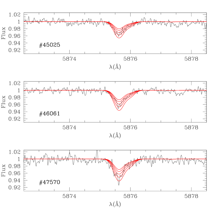
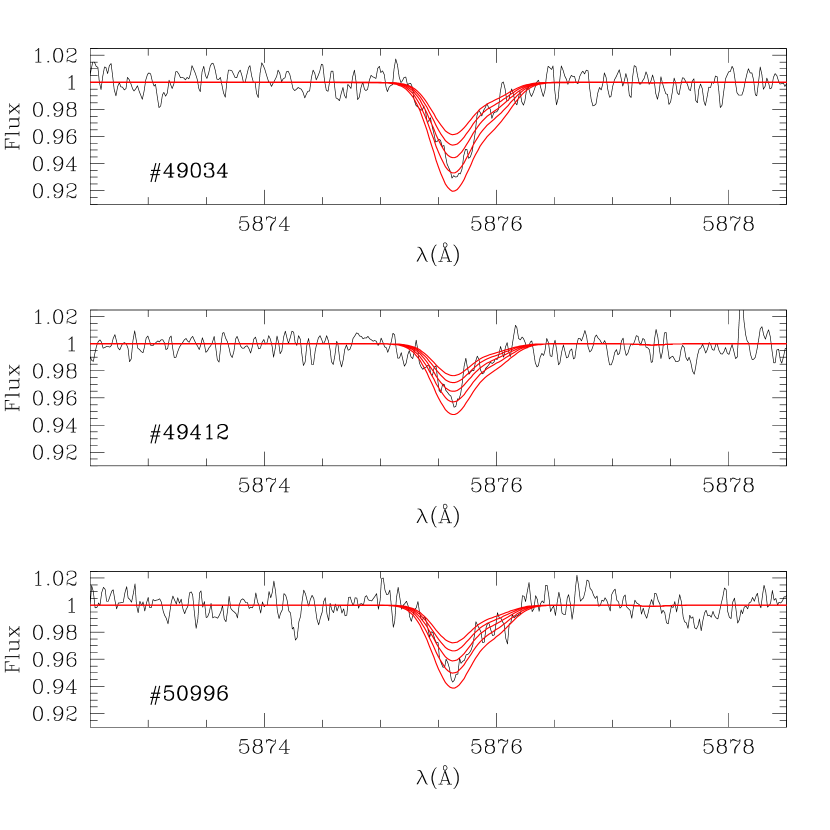
Figure 5: He lines of our stars. We superimposed on each observed spectrum 5 synthetic ones with log$\epsilon$(He)=10.70,10.80,10.90,11.00,11.10 respectively.

We conclude that the He content of our stars is larger than that of the primordial Universe (Y$\sim$0.24$\div$0.25) with a level of confidence of about 4$\sigma$ if we only consider the internal error. If we combine internal and systematic errors using the squared sum, the level of confidence is lower but still more than 2$\sigma$. It is less than 2$\sigma$ (between 1.3 and 1.6$\sigma$, depending on if we assume Y=0.24 or Y=0.25 for the primordial content) only if we use the upper limit for the systematic error. A possible point against the significance of our result comes from Sweigart (1987). This paper suggests that after the first dredge-up, the Y content of a star increases by $\sim$0.015 for Z=0.001 (roughly the metallicity of M4). So we should compare our absolute abundance with Y$\sim$0.24$\div$0.25+0.015$\sim$0.26. This would lower our significance to 1.7$\sigma$ (1.0$\sigma$ if we use the upper limit for the systematic error). However this He enhancement due to the first dredge-up is controversial, because other mechanisms (e.g. atomic diffusion, radiative acceleration, and turbulence) could be at work and playing a role in defining the precise He difference between MS and HB.

While not definitively proven, we believe our data strongly hints at a He abundance larger than the primordial value or than the value expected for a He-normal star after the first dredge-up. In the following, we will give various arguments that definitely support a similar conclusion.

First, we can compare the present results with the He content of HB stars of NGC 6752 found by Vi09. In both studies, we used the same spectrograph and methodology to estimate He abundance. Therefore, in such a comparison any systematic error is cancelled out. Vi09 found Y=0.25$\pm$0.01 for their sample of stars all belonging to the redder part of the blue HB of that cluster. Such a value is compatible with the primordial He abundance of the Universe. The stars of the present study are instead located on the bluer part of the HB of M4, and are then expected to be He-enhanced. The Y values of the two samples differ at the level of 2.8$\sigma$. We also applied a Kolmogorov-Smirnov test to the two datasets. This test concludes that the two distributions are not compatible, with a confidence level of more than 90%. We note that in this case the Sweigart (1987) result does not affect the comparison because BHB targets in both clusters should have experienced the same surface He-enhancement after the first dredge-up. Therefore we conclude that M4 BHB stars are He-enhanced.

We next compare M4 and NGC 6752 in more detail including O and Na. For this purpose we plot in Fig. 6 (upper panel) O and Na abundances from the following sources: M4 RGB stars (filled circles) from Marino et al. (2008), NGC 6752 RGB stars (stars) from Carretta et al . (2007b), M4 HB stars (open circles, this work), and NGC 6752 HB stars (open squares) from Villanova et al. (2009). We see that RGB stars of the two clusters define a common Na-O anticorrelation fitted by the curve. NGC 6752 stars cover a larger range both in O and Na. HB stars follow the same curve, as expected, but they map only a limited part of the anticorrelation, due to the fact that they are located in a restricted part of the HB. According to the results of this paper, the Na-O anticorrelation is accompanied by a He-O anticorrelation. This is shown in Fig. 6 (lower left panel). Red crosses are the mean values and errorbars for the two groups of stars, while the curve is the fit to the Na-O trend shifted and compressed in the y direction in order to match the observed points. This curve represents the He content that a stars has according to its Na abundance. In Fig. 6 (lower right panel) we report also the He-Na correlation. Again red crosses are the mean values and errorbars for the two groups, while the straight line is the fit to the data. This fit has the following form:

${\rm log\epsilon(He)=+0.14\pm 0.06\cdot[Na/Fe]+10.95\pm 0.02}$

In order to verify if these stars have also a homogeneous He content, we performed a detailed analysis of internal errors for this element. Helium was measured by comparing the observed spectrum with 5 synthetic ones, adopting the value that minimizes the r.m.s. scatter of the differences. The S/N of the real spectrum and the strength of the He line introduce an error in the final He abundance which can be estimated calculating the error on the r.m.s. scatter. For our data this error corresponds to uncertainties in the abundance of 0.06 dex. This value must be added to the errors due to the uncertainties on atmospheric parameters. As discussed before $\Delta$T_eff=50 K gives $\Delta$log$\epsilon$(He)=0.02 dex, $\Delta$log(g)=0.06 gives $\Delta$log$\epsilon$(He)=0.02 dex, while the error on microturbulence has no appreciable influence. The final uncertainty on the He abundance is given by the squared sum of all the individual errors, and the final result is $\Delta$log$\epsilon$(He)_tot=0.07 dex. If we compare this value to the observed dispersion (0.06$\pm$0.02 dex), we can conclude that our HB stars are compatible with having a homogeneous He content.

As discussed in the introduction, levitation and sedimentation are present in HB stars with temperatures hotter than 11500 K. As our stars are cooler, we expect that they are not affected by these phenomena. With the purpose of verifying this hypothesis we plotted log$\epsilon$(He), [El/Fe] and [Fe/H] vs. T_eff in Fig. 7. For each element we plotted the best fitting (continuous) and the $\pm$1$\sigma$ lines (dashed). All the elements show a trend that is flat within the errors.
Considering also that our abundances agree well with the RGB values of Marino et al. (2008), we conclude that none of the elements measured in the present paper show evidence of levitation or He sedimentation.

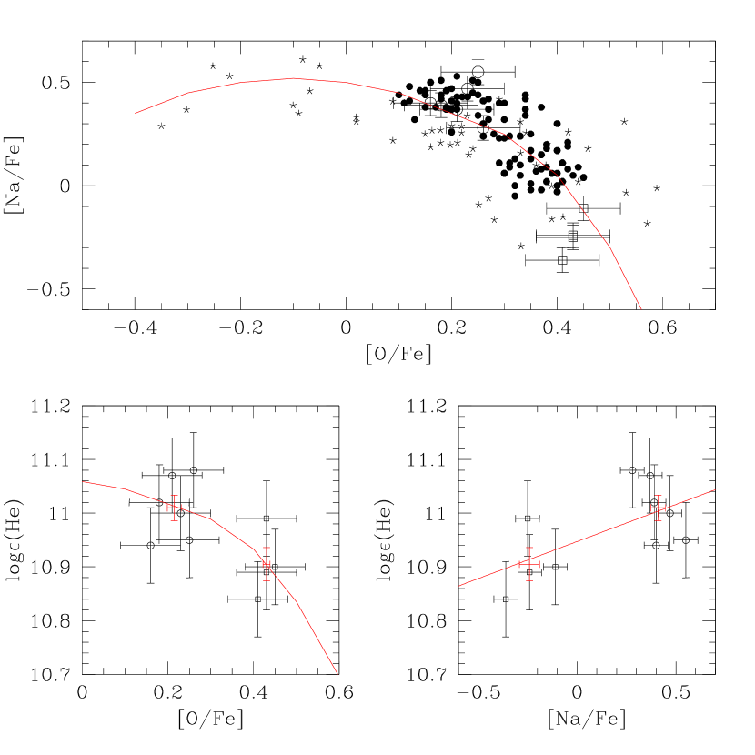
Figure 6: Upper panel: Na-O anticorrelation as defined by RGB and HB stars of M4 and NGC 6752. Lower left panel: He-O anticorrelation as defined by HB stars of M4 and NGC 6752. Lower right panel: He-Na correlation as defined by HB stars of M4 and NGC 6752. See text for more details

6 An independent photometric He estimation

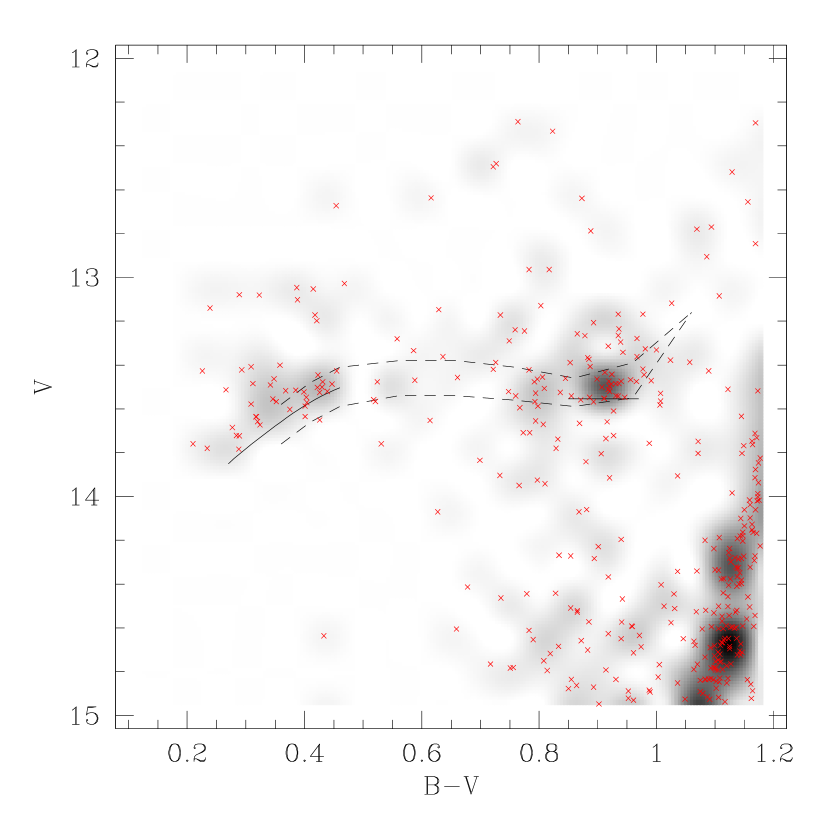
Figure 8: Hess diagram of the HB. Red and blue ZAHB (solid curves) were drawn by hand. Dashed are the ZAHB models by D’Antona et al. (2002) with Y=0.24 (the fainter) and Y=0.28 (the brighter). Single stars are shown as red crosses.

As noted by many authors (e.g. D’Antona et al. 2002), the brightness of the HB depends on the He content. The higher the He content, the brighter the HB. As our BHB stars are He enhanced, while the reddest HB stars in each cluster are expected to be He-normal (Y$\sim$0.25, as we found in NGC 6752), we also expect a difference in V magnitude between the two branches. The difference depends on the exact He difference, but for a value of the order of $\Delta$Y$\sim$0.04 suggested by our analysis, it should be of the order of $\sim$0.15 mag (Catelan et al., 2009). In order to verify this hypothesis we compared our photometry with zero age HB models by D’Antona et al. (2002). At this point the differential reddening affecting the cluster is a problem because it blurs out the exact HB location. To solve this issue we corrected the CMD for the differential reddening as explained in Sarajedini et al. (2007). Then, in order to locate exactly the HB, we built up the Hess diagram plotted in Fig. 8.

In this figure, the red HB is clearly visible as a bump at B-V=0.93, V=13.49, while the blue HB is the overdensity covering the range $0.25<$B-V$<0.45$ and $13.4<$V$<13.8$. We overplotted on both branches the HB lower envelope lines (the continuous lines) drawn to be 3$\times\Delta$V brighter than the faintest HB star, where $\Delta$V is the typical photometric error at the level of the HB. Dashed lines in the plot are the zero age HB models for the metallicity of the cluster by D’Antona et al. (2002) with Y=0.24 (fainter line) and Y=0.28 (brighter line). Models were shifted to the red by E(B-V)=0.36, and shifted in V in order to fit the lower envelope of the red HB with the model at Y=0.24. The model for Y=0.24 does not fit the lower envelope of the blue HB, which is brighter, as expected if it is He-enhanced. Then, we estimated the difference in V magnitude between the model at Y=0.24 and the blue HB ZAHB. It turned out to be $\sim$0.1 mag. This implies a difference in He of the two HBs of $\Delta$Y$\sim$0.02 according to the models of D’Antona et al. (2002), and of $\Delta$Y$\sim$0.03 according to (Catelan et al., 2009).

We conclude the photometric test further supports our contention that blue HB stars in M4 are He-enhanced (Y=0.29) with respect to the red HB by $\Delta$(Y)=0.02$\div$0.03.

Figure 7: log$\epsilon$(He), [O/Fe], [Na/Fe], and [Fe/H] vs. T_eff for our target stars in M4. For each element we plotted the best fitting (continuous) and the $\pm$1$\sigma$ lines (dashed)

7 Comparison with literature

Although we claim that M4 blue HB stars are He-enhanced, several previous papers found no evidence for this. The first is Behr (2003). Here the author obtained chemical abundances (including He) for a sample of blue HB stars around the Grundahl-jump for 6 clusters: M13, M15, M3, M68, M92, NGC288. In his Fig. 22 the author reports [He/H] value as a function of log(T_eff), and apparently this does not support our result about the He-enhancement because all stars cooler than the Grundahl-jump are compatible with a normal He content ([He/H]$\sim$0). However we wish to call attention to the following point. For three clusters (i.e. M13, M15, M92) the targets cooler than the Grundahl-jump belong to the reddest part of the HB so, as in the case of Villanova et al. (2009), they are indeed expected to be He-normal. Two of the remaining clusters (NGC288 and M68) do not have enough points below the Grundahl-jump to derive a firm conclusion. We are left with M3. The first impression from Fig. 22 of Behr (2003) is that these stars have a normal He content, but we immediately see that the errors are huge ($\sim$0.7 dex in the single measurement). Secondly, stars are located in the intermediate region of the HB (see Fig. 1 of Behr 2003), so their He-enhancement, if any, is expected to be close to the primordial value. Finally we point out that all Behr (2003) He measurements appear to be underestimated. For example M3 has a mean He content of [He/H]$\sim$-0.5, which translates into Y$\sim$0.10, clearly too low. The explication is that Behr (2003) was not interested in the absolute abundance of He as we are, but rather in the trend of He (among the other elements) with position along the HB. So he did not check possible systematic errors in his methods (e.g. the He linelist). For his purposes this was not necessary, but it makes a comparison with the present paper very problematic.

A second paper is Catelan et al. (2009). Here the authors compare the HB of M3 with theoretical models having different He content. They assert and show in their Fig. 2 and 3 that there is no evidence of He enhancement because the model with Y=0.25 fits well the HB. However, as Catelan et al. (2009) says, the fit is good, except perhaps for a small deviation of the lower envelope of the blue HB stars in the immediate vicinity of the ”knee” from the theoretical (single-Y) ZAHB.. The deviation is of $\sim$0.05 mag, with the stars brighter than the model. This value is small, but clearly visible and points toward a He-enhancement of blue HB stars in M3 with respect to red HB stars. We would have expected an even larger deviation for the bluest HB stars of the cluster which are expected to be even more He-rich, but in that region of the HB the models are degenerate. We can assert that Catelan et al. (2009), instead of contradicting our finding, actually supports it.

Finally Salaris et al. (2008) fit the HB of NGC 1851 with their theoretical models in order to obtain some hint about nature of the two populations of the clusters that were identified by Milone et al. (2008) as a bimodal SGB. They can fit the HB with two models. In the first the two populations are assumed to have an age difference of 1 Gyrs and the same (primordial) He, CNO, anf Fe content. In the second they are coeval and have different CNO (but the same primordial He and the same Fe). Apparently there is no room for an He-enhancement. First of all we notice that more recent papers (Villanova et al., 2010; Carretta et al., 2010b) found that stars in NGC 1851 have the same CNO content but different Fe ($\sim$0.06 dex). A difference in Fe have an impact on the age difference that is $\sim$0.5 Gyrs (assuming the same CNO). So none of the models by Salaris et al. (2008) is appropriate to fit the HB. On the other hand if we consider in their Fig. 2 (e.g. lower panel) the line that connect the red part with coolest part of the blue synthethic HB and project it on the observed HB (in order to fit the observed red HB), we can see that the observed blue HB is slightly brighter than this line. According to any HB model that assume the same CNO content (including Salaris et al. 2008, see their Fig. 1) this is an indication that the blue HB is He-enhancend with respect the red. This fact is confirmed by a recent paper (Gratton et al., 2012). Here the authors obtained a spectroscopic estimation of Y=+0.29$\pm$0.05 for the BHB. The error is quite large, but they show photometrically that the HB can be fitted only assuming Y=+0.248 and Y=+0.280 for the red and blue HBs respectivelly.

We conclude this section by noting that literature statements against the presence of He-rich stars in GCs are not conclusive, and that they are refuted by a new interpretation of the data or by new results.

8 Discussion

Correlations and anticorrelations of chemical elements observed in GCs (i.e. Na vs. O and Mg vs. Al) are attributed to contamination by products of the H-burning process at high temperature (Langer et al. 1993, Prantzos et al. 2007), when N is produced at the expense of O and C, and proton capture on Ne and Mg produces Na and Al (CNO, NeNa, and MgAl cycles). Gratton et al. (2001) demonstrated that this contamination is present also at the level of the MS. This means that it is not the result of a mixing mechanism present when a star leaves the MS, but it is rather due to primordial pollution of the interstellar material from which stars were formed. The mixing mechanism along the RGB can have an effect, but only as far as C and N are concerned (Gratton et al., 2000).

Pollution must come from more massive stars. GCs must have experienced some chemical evolution at the beginning of their life (see Gratton et al. 2004 for extensive references). The main product of H-burning is He and a He enhancement is then expected to be present in stars with an enhancement of N, Na, and Al. The main classes of candidate polluters are: fast-rotating massive main-sequence stars (Decressin et al., 2007), intermediate-mass AGB stars (D’Antona et al., 2002), and also massive binary stars (de Mink et al., 2009). All these channels can potentially pollute the existing interstellar material with products of complete CNO burning, including He (see Renzini 2008 for an extensive review).

Recently Villanova & Geisler (2011) showed that for M4 the best candidates that can reproduce the abundance pattern observed for RGB stars are massive main-sequence stars.

In the pollution scenario, a first generation of O-rich and Na-poor stars (relative to a second stellar generation) is formed from primordial homogeneous material, which must have been polluted by previous SN explosions. This generation also has a primordial or close to primordial He content (Y=0.24$\div$0.25). Then the most massive stars of this pristine stellar generation pollute the interstellar material with products of the CNO cycle. This material is kept in the cluster due to the relatively strong gravitational field (D’Ercole et al., 2008) , and it gives rise to a new generation of O-poor and Na-rich stars. This population should also have been He-enhanced (Y=0.27-0.35, depending on the major polluter and on the amount of retained material, D’Antona et al. 2002; Busso et al. 2007). Also the abundance of other elements (including s-process elements) may differ in stars of the first or second generation.

In the MS phase, He-rich stars evolve more rapidly than He-poor ones, so He/Na-rich (and O-poor) stars presently at the turn-off or in later phases of evolution should be less massive than He/Na-poor (and O-rich) ones. In this framework, D’Antona et al. (2002) and Carretta et al. (2007) proposed that a spread in He, combined with mass loss along the RGB, may be the main ingredient to naturally reproduce the whole HB morphology in GCs, as discussed in the introduction. According to this scenario, primordial He-O rich and Na poor stars end up on the redder part of the HB, while stars with extreme abundance alterations (strong He enhancement, O-poor and Na-rich) may end up on the bluer part of the HB, if they have experienced enough mass loss during the RGB phase. The extensive comparison between the distribution of colours along the HB and the Na-O anti-correlation by Gratton et al. (2010) also supports this view. Also age must play a role, because it determines the mean mass of a star that reaches the HB (Gratton et al., 2010; Dotter et al., 2010).

We stress that the HB represents the ideal locus to investigate the effects of chemical anomalies in GC stars, as the HB is a sort of amplifier of the physical conditions that are the consequence of the star composition and previous evolution.

In this scenario, in M4, we expect that the progeny of RGB He-normal, O-rich and Na-poor stars should reside in the red part of the HB. Therefore, it is not surprising that the observed red HB stars of Marino et al. (2011) are all O-rich, Na-poor. But they are too cold to have their He content measured directly. Marino et al. (2011) show also that blue HB stars are all O-poor and Na-rich. Here we reinforce this result with higher S/N spectra and more precise measurements. But we go further, measuring the He content of the blue HB. All our stars turned out to be He-enhanced (Y=0.29). By comparing photometry with HB models, we showed that the blue HB is brighter than the red, as expected if they have a different He content.

If we consider both the He and Na/O content of our targets, our result strongly confirms the hypothesis suggested by D’Antona et al. (2002), Carretta et al. (2007), Gratton et al. (2010), and shows that He (coupled with light-element spread) is one of the best candidates (together with the metal content and age) to explain the HB morphology of GCs and thus is a strong candidate for the 2^nd parameter (or for the 3^rd according to Gratton et al. 2010).

9 Summary

We studied a sample of BHB stars in M4 with a temperature in the range 9000-9500 K, with the aim of measuring their He and Na/O content. Targets were selected in order to be hot enough to show the He feature at 5875 Å, but cold enough to avoid the problem of He sedimentation and metal levitation affecting HB stars hotter than 11500 K. Thanks to the high resolution and high S/N of our spectra, we were able to measure He abundances for all our stars. This is only the second, direct measurement of He content from high resolution spectra of GC stars in this T_eff regime with the aim to test the current models of GC formation and multiple-populations.

Our sample of stars turns out to have [Fe/H]=-1.06$\pm$0.02, value that agrees well with the literature, and belong to the O-poor/Na-rich population of M4 found in the RGB region by Marino et al. (2008).

Our targets have a mean He content of Y=0.29
$\pm$0.01 (internal error) which is significantly larger than the value found for redder BHB stars in NGC 6752 (Y=0.25$\pm$0.01), using the same observational set up and data reduction procedures. Our best estimation for the systematic error is $\Delta$Y=0.01 (or 0.014). However it does not affect the comparison with NGC 6752 or the photometric estimation of the red HB He content. We compared also the brightness of the red and the blue HB of the cluster, finding that the latter is $\sim$0.1 mag brighter then the former. This result is quite strong, and we can estimate an enhancement in the He content for the stars in the blue vs. red HB of $\Delta$Y=0.02$\div$0.03. This is what we expect if stellar position on the HB is driven by its He and metal content. Our combined evidence strongly suggests that stars within the same globular cluster and among different globular clusters have different He content, and that the O-poor/Na-rich population is also He-enhanced with respect the O-rich/Na-poor population, as suggested by many theoretical studies. He is thus a leading contender for the 2^nd parameter.

Our results are consistent with theoretical studies which predict that, for a given metallicity and age, the position of a star in the HB is driven by its He content, and that the spread of stars along the HB must be related to the Na/O spread visible at the level of the RGB.

References

- Ballester et al. (2000) Ballester, P., Modigliani, A., Boitquin, O., Cristiani, S., Hanuschik, R., Kaufer, A., & Wolf, S. 2000, Msngr, 101, 31
- Bedin et al. (2004) Bedin, L.R., Piotto, G., Anderson, J., Cassisi, S., King, I.R., Momany, Y., & Carraro, G. 2004, ApJ, 605, 125
- Behr (2003) Behr, B.B. 2003, ApJSS, 149, 67
- Bragaglia et al. (2010a) Bragaglia, A., Carretta, E., Gratton, R.G., et al. 2010a, ApJ, 720, L41
- Bragaglia et al. (2010b) Bragaglia, A., Carretta, E., Gratton, R.G., et al. 2010b, A&A, 519, 60
- Busso et al. (2007) Busso, G., Cassisi, S., Piotto, G., Castellani, M., Romaniello, M., Catelan, M., Djorgovski, S.G., Recio Blanco, A., Renzini, A., Rich, M.R. 2007, A&A, 474, 105
- Caloi & D’Antona (2011) Caloi, V., & D’Antona, F. 2011, MNRAS, 417, 228
- Carretta et al. (2007) Carretta, E., Recio-Blanco, A., Gratton, R.G., Piotto, G., & Bragaglia, A. 2007, ApJ, 671, 125
- Carretta et al . (2007b) Carretta, E., Bragaglia, A., Gratton, R.G., Lucatello, S., & Momany, Y. 2007, A&A, 464, 927
- Carretta et al. (2009) Carretta, E., Bragaglia, A., Gratton, R.G., Lucatello, S., Catanzaro, G., Leone, F., Bellazzini, M., Claudi, R., D’Orazi, V., & Momany, Y. 2009, A&A, 505, 117
- Carretta et al. (2010) Carretta, E., Bragaglia, A., Gratton, R., Lucatello, S., Bellazzini, M., &D’Orazi, V. 2010, ApJ, 712, 21
- Carretta et al. (2010b) Carretta, E., Gratton, R.G., Lucatello, S., Bragaglia, A., Catanzaro, G., Leone, F., Momany, Y., D’Orazi, V., Cassisi, S., D’Antona, F., & Ortolani, S. 2010, ApJ, 722, 1
- Catelan & Freitas Pacheco (1995) Catelan, M., & de Freitas Pacheco, J.A. 1995, A&A, 297, 345
- Catelan et al. (2009) Catelan, M., Grundahl, F., Sweigart, A.V., Valcarce, A.A.R., & Cortés, C. 2009, ApJ, 695, 97
- D’Antona et al. (2002) D’Antona, F., Caloi, V., Montalbán, J., Ventura, P., & Gratton, R. 2002, A&A, 395, 69
- D’Antona et al. (2005) D’Antona, F., Bellazzini, M., Caloi, V., Fusi Pecci, F. , Galleti, S., & Rood, R. T. 2005, ApJ, 631, 868
- D’Antona & Ventura (2007) D’Antona, F. & Ventura, P. 2007, MNRAS, 379, 1431
- D’Ercole et al. (2008) D’Ercole, A., Vesperini, E., D’Antona, F., McMillan, S.L.W., & Recchi, S. 2008, MNRAS, 391, 825
- Decressin et al. (2007) Decressin, T., Meynet, G., Charbonnel, C., Prantzos, N., & Ekstrom, S. 2007, A&A, 464, 1029
- de Mink et al. (2009) de Mink, S E., Pols, O.R., Langer, N. & Izzard, R.G. 2009, A&A, 507, 1
- Dotter et al. (2010) Dotter, A., Sarajedini, A., Anderson, J., Aparicio, A., Bedin, L.R., Chaboyer, B., Majewski, S., Marín-Franch, A., et al. 2010, ApJ, 708, 698
- Dupree et al. (2010) Dupree, A.K., Strader, J., Smith, G. 2010, ApJ, in press (arXiv:1012:4802)
- Flower (1996) Flower, P.J. 1996, ApJ, 469, 355
- Gratton et al. (2000) Gratton, R.G., Sneden, C., Carretta, E., & Bragaglia, A. 2000, A&A, 354, 169
- Gratton et al. (2001) Gratton, R.G., Bonifacio, P., Bragaglia, A., Carretta, E., Castellani, V., Centurion, M., Chieffi, A., Claudi, R., Clementini, G., & D’Antona, F. 2001, A&A, 369, 87
- Gratton et al. (2004) Gratton, R., Sneden, C., & Carretta, E. 2004, ARA&A, 42, 385
- Gratton et al. (2010) Gratton, R.G., Carretta, E., Bragaglia, A., Lucatello, S., D’Orazi, V. 2010, A&A, 517, 81
- Gratton et al. (2012) Gratton, R.G., Lucatello, S., Carretta, E., Bragaglia, A., D’Orazi, V., Momany, Y., Sollima, A., Salaris, M., & Cassisi, S. 2012, arXiv:1201.1772
- Grundahl et al. (1999) Grundahl, F., Catelan, M., Landsman, W.B., Stetson, P.,B., & Andersen, M.I. 1999, ApJ, 524, 242
- Harris (1996) Harris, W.E. 1996, AJ, 112, 1487
- Kurucz (1992) Kurucz, R.L. 1992, IAUS, 149, 225
- Langer et al. (1993) Langer, G.E., Hoffman, R., & Sneden, C. 1993, PASP, 105, 301
- Marino et al. (2008) Marino, A.F., Villanova, S., Piotto, G., Milone, A.P., Momany, Y., Bedin, L.R., & Medling, A.M. 2008, A&A, 490, 625
- Marino et al. (2011) Marino, A. F., Villanova, S., Milone, A. P., Piotto, G., Lind, K., Geisler, D. & Stetson, P. B. 2011, ApJ, 730, 16
- Mashonkina (2011) Mashonkina, L.I., 2011, arXiv:1104.4403
- Mashonkina et al. (2000) Mashonkina, L.I., Shimanskii, V. V., & Sakhibullin, N.A. 2000, ARep, 44, 790
- Milone et al. (2008) Milone, A.P., Bedin, L.R., Piotto, G., Anderson, J., King, I.R., Sarajedini, A., Dotter, A., Chaboyer, B., Marín-Franch, A., Majewski, S. 2008, ApJ, 673, 241
- Momany et al. (2003) Momany, Y., Cassisi, S., Piotto, G., Bedin, L.R., Ortolani, S., Castelli, F., & Recio-Blanco, A. 2003, A&A, 407, 303
- Moni Bidin et al. (2007) Moni Bidin, C., Moehler, S., Piotto, G., Momany, Y., & Recio-Blanco, A. 2007, A&A, 474, 505
- Norris (1981) 1981, ApJ, 248, 177
- Norris (2004) Norris, J.E. 2004, ApJ, 612, 25
- Pace at al. (2006) Pace, G., Recio-Blanco, A., Piotto, G. & Momany, Y. 2006, A&A, 452, 493
- Pasquini et al. (2011) Pasquini, L., Mauas, P., Kaufl, H.U., Cacciari, C. 2011, A&A, in press (arXiv:1105:0346)
- Peterson et al. (1995) Peterson, R.C., Rees, R.F., & Cudworth, K.M. 1995, ApJ, 443, 124.
- Piotto et al. (2005) Piotto, G., Villanova, S., Bedin, L.R., Gratton, R., Cassisi, S., Momany, Y., Recio-Blanco, A., Lucatello, S., Anderson, J., & King, I.R. 2005, ApJ, 621, 777
- Piotto et al. (2007) Piotto, G., Bedin, L.R., Anderson, J., King, I.R., Cassisi, S., Milone, A.P., Villanova, S., Pietrinferni, A., & Renzini, A. 2007, ApJ, 661, 53
- Prantzos et al. (2007) Prantzos, N., Charbonnel, C., & Iliadis, C. 2007, A&A, 470, 179
- Pryor & Meylan (1993) Pryor, C. & Meylan, G. 1993, ASPC, 50, 357
- Qiu et al. (2001) Qiu, H.M., Zhao, G., Chen, Y.Q., Li, Z.W. & 2001, ApJ, 548, 953
- Renzini (2008) Renzini, A. 2008, MNRAS, 391, 354
- Rood (1973) Rood, R.T. 1973, ApJ, 184, 815
- Salaris et al. (2008) Salaris, M., Cassisi, S., & Pietrinferni, A. 2008, ApJ, 678, 25
- Sarajedini et al. (2007) Sarajedini, A., Bedin, L.R., Chaboyer, B., Dotter, A., Siegel, M., Anderson, J., Aparicio, A., King, I., Majewski, S.,; Marín-Franch, A., Piotto, G., Reid, I.N., Rosenberg, A. 2007, AJ, 133, 1658
- Sneden (1973) Sneden, C. 1973, ApJ, 184, 839
- Sommariva et al. (2009) Sommariva, V., Piotto, G., Rejkuba, M., Bedin, L.R., Heggie, D.C., Mathieu, R.D., & Villanova, S. 2009, A&A, 493, 947
- Stetson (2000) Stetson, P.B. 2000, PASP, 112, 925
- Sweigart (1987) Sweigart, A.V. 1997, ApJS, 65, 95
- Takeda (1997) Takeda, Y. 1997, PASJ, 49, 471
- Yuce et al. (2011) Yuce, K., Castelli, F., & Hubrig, S. 2011, A&A, 528, 37,
- Villanova et al. (2007) Villanova, S., Piotto, G., King, I.R., Anderson, J., Bedin, L.R., Gratton, R.G., Cassisi, S., Momany, Y., Bellini, A., & Cool, A.M. 2007, ApJ, 663, 296
- Villanova et al. (2009) Villanova, S., Piotto, G., & Gratton, R.G. 2009, A&A, 499, 755
- Villanova et al. (2009b) Villanova, S., Carraro, G., & Saviane, I. 2009, A&A, 504, 845
- Villanova et al. (2010) Villanova, S., Geisler, D., & Piotto, G. 2010, ApJ, 722, 18
- Villanova & Geisler (2011) Villanova, S., & Geisler, D. 2011, arXiv1109.0973