Atom and photon measurement in cooperative scattering by cold atoms

Abstract

In this paper, we study cooperative scattering of low intensity light by a cloud of N two-level systems. We include the incident laser field driving these two-level systems and compute the radiation pressure force on the center of mass of the cloud. This signature is of particular interest for experiments with laser cooled atoms. Including the complex coupling between dipoles in a scalar model for dilute clouds of two-level systems, we obtain expression for cooperative scattering forces taking into account the collective Lamb shift. We also derive the expression of the radiation pressure force on a large cloud of two-level systems from an heuristic approach and show that at lowest driving intensities this force is identical for a product and an entangled state.

I Introduction

Cooperative scattering by an assembly of resonant systems has been studied in detail for many years and is based on the seminal work by R. Dicke in 1954 Dicke54 . Related superradiance effects and collective level shifts have been studied in the context of atomic physics in the 70s Lehmberg68 ; Friedberg ; Gross82 . In the last decade, this topic has seen renewed interest Eberly06 ; Scully06 ; Friedberg07 ; Svidzinsky08 ; Scully09 ; Scully09LS ; Svi10 ; Friedberg10 ; Friedberg10b ; Prasad10 with novel experiments in nuclear physics Rohlsberger10 and in laser cooled clouds of atoms Bienaime10 ; Bender10 ; Courteille10 ; Kaiser09 ; Bux10 , applications in quantum information Greentree06 and quantum phase transitions Osterloh02 ; Akkermanns08 . As we are mainly concerned with applications on laser cooled atomic samples, we focus in this paper on specific parameters and observables which are of interest in such experiments. We therefore derive expressions of the radiation pressure force acting on the center of mass of the atomic cloud, as well as the scattered electric field. We go beyond past approximations including the complex kernel for the coupling terms between N atoms Friedberg ; Svidzinsky08 , described by two-level systems in a scalar approach. Neglecting the complete vectorial nature of the dipole dipole coupling seems a priori more justified in a dilute sample of atoms, where near field corrections are small Kaiser09 . Furthermore, we obtain the force and the radiation field as quantum operators, which may be useful for studying fluctuations and diffusion effects in radiation forces and scattered emission. Also, the imaginary part of the complex kernel, describing the collective Lamb shift, is evaluated for a gaussian density profile.

This paper is organized as follows: in section II, we specify the Hamiltonian used and discuss our approximations. In section III, we introduce the observables relevant for experiments with cold atoms, namely the radiation pressure forces on the center of mass of the atomic cloud and the scattered light intensity. The evaluation of these observables is done for specific atomic states in section IV. We derive the result for this cooperative radiation pressure force from a more heuristic approach in section V. In section VI we discuss the relevance of the Timed Dicke State compared to a product state for this cooperative pressure force in the low intensity limit before concluding in section VII.

II Hamiltonian and operator equations

Our system consists of a gas of $N$ two-level atoms (with random positions $\mathbf{r}_{j}$, lower and upper states $|g_{j}\rangle$ and $|e_{j}\rangle$ with $j=1,\dots,N$, transition frequency $\omega_{a}$ with linewidth $\Gamma=d^{2}\omega_{a}^{3}/2\pi\hbar\epsilon_{0}c^{3}$, where $d$ is the electric dipole matrix element), driven by a uniform resonant radiation beam with wave vector $\mathbf{k}_{0}=k_{0}\mathbf{\hat{e}}_{z}$, frequency $\omega_{0}=\omega_{a}+\Delta_{0}$ and electric field $E_{0}$ (see fig. 1).

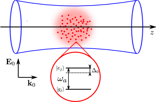
Figure 1: (color online) Experimental configuration considered : a cloud of two-level atoms is driven by an incident laser detuned by $\Delta_{0}$ from the atomic resonance $\omega_{a}$, with wavevector $\mathbf{k}_{0}$.

The atom-field interaction Hamiltonian in the rotating-wave approximation (RWA) is

$$\hat{H}=\hat{H}_{0}+\hat{H}_{1}$$ (1)

where

$$\hat{H}_{0} = \hbar\sum_{j=1}^{N}\left\{-\frac{\Delta_{0}}{2}\hat{\sigma}_{3j}+\frac{\Omega_{0}}{2}\left(\hat{\sigma}_{j}e^{-i\mathbf{k}_{0}\cdot\mathbf{r}_{j}}+{\hat{\sigma}_{j}}^{\dagger}e^{i\mathbf{k}_{0}\cdot\mathbf{r}_{j}}\right)\right\}$$

$$\hat{H}_{1} = \hbar\sum_{j=1}^{N}\sum_{\mathbf{k}}g_{k}\left[\hat{a}_{\mathbf{k}}^{\dagger}\hat{\sigma}_{j}e^{i(\omega_{k}-\omega_{0})t-i\mathbf{k}\cdot\mathbf{r}_{j}}+{\hat{\sigma}_{j}}^{\dagger}\hat{a}_{\mathbf{k}}e^{-i(\omega_{k}-\omega_{0})t+i\mathbf{k}\cdot\mathbf{r}_{j}}\right].$$ (2)

Here $\Omega_{0}=dE_{0}/\hbar$ is the pump Rabi frequency, $\hat{a}_{\mathbf{k}}$ is the photon annihilation operator with wavenumber $\mathbf{k}$ and frequency $\omega_{k}=ck$, $g_{k}=d\sqrt{\omega_{k}/(2\hbar\epsilon_{0}V_{ph})}$, $V_{ph}$ the photon volume, $\hat{\sigma}_{j}=\exp(i\Delta_{0}t)|g_{j}\rangle\langle e_{j}|$ and $\hat{\sigma}_{3j}=|e_{j}\rangle\langle e_{j}|-|g_{j}\rangle\langle g_{j}|$. Instead of solving the Schrödinger equation introducing some ansatz for the system state $|\Psi(t)\rangle$ Courteille10 , we write the motion equations of the atomic and field operators,

$$\frac{d\hat{\sigma}_{j}}{dt} = \frac{1}{i\hbar}[\hat{\sigma}_{j},\hat{H}]=i\Delta_{0}\hat{\sigma}_{j}+\frac{i\Omega_{0}}{2}\hat{\sigma}_{3j}e^{i\mathbf{k}_{0}\cdot\mathbf{r}_{j}}+i\sum_{\mathbf{k}}g_{k}\hat{\sigma}_{3j}\hat{a}_{\mathbf{k}}e^{-i(\omega_{k}-\omega_{0})t+i\mathbf{k}\cdot\mathbf{r}_{j}}$$ (3)

$$\frac{d\hat{\sigma}_{3j}}{dt} = \frac{1}{i\hbar}[\hat{\sigma}_{3j},\hat{H}]=i\Omega_{0}\hat{\sigma}_{j}e^{-i\mathbf{k}_{0}\cdot\mathbf{r}_{j}}+2i\sum_{\mathbf{k}}g_{k}\hat{a}_{\mathbf{k}}^{\dagger}\sigma_{j}e^{i(\omega_{k}-\omega_{0})t-i\mathbf{k}\cdot\mathbf{r}_{j}}+\textrm{h.c.}$$ (4)

$$\frac{d\hat{a}_{\mathbf{k}}}{dt} = \frac{1}{i\hbar}[\hat{a}_{\mathbf{k}},\hat{H}]=-ig_{k}e^{i(\omega_{k}-\omega_{0})t}\sum_{m=1}^{N}\hat{\sigma}_{m}e^{-i\mathbf{k}\cdot\mathbf{r}_{m}}.$$ (5)

We consider the atoms initially in their ground state and we assume weak excitation ($\Omega_{0}\ll\Gamma$), so that we approximate $\hat{\sigma}_{3j}(t)\approx-\hat{I}_{j}$, where $\hat{I}_{j}$ is the identity operator for the $j$th atom. This approximation amounts to neglect saturation and multi-excitation, i.e. all the processes generating more than one photon at the same time (linear regime). Integrating Eq.(5) and substituting it into Eq.(3), neglecting $a_{k}(0)$ (since the initial field state is vacuum) we obtain

$$\frac{d\hat{\sigma}_{j}}{dt} = i\Delta_{0}\hat{\sigma}_{j}-\frac{i\Omega_{0}}{2}\hat{I}_{j}e^{i\mathbf{k}_{0}\cdot\mathbf{r}_{j}}-\sum_{\mathbf{k}}g_{k}^{2}\sum_{m=1}^{N}e^{i\mathbf{k}\cdot(\mathbf{r}_{j}-\mathbf{r}_{m})}\int_{0}^{t}dt^{\prime}\hat{\sigma}_{m}(t-t^{\prime})\,e^{-i(\omega_{k}-\omega_{0})t^{\prime}}.$$ (6)

The last term in Eq.(6) describes the effect of the spontaneously emitted photons on the atoms, and it is well known in the quantum electrodynamic literature Scully:QO ; Agarwal . In the Markov approximation (i.e. when the photon transit time through the atomic sample is much shorter than the excitation decay time velocity ), we assume under the integral $\hat{\sigma}_{m}(t-t^{\prime})\approx\hat{\sigma}_{m}(t)$. The time integral then yields a real part (with a term $\delta(k-k_{0})$ ) and an imaginary part (corresponding to the principal part of the integral). Taking into account these two terms is at the origin of the exponential kernel whereas the real part alone would lead to a sin kernel in Eq.(9) below. We then transform the sum over the modes $\mathbf{k}$ into an integral, $\sum_{\mathbf{k}}\rightarrow(V_{ph}/8\pi^{3})\int d\mathbf{k}$. The real and imaginary parts of the double integral over $t$ and $\mathbf{k}$ yield the cooperative decay and frequency shift (collective Lamb shift), respectively. The proper expression of the cooperative frequency shift has been obtained adding to the Hamiltonian (2) the not-RWA contributions associated to virtual photons exchanged between different atoms. It results the following relation Svi10 :

$$\sum_{\mathbf{k}}g_{k}^{2}e^{i\mathbf{k}\cdot\mathbf{R}}\int_{0}^{\infty}dt^{\prime}e^{-ic(k-k_{0})t^{\prime}}\longrightarrow\frac{\Gamma}{2ik_{0}|\mathbf{R}|}e^{ik_{0}|\mathbf{R}|}$$ (7)

where $\Gamma=V_{ph}g_{k_{0}}^{2}k_{0}^{2}/(\pi c)$. Using Eq.(7) in Eq.(6) we obtain Svi10 ,

$$\frac{d\hat{\sigma}_{j}(t)}{dt} = i\Delta_{0}\hat{\sigma}_{j}(t)-\frac{i\Omega_{0}}{2}\hat{I}_{j}e^{i\mathbf{k}_{0}\cdot\mathbf{r}_{j}}-\frac{\Gamma}{2}\sum_{m=1}^{N}\gamma_{jm}\hat{\sigma}_{m}(t).$$ (8)

where

$$\gamma_{jm}=\frac{-i\cos(k_{0}r_{jm})+\sin(k_{0}r_{jm})}{k_{0}r_{jm}}=\frac{e^{ik_{0}r_{jm}}}{ik_{0}r_{jm}}.$$ (9)

and $r_{jm}=|\mathbf{r}_{j}-\mathbf{r}_{m}|$. Eqs.(8) describe the time evolution of the atomic operators for $N$ weakly excited atoms scattering radiation. The real part of $\gamma_{jm}$ describes the spontaneous emission decay and the imaginary part of $\gamma_{jm}$ describes the energy shift due to resonant dipole-dipole interactions. A slightly different approach can be used to derive this result as shown in appendix A. Note that even though this result will yield a density dependent collective shift of the resonance, we use a scalar model for the field, neglecting thus any polarization and near field dependence Scully09LS ; Friedberg10 . Detailed calculations for small and large samples of various geometries however show that near field and far field contributions as well as resonant and antiresonant terms need to be taken properly into account for quantitative predictions Friedberg ; Friedberg10 ; Friedberg10b , and the present model thus needs to be considered with care illustrating only a part of the dipole-dipole coupling for real systems.

Eq.(8) can also cast in the form

$$\frac{d\hat{\sigma}_{j}}{dt} = \frac{1}{i\hbar}[\hat{\sigma}_{j},\hat{H}_{0}^{\prime}+\hat{H}_{eff}],$$ (10)

where

$${\hat{H}_{0}}^{\prime} = \hbar\sum_{j=1}^{N}\left\{-\Delta_{0}\hat{\sigma}^{\dagger}_{j}\hat{\sigma}_{j}+\frac{\Omega_{0}}{2}\left(\hat{\sigma}_{j}e^{-i\mathbf{k}_{0}\cdot\mathbf{r}_{j}}+{\hat{\sigma}_{j}}^{\dagger}e^{i\mathbf{k}_{0}\cdot\mathbf{r}_{j}}\right)\right\}$$

$$\hat{H}_{eff} = \frac{\hbar\Gamma}{2}\sum_{j,m}\frac{e^{ik_{0}r_{jm}}}{ik_{0}r_{jm}}\hat{\sigma}_{j}^{\dagger}\hat{\sigma}_{m}.$$ (11)

and the commutation rules in the linear regime are $[\hat{\sigma}_{j},\hat{\sigma}_{m}^{\dagger}]=\delta_{jm}$.

III Observables

Among the different observables of the system, scattered light and radiation pressure force contain important signatures of cooperative scattering. Concerning scattered radiation, the positive-frequency part of the electric field is defined as

$$\hat{E}(\mathbf{r},t)=i\sum_{\mathbf{k}}{\cal E}_{k}\hat{a}_{\mathbf{k}}(t)e^{-i\omega_{k}t+i\mathbf{k}\cdot\mathbf{r}}$$ (12)

where ${\cal E}_{k}=\sqrt{\hbar\omega_{k}/2\epsilon_{0}V_{ph}}$ is the single-photon electric field. By integrating Eq.(5) and inserting it in Eq.(12) we obtain

$$\hat{E}(\mathbf{r},t)=\sum_{\mathbf{k}}{\cal E}_{k}g_{k}\sum_{m=1}^{N}e^{i\mathbf{k}\cdot(\mathbf{r}-\mathbf{r}_{m})-i\omega_{0}t}\int_{0}^{t}dt^{\prime}e^{-i(\omega_{k}-\omega_{0})t^{\prime}}\hat{\sigma}_{m}(t-t^{\prime})$$ (13)

Using Eq.(7), the Markov approximation leads to

$$\hat{E}(\mathbf{r},t)\approx-i\frac{dk_{0}^{2}}{4\pi\epsilon_{0}}\sum_{j=1}^{N}\frac{e^{-i\omega_{0}(t-|\mathbf{r}-\mathbf{r}_{j}|/c)}}{|\mathbf{r}-\mathbf{r}_{j}|}\hat{\sigma}_{j}(t)$$ (14)

which has a transparent interpretation as the sum of wavelets scattered by $N$ dipoles of position $\mathbf{r}_{j}$ and detected at distance $\mathbf{r}$ and time $t$. In the far field limit, $|\mathbf{r}-\mathbf{r}_{j}|\approx r-(\mathbf{r}\cdot\mathbf{r}_{j})/r$ and

$$\hat{E}(\mathbf{r},t)\approx-i\frac{dk_{0}^{2}}{4\pi\epsilon_{0}r}e^{-i\omega_{0}(t-r/c)}\sum_{j=1}^{N}e^{-i\mathbf{k_{s}}\cdot\mathbf{r}_{j}}\hat{\sigma}_{j}(t)$$ (15)

where $\mathbf{k}_{s}=k_{0}(\mathbf{r}/r)$.

The radiation pressure force acting on the $j$th-atom has been calculated from Eq.(1) as $\hat{\mathbf{F}}_{j}=-\nabla_{\mathbf{r}_{j}}\hat{H}=\hat{\mathbf{F}}_{aj}+\hat{\mathbf{F}}_{ej}$ where Courteille10

$$\hat{\mathbf{F}}_{aj} = i\hbar\mathbf{k}_{0}\frac{\Omega_{0}}{2}\left\{e^{-i\mathbf{k}_{0}\cdot\mathbf{}r_{j}}\hat{\sigma}_{j}-\textrm{h.c.}\right\}$$ (16)

$$\hat{\mathbf{F}}_{ej} = i\hbar\sum_{\mathbf{k}}\mathbf{k}g_{k}\left\{\hat{a}_{\mathbf{k}}^{\dagger}\hat{\sigma}_{j}e^{i(\omega_{k}-\omega_{0})t-i\mathbf{k}\cdot\mathbf{r}_{j}}-\hat{\sigma}_{j}^{\dagger}\hat{a}_{\mathbf{k}}e^{-i(\omega_{k}-\omega_{0})t+i\mathbf{k}\cdot\mathbf{r}_{j}}\right\}$$ (17)

where $\hat{\mathbf{F}}_{aj}$ and $\hat{\mathbf{F}}_{ej}$ result from the recoil received upon absorption of a photon from the pump and from the emission of a photon into any direction $\mathbf{k}$, respectively. Eliminating the field using Eq.(5), Eq.(17) becomes

$$\hat{\mathbf{F}}_{ej}(t)=-\hbar\sum_{\mathbf{k}}\mathbf{k}g_{k}^{2} \left\{\sum_{m=1}^{N}e^{-i\mathbf{k}\cdot(\mathbf{r}_{j}-\mathbf{r}_{m})}\int_{0}^{t}dt^{\prime}e^{i(\omega_{k}-\omega_{0})t^{\prime}}\hat{\sigma}_{m}^{\dagger}(t-t^{\prime})\,\hat{\sigma}_{j}(t)\right.$$ (18)

$$+\left.\hat{\sigma}_{j}^{\dagger}(t)\sum_{m=1}^{N}e^{i\mathbf{k}\cdot(\mathbf{r}_{j}-\mathbf{r}_{m})}\int_{0}^{t}dt^{\prime}e^{-i(\omega_{k}-\omega_{0})t^{\prime}}\hat{\sigma}_{m}(t-t^{\prime})\right\}.$$

Assuming the Markov approximation, $\hat{\sigma}_{m}(t-t^{\prime})\approx\hat{\sigma}_{m}(t)$, then Eq.(18) becomes

$$\hat{\mathbf{F}}_{ej}(t) = -\hbar\sum_{m=1}^{N}\sum_{\mathbf{k}}\mathbf{k}g_{k}^{2}\left\{\hat{\sigma}_{m}^{\dagger}(t)\hat{\sigma}_{j}(t)e^{-i\mathbf{k}\cdot\mathbf{r}_{jm}}\int_{0}^{t}dt^{\prime}e^{i(\omega_{k}-\omega_{0})t^{\prime}}+\hat{\sigma}_{j}^{\dagger}(t)\hat{\sigma}_{m}(t)e^{i\mathbf{k}\cdot\mathbf{r}_{jm}}\int_{0}^{t}dt^{\prime}e^{-i(\omega_{k}-\omega_{0})t^{\prime}}\right\}$$ (19)

where $\mathbf{r}_{jm}=\mathbf{r}_{j}-\mathbf{r}_{m}$. The force (19) acting on the $j$th atom has a single-atom contribution $\hat{\mathbf{F}}_{ej}^{(\textrm{self})}$ (term $m=j$ in the sum) accounting for its own photon emission recoil, and a contribution $\hat{\mathbf{F}}_{ej}^{(\textrm{int})}$ (terms $m\neq j$) accounting for coupling between the $j$th atom and all the other atoms. Note that this dipole-dipole interaction can occur via a coupling to common vacuum modes of radiation. The interference terms in the total scattered field can leave a fingerprint on the forces acting on the atoms inside the cloud. The first contribution yields

$$\hat{\mathbf{F}}_{ej}^{(\textrm{self})} \approx -\hbar\Gamma\sum_{|\mathbf{k}|=k_{0}}\mathbf{k}\,\hat{\sigma}_{j}^{\dagger}\hat{\sigma}_{j},$$ (20)

where the sum is over all the randomly oriented modes $\mathbf{k}=k_{0}\hat{\mathbf{k}}$ and we have omitted the self-energy shift (Lamb shift) coming from the principal part term of the time integral in Eq(19). Noting that for $m\neq j$ we have $i\mathbf{k}\exp(i\mathbf{k}\cdot\mathbf{r}_{jm})=\nabla_{\mathbf{r}_{j}}\exp(i\mathbf{k}\cdot\mathbf{r}_{jm})$, the second contribution to Eq.(19) can be written as

$$\hat{\mathbf{F}}_{ej}^{(\textrm{int})}(t) = -i\hbar\nabla_{\mathbf{r}_{j}}\sum_{m\neq j}\sum_{\mathbf{k}}g_{k}^{2}\left\{\hat{\sigma}_{j}(t)\hat{\sigma}_{m}^{\dagger}(t)e^{-i\mathbf{k}\cdot\mathbf{r}_{jm}}\int_{0}^{t}dt^{\prime}e^{i(\omega_{k}-\omega_{0})t^{\prime}}-\textrm{h.c.}\right\}.$$ (21)

Using Eq.(7) in Eq.(21), Eq.(19) becomes

$$\hat{\mathbf{F}}_{ej}(t) = \hat{\mathbf{F}}_{ej}^{(\textrm{self})}(t)-\nabla_{\mathbf{r}_{j}}\sum_{m\neq j}\hat{V}_{jm}(t).$$ (22)

where

$$\hat{V}_{jm}(t)=-\frac{\hbar\Gamma}{2}\left\{\frac{\hat{\sigma}^{\dagger}_{j}(t)\hat{\sigma}_{m}(t)e^{-ik_{0}r_{jm}}+\hat{\sigma}_{j}(t)\hat{\sigma}_{m}^{\dagger}(t)e^{ik_{0}r_{jm}}}{k_{0}r_{jm}}\right\}$$ (23)

is the effective interaction energy between jth and mth atoms. Since $\nabla_{\mathbf{r}}[\exp(ik_{0}r)/r]=\mathbf{r}(ik_{0}r-1)\exp(ik_{0}r)/r^{3}$, Eq.(22) becomes

$$\hat{\mathbf{F}}_{ej} = \hat{\mathbf{F}}_{ej}^{(\textrm{self})}-\frac{\hbar k_{0}\Gamma}{2}\sum_{m=1}^{N}\frac{\hat{\mathbf{n}}_{jm}}{(k_{0}r_{jm})^{2}}\left\{\hat{\sigma}^{\dagger}_{j}\hat{\sigma}_{m}(1+ik_{0}r_{jm})e^{-ik_{0}r_{jm}}+h.c.\right\},$$ (24)

where $\hat{\mathbf{n}}_{jm}=\mathbf{r}_{jm}/r_{jm}$. The emission force acting on the $j$th atom has two contributions: a) a self-force due to its own photon emission; b) a force due to the dipole-dipole interactions with all the other atoms. This second force has a term decreasing as $1/r_{jm}$ and one decreasing as $1/{r_{jm}}^{2}$.

IV Atomic state

The linear approximation assumed in the equations of the atomic operators $\hat{\sigma}_{j}$, Eq.(8), suggests that we may restrict the Hilbert space of the $N$ atoms to the subspace spanned by the ground state $|g\rangle=|g_{1},\dots,g_{N}\rangle$ and the single-excited-atom states $|j\rangle=|g_{1},\dots,e_{j},\dots,g_{N}\rangle$ with $j=1,\dots,N$. Hence, we set

$$|\Psi(t)\rangle=\alpha(t)|g\rangle+e^{-i\Delta_{0}t}\sum_{j=1}^{N}\beta_{j}(t)|j\rangle$$ (25)

where we will approximate $\alpha\approx 1$ after having evaluated the different expectation values, e.g. $\langle\hat{\sigma}_{j}\rangle\approx\beta_{j}$ and $\langle\hat{\sigma}^{\dagger}_{j}\hat{\sigma}_{m}\rangle\approx\beta^{*}_{j}\beta_{m}$. So, Eq.(8) yields

$$\frac{d\beta_{j}(t)}{dt} = \left(i\Delta_{0}-\frac{\Gamma}{2}\right)\beta_{j}(t)-\frac{i\Omega_{0}}{2}e^{i\mathbf{k}_{0}\cdot\mathbf{r}_{j}}-\frac{\Gamma}{2}\sum_{j\neq m}\gamma_{jm}\beta_{m}(t),$$ (26)

with initial conditions $\beta_{j}(0)=0$. The self-interaction term, $\Gamma\gamma_{jj}=\Gamma-i\Delta\Omega_{LS}$ yields the single-atom spontaneous decay $\Gamma$ and the single-atom Lamb shift $\Delta\Omega_{LS}$, which can be reabsorbed in the definition of the atomic frequency $\omega_{a}$, and will be neglected in the present analysis.

Considering the force applied to the center-of mass of the atomic ensemble, $\hat{\mathbf{F}}=(1/N)\sum_{j}\hat{\mathbf{F}}_{j}$, from Eqs.(16) and (24) the components along the $z$ axis are

$$\langle\hat{F}_{az}\rangle = \hbar k_{0}\frac{\Omega_{0}}{N}\sum_{j=1}^{N}\textrm{Im}\left(e^{i\mathbf{k}_{0}\cdot\mathbf{r}_{j}}\beta_{j}^{*}\right)$$ (27)

$$\langle\hat{F}_{ez}\rangle = -\frac{\hbar k_{0}\Gamma}{2N}\sum_{j\neq m}\hat{z}_{jm}j_{1}(k_{0}r_{jm})i(\beta^{*}_{j}\beta_{m}-\textrm{c.c.}),$$ (28)

where $j_{1}(z)=\sin(z)/z^{2}-\cos(z)/z$ is the first order spherical Bessel function and $\hat{z}_{jm}=(z_{j}-z_{m})/r_{jm}$. Note also that the self-force (20) has zero average since $\sum_{{}_{\mathbf{k}}}\mathbf{k}=0$ (although in general its fluctuations are different from zero).

Also, from Eq.(15) it is possible to obtain the average intensity of the scattered radiation as a function of the atomic wave function,

$$I(\mathbf{r},t)=\epsilon_{0}c\langle\hat{E}^{\dagger}(\mathbf{r},t)\hat{E}(\mathbf{r},t)\rangle=\left(\frac{d^{2}\omega_{0}^{4}}{16\pi^{2}\epsilon_{0}c^{3}r^{2}}\right)\left|\sum_{j=1}^{N}e^{-i\mathbf{k_{s}}\cdot\mathbf{r}_{j}}\beta_{j}(t)\right|^{2}.$$ (29)

The state (25) may be conveniently expressed in the timed Dicke (TD) basis, introduced originally by Dicke Dicke54 and successively considered by R. Friedberg and coworkers Friedberg for their study on cooperative Lamb shift and by M.O. Scully and coworkers Scully06 ; Scully09 to describe cooperative decay of $N$ atoms prepared in a symmetric phased state. The completely symmetric TD state is $|+\rangle_{\mathbf{k}_{0}}=(1/\sqrt{N})\sum_{j}\exp(i\mathbf{k}_{0}\cdot\mathbf{r}_{j})|j\rangle$ and Eq.(25) can be written as

$$|\Psi(t)\rangle=\alpha(t)|g\rangle+e^{-i\Delta_{0}t}\beta_{TD}(t)|+\rangle_{\mathbf{k}_{0}}+e^{-i\Delta_{0}t}\sum_{s=1}^{N-1}\gamma_{s}(t)|s\rangle_{\mathbf{k}_{0}},$$ (30)

where $|s\rangle_{\mathbf{k}_{0}}$ groups all the states orthogonal to $|+\rangle_{\mathbf{k}_{0}}$ Scully06 .

A numerical analysis of Eq.(26) shows that, for a constant driving field $\Omega_{0}$ and for atomic cloud sizes much larger than the optical wavelength, the occupation probability of the states $|s\rangle_{\mathbf{k}_{0}}$ is only a small fraction of the atomic state Bux10 and it is in general negligible, so that Eq.(26) becomes

$$\frac{d\beta_{TD}}{dt} = -\frac{i}{2}\sqrt{N}\Omega_{0}+i\left(\Delta_{0}-\Delta_{N}\right)\beta_{TD}-\frac{1}{2}\Gamma Ns_{N}\beta_{TD},$$ (31)

where

$$s_{N} = \frac{1}{N^{2}}\sum_{j,m=1}^{N}\frac{\sin(k_{0}|\mathbf{r}_{j}-\mathbf{r}_{m}|)}{k_{0}|\mathbf{r}_{j}-\mathbf{r}_{m}|}e^{-i\mathbf{k}_{0}\cdot(\mathbf{r}_{j}-\mathbf{r}_{m})}=\frac{1}{4\pi}\int_{0}^{2\pi}d\phi\int_{0}^{\pi}d\theta\sin\theta\left|S_{N}(k_{0},\theta,\phi)\right|^{2}$$ (32)

$$\Delta_{N} =- \frac{\Gamma}{2N}\sum_{j\neq m}^{N}\frac{\cos(k_{0}|\mathbf{r}_{j}-\mathbf{r}_{m}|)}{k_{0}|\mathbf{r}_{j}-\mathbf{r}_{m}|}e^{-i\mathbf{k}_{0}\cdot(\mathbf{r}_{j}-\mathbf{r}_{m})}=-\frac{\Gamma N}{8\pi^{2}}\textrm{P}\int_{0}^{\infty}\frac{d\kappa\kappa^{3}}{\kappa-1}\int_{0}^{2\pi}d\phi\int_{0}^{\pi}d\theta\sin\theta\left|S_{N}(k_{0}\kappa,\theta,\phi)\right|^{2}$$ (33)

where $\kappa=k/k_{0}$,

$$S_{N}(\mathbf{k})\equiv\frac{1}{N}\sum_{j=1}^{N}e^{-i(\mathbf{k}-\mathbf{k}_{0})\cdot\mathbf{r}_{j}}$$ (34)

is the factor form and the integral over $\kappa$ in Eq.(33) is evaluated as a principal part. The term $\Delta_{N}$ is the collective Lamb frequency shift Friedberg ; Scully09LS . At steady state we find

$$\beta_{TD}=\frac{\Omega_{0}\sqrt{N}}{2(\Delta_{0}-\Delta_{N})+iN\Gamma s_{N}}~{},$$ (35)

and

$$\langle\hat{F}_{z}\rangle=\langle\hat{F}_{az}\rangle+\langle\hat{F}_{ez}\rangle=\hbar k_{0}\Gamma\frac{\Omega_{0}^{2}}{4(\Delta_{0}-\Delta_{N})^{2}+N^{2}\Gamma^{2}s_{N}^{2}}N\left[s_{N}-f_{N}\right]$$ (36)

where

$$f_{N} = \frac{1}{N^{2}}\sum_{j\neq m}\hat{z}_{jm}j_{1}(k_{0}r_{jm})\sin(k_{0}z_{jm}).$$ (37)

The cooperative radiation force can be obtained from the standard single-atom radiation pressure force $F_{1}=\hbar k_{0}\Gamma\Omega_{0}^{2}/(4\Delta_{0}^{2}+\Gamma^{2})$ substituting the natural linewidth by the collective linewidth, $\Gamma_{N}=\Gamma Ns_{N}$, and multiplying it by $1-f_{N}/s_{N}$, where $f_{N}/s_{N}$ is the probability to observe the photon emitted in the forward direction. Isolating the term $j=m$,

$$|S_{N}(\mathbf{k})|^{2}=\frac{1}{N}+\sum_{j\neq m}e^{i(\mathbf{k}_{0}-\mathbf{k})\cdot(\mathbf{r}_{j}-\mathbf{r}_{m})}\approx\frac{1}{N}+\left|S_{\infty}(\mathbf{k})\right|^{2}$$ (38)

where the factor form $S_{\infty}(\mathbf{k})$ is evaluated for a continuous approximation with density distribution $n(\mathbf{r})$,

$$S_{\infty}(\mathbf{k})=\frac{1}{N}\int_{V}d\mathbf{r}n(\mathbf{r})e^{i(\mathbf{k}_{0}-\mathbf{k})\cdot\mathbf{r}}.$$ (39)

Then, $s_{N}\approx(1/N)+s_{\infty}$ and $f_{N}\approx f_{\infty}$ where,

$$s_{\infty}=\frac{1}{4\pi}\int d\Omega_{\mathbf{k}}|S_{\infty}(\mathbf{k})|^{2},\quad\,\quad f_{\infty}=\frac{1}{4\pi}\int d\Omega_{\mathbf{k}}\cos\theta|S_{\infty}(\mathbf{k})|^{2}$$ (40)

and Eq.(36) becomes

$$F_{z}=\frac{\hbar k_{0}\Gamma\Omega_{0}^{2}}{4(\Delta-\Delta_{N})^{2}+\Gamma_{N}^{2}}\left[1+\frac{N}{4\pi}\int d\Omega_{\mathbf{k}}(1-\cos\theta)|S_{\infty}(\mathbf{k})|^{2}\right].$$ (41)

The factor form $S_{\infty}(\mathbf{k})$ and the integrated factors $s_{\infty}$ and $f_{\infty}$ have been calculated in ref. Courteille10 for a Gaussian density distribution with ellipsoidal profile, $n(\mathbf{r})_{0}\exp[-(x^{2}+y^{2})/2\sigma_{r}^{2}-z^{2}/2\sigma_{z}^{2}]$, yielding $S_{\infty}(k_{0},\theta)=\exp\{-\sigma^{2}[\sin^{2}\theta+\eta^{2}(\cos\theta-1)^{2}]/2\}$, where $\sigma=k_{0}\sigma_{r}$ and $\eta=\sigma_{z}/\sigma_{r}$ is the aspect ratio. For spherical and large clouds ($\eta=1$ and $\sigma\gg 1$), $s_{\infty}\approx 1/(4\sigma^{2})$, $f_{\infty}\approx s_{\infty}-1/(8\sigma^{4})$ and the collective Lamb shift is $\Delta_{N}\approx\Delta_{\infty}$ where (see Friedberg10b and Appendix B)

$$\Delta_{\infty}=-\frac{\Gamma N}{4\sqrt{\pi}\sigma^{3}},$$ (42)

which is a redshift, proportional to the number of atoms in a cubic wavelength Friedberg , i.e. atomic density and not optical thickness $b_{0}=3N/\sigma^{2}$.

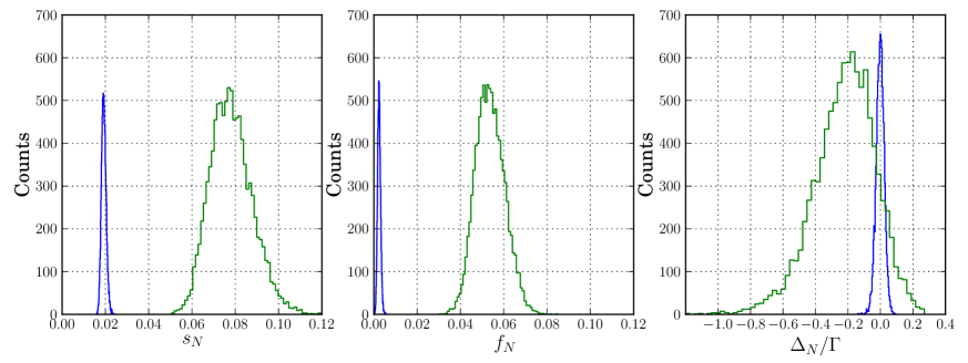
Figure 2: (color online) Distributions for values of $s_{N},f_{N}$ and $\Delta_{N}$ for $N=50$ atoms, plotted for $10000$ configurations for a size corresponding to $\sigma=10$ (blue curves) and $\sigma=2$ (green curves).

These values for $s_{\infty},f_{\infty}$ and $\Delta_{\infty}$ can be compared to numerical evaluation of the $s_{N},f_{N}$ and $\Delta_{N}$ for a finite number of atoms and a specific configuration. In Fig. 2 we show the distribution of these values for different sample size.

In our numerical simulations shown in Fig. 3 we observe strong configuration dependent fluctuations for the value of the collective Lamb shift. A precise comparison with our analytical expression, valid for large clouds, is thus cumbersome and did not allow us to validate precise predictions of the numerical factor in Eq. (42).

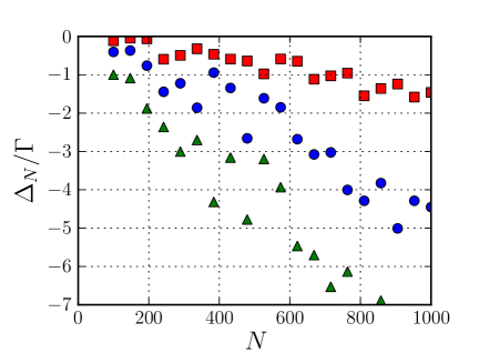
Figure 3: (color online) Collective Lamb shift vs atom number for $\sigma=1.6$ (green triangles) $\sigma=2$ (blue circles) and $\sigma=3$ (red squares).

Normalizing the radiation pressure force with respect to the single atom value, we obtain for large atomic samples,

$$\frac{\langle\hat{F}_{z}\rangle}{F_{1}}=\frac{4\Delta_{0}^{2}+\Gamma^{2}}{4(\Delta_{0}-\Delta_{N})^{2}+\Gamma^{2}(1+b_{0}/12)^{2}}\left[1+\frac{b_{0}}{24\sigma^{2}}\right]$$ (43)

Finally, from Eq.(29) we obtain the scattered intensity

$$I(\mathbf{r})=\left(\frac{I_{0}}{16\pi^{2}k_{0}^{2}r^{2}}\right)\left[\frac{\Gamma^{2}}{4(\Delta_{0}-\Delta_{N})^{2}+\Gamma^{2}(1+b_{0}/12)^{2}}\right]\left[N+N^{2}|S_{\infty}(\mathbf{k}_{s})|^{2}\right].$$ (44)

This expression of the scattered intensity illustrates the role of the shape of the atomic cloud for the modified emission diagram. The emission diagram of the TD state is shown in Fig. 4. It illustrates the strong forward emission by the cloud when its size exceeds a few optical wavelengths, reminiscent of Mie scattering, or more precisely of Rayleigh-Debye-Gans Hulst1957 . As we will discuss in the following section, a modified emission diagram yields a modified radiation pressure force, as the recoil of the scattered photon (partially) compensate the recoil effect at absorption.

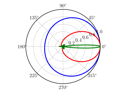
Figure 4: (color online) Emission diagram computed according to Eq. (29) for the Timed Dicke state $|+\rangle_{\mathbf{k}_{0}}$ with $N=40$ atoms : $\sigma=0.4$ (blue), $\sigma=1$ (red) , $\sigma=8$ (green).

V Heuristic approach

The result (36) can be interpreted heuristically considering the momentum balance in a given time interval $\delta t$ Dalibard . During $\delta t$, $N$ two-level atoms with positions $\mathbf{r}_{j}$ ($j=1,\dots,N$) do $\delta N$ florescence cycles, each time absorbing a photon with momentum $\hbar\mathbf{k}_{0}$ from the laser and emitting a photon with momentum $\hbar\mathbf{k}_{i}$ ($i=1,\dots,\delta N$) in a random direction $\mathbf{\Omega}_{i}$, with probability $P_{i,j}=P(\mathbf{\Omega}_{i},\mathbf{r}_{j})$. The momentum variation for the $j$th atom after $\delta N$ cycles is

$$\delta\mathbf{p}_{j}=(\hbar\mathbf{k}_{0})\delta N-\sum_{i=1}^{\delta N}(\hbar\mathbf{k}_{i})P_{i,j}.$$ (45)

For a single isolated atom the emission is isotropic and $P_{i,j}=1$, but for $N$ atoms the emission can be not isotropic depending on the atomic distribution. Also, the excitation could be not uniform if the phase front of the driving beam is getting distorted by the refractive index changes in the atomic cloud. Assuming for simplicity that the excitation is uniform over the entire atomic ensemble and neglecting phase distortion effects Gordon73 ; Ketterle05 , $\delta N$ will be the same for all the atoms and $|\mathbf{k}_{i}|=k_{0}$. Considering the momentum variation along the direction of the incident photon ($z$ axis), after averaging over the atoms

$$\delta p_{z}=\frac{1}{N}\sum_{j=1}^{N}\delta p_{j,z}=(\hbar k_{0})\delta N-(\hbar k_{0})\sum_{i=1}^{\delta N}P_{i}\cos\theta_{i}$$ (46)

where $P_{i}=(1/N)\sum_{j}P_{i,j}=P(\cos\theta_{i})$ is the emission probability along the angle $\theta_{i}$. Considering $\cos\theta_{i}$ and $\delta N$ as independent random variables, the statistical average of Eq.(46) is

$$\overline{\delta p_{z}}=(\hbar k_{0})\,\overline{\delta N}-(\hbar k_{0})\,\overline{\delta N}\cdot\overline{\cos\theta}$$ (47)

where we assumed $\overline{\sum_{i}\cos\theta_{i}}\approx\overline{\delta N}\cdot\overline{\cos\theta}$. Hence, the pressure force is

$$F_{z}=\frac{\overline{\delta p_{z}}}{\delta t}=(\hbar k_{0})\left(\frac{\overline{\delta N}}{\delta t}\right)\left[1-\overline{\cos\theta}\right]$$ (48)

Comparing with Eq.(36) we found the following correspondence

$$\left(\frac{\overline{\delta N}}{\delta t}\right)=\frac{\Omega_{0}^{2}\Gamma_{N}}{4(\Delta-\Delta_{N})^{2}+\Gamma_{N}^{2}}\quad,\quad\quad\overline{\cos\theta}=\frac{f_{N}}{s_{N}}$$ (49)

where $\Gamma_{N}=\Gamma Ns_{N}$. So, the scattering rate $(\overline{\delta N}/\delta t)$ is equal to the excitation probability, $\rho_{ee}=\Omega_{0}^{2}/[4(\Delta-\Delta_{N})^{2}+\Gamma_{N}^{2}]$, times the collective decay rate, $\Gamma_{N}$. The radiation pressure force (36) is equal to the momentum photon, $\hbar k_{0}$, multiplied by the scattering rate and by a geometrical factor $1-\overline{\cos\theta}$ taking into account the directionality of the scattered light. Cooperativity modifies both the scattering rate, enhancing the decay rate and shifting the resonance frequency, and the scattering direction. Small samples tend to radiate isotropically whereas extended samples radiate superradiantly in forward direction Courteille10 ; Prasad10 . These cooperative effects can be revealed measuring radiation pressure force by monitoring center-of-mass motion of large atomic clouds released by magneto-optical traps Bienaime10 ; Bender10 , and then identifying fast decay, shifts and modified emission diagrams described by Eqs.(36) and (44).

VI Product state

It has been noted that the same results obtained for a symmetric TD state could be obtained assuming a product state for $N$ atoms Eberly06 ; Friedberg10 (named also ‘Bloch state’ by some authors Friedberg07 ):

$$|\Psi(t)\rangle_{c}=\prod_{j=1}^{N}\left\{\alpha_{c}(t)|g_{j}\rangle+\beta_{c}(t)e^{i\mathbf{k}_{0}\cdot\mathbf{r}_{j}-i\Delta_{0}t}|e_{j}\rangle\right\},$$ (50)

where $\alpha_{c}(t)$ and $\beta_{c}(t)$ are the same for every atom, with $|\alpha_{c}(t)|^{2}+|\beta_{c}(t)|^{2}=1$. The ansatz of Eq. (50) assumes each $j$th atom driven into the excited state with equal probability $|\beta_{c}(t)|^{2}$ and phase $\phi_{j}=\mathbf{k}_{0}\cdot\mathbf{r}_{j}-\Delta_{0}t$. As it happens for the symmetric TD state (30), the driving field imposes a coherence in the photons emitted spontaneously by each atom, so that superradiance arises because the state is symmetric under exchange of particles Scully:LP . However, it is expected that the quantum statistic of the symmetric TD state will be quite different from that of the ’quasi-classical’ product state. Notice that for $|\beta_{c}|\ll 1$ the product state (50) can be written in the following form Friedberg07 ; Friedberg10b

$$|\Psi\rangle_{c} = \alpha_{c}^{N}|g\rangle+\alpha_{c}^{N-1}\beta_{c}\sum_{j}e^{i\mathbf{k}_{0}\cdot\mathbf{r}_{j}-i\Delta_{0}t}|j\rangle+\alpha_{c}^{N-2}\beta_{c}^{2}\sum_{j\neq m}e^{i\mathbf{k}_{0}\cdot(\mathbf{r}_{j}+\mathbf{r}_{m})-2i\Delta_{0}t}|j,m\rangle+\dots$$ (51)

where $|j,m\rangle=|g_{1},\dots,e_{j},\dots,e_{m},\dots,g_{N}\rangle$. Hence, the product state can be expanded in the symmetric TD states with $1$ to $N$ excited atoms. Only in the limits $\alpha_{c}\approx 1$ and $|\beta_{c}|\ll 1$ the product state reduces to the symmetric single-excited atom state $|\psi\rangle\approx|g\rangle+\beta_{c}\sqrt{N}|+\rangle_{\mathbf{k}_{0}}$ if only the first two terms of Eq. (51) are retained. The expectation values for the state (50) are $\langle\hat{\sigma}_{j}\rangle=\alpha_{c}^{*}\beta_{c}$ and $\langle\hat{\sigma}_{m}^{\dagger}\hat{\sigma}_{j}\rangle=|\alpha_{c}|^{2}|\beta_{c}|^{2}$, so for $\alpha_{c}\approx 1$ they coincide with those obtained from the symmetric TD state. Differences between the product and the symmetric TD states should appear when higher-order expectation values are observed, as for instance $\langle\hat{\sigma}_{j}\hat{\sigma}_{m}\rangle$, which is zero for the TD state and $\alpha^{*2}\beta_{j}\beta_{m}\approx\beta_{j}\beta_{m}$ for the product state. Notice that operator ordering produces different results in high-order expectation values if scattered photons or atomic forces are measured. These features and non classical effects studies in cooperative scattering by cold atoms will be the object of a future investigation.

VII Conclusion

In this paper, we have included a more precise kernel to evaluate the cooperative radiation pressure force on a cloud of two-level systems. The collective Lamb shift leads to a shift $\Delta_{N}$ of the resonance, which is proportional to the spatial density. As we have used a scalar model in this paper, near field and polarization effects are neglected. One thus needs to consider this shift with some scepticism as the numerical factor for this shift in a real system will be strongly modified by the vectorial nature of the light Friedberg . For dilute clouds, we recover previous results Bienaime10 , where these density effects are negligible. We also presented a simple model to estimate the radiation pressure force from the modified emission diagram and assuming coupling to the single photon superradiant (Timed Dicke) state Scully06 . This approach can be useful to estimate not only average forces but also fluctuations and dissipation. Finally, we noted that in the low intensity limit, the average result we derived for the cooperative radiation pressure force can be obtained either by assuming a driven Timed Dicke state or a product state Eberly06 ; Friedberg07 ; Friedberg10 , with no entanglement required. Looking for non classical features in cooperative scattering of light by a cloud of two-level system thus requires studies of higher orders either by using higher intensities or looking at correlations or fluctuations of the force.

VIII Acknowledgements

We acknowledge fruitful discussions with E. Akkermans, P. Courteille, M. Havey, I. Sokolov and stimulating presentations on this topic at the PQE 2011 conference.

Appendix A Evaluation of the integral kernel in Eq.(6)

Let’s consider the last term in Eq.(6) and pass to the continuous frequency approximation:

$$I(\mathbf{r}_{jm})=\sum_{\mathbf{k}}g_{k}^{2}e^{i\mathbf{k}\cdot\mathbf{r}_{jm}}\int_{0}^{t}dt^{\prime}\hat{\sigma}_{m}(t-t^{\prime})\,e^{-ic(k-k_{0})t^{\prime}}\rightarrow\frac{V_{ph}}{(2\pi)^{3}}\int d\mathbf{k}g_{k}^{2}e^{i\mathbf{k}\cdot\mathbf{r}_{jm}}\int_{0}^{t}dt^{\prime}\hat{\sigma}_{m}(t-t^{\prime})\,e^{-ic(k-k_{0})t^{\prime}}.$$ (52)

We exchange the integration order and introduce spherical coordinates, $d\mathbf{k}=dkk^{2}d\phi\,d\theta\sin\theta$. After integration of the angular part, we obtain

$$I(\mathbf{r}_{jm})=\frac{V_{ph}}{2\pi^{2}}\int_{0}^{t}dt^{\prime}\hat{\sigma}_{m}(t-t^{\prime})e^{ick_{0}t^{\prime}}\int_{0}^{\infty}dkk^{2}g_{k}^{2}\frac{\sin(kr_{jm})}{kr_{jm}}e^{-ickt^{\prime}}.$$ (53)

where $r_{jm}=|\mathbf{r}_{jm}|$. We approximate the $k$ integral as

$$\int_{0}^{\infty}dkk^{2}g_{k}^{2}\frac{\sin(kr_{jm})}{kr_{jm}}e^{-ickt^{\prime}}\approx\frac{k_{0}^{2}g_{k_{0}}^{2}}{2ik_{0}r_{jm}}\int_{-\infty}^{\infty}dk\left\{e^{-ick(t^{\prime}-r_{jm}/c)}-e^{-ick(t^{\prime}+r_{jm}/c)}\right\},$$ (54)

where we made the following approximations: a) we assumed the spectrum centered around $k\approx k_{0}$, so that $kg_{k}^{2}\approx k_{0}g_{k_{0}}^{2}$; b) we extended the lower integration value from $0$ to $-\infty$, since the relevant values of $k$ are around $k_{0}$. Using the expression above, we write

$$I(\mathbf{r}_{jm})=\frac{\Gamma}{2ik_{0}r_{jm}}\int_{0}^{t}dt^{\prime}\hat{\sigma}_{m}(t-t^{\prime})e^{ick_{0}t^{\prime}}\left\{\delta(t^{\prime}-r_{jm}/c)-\delta(t^{\prime}+r_{jm}/c)\right\}=\frac{\Gamma}{2}\,\frac{e^{ik_{0}r_{jm}}}{ik_{0}r_{jm}}\hat{\sigma}_{m}(t-r_{jm}/c).$$ (55)

where $\Gamma=V_{ph}k_{0}^{2}g_{k_{0}}^{2}/(\pi c)$. We observe that this approach does not require to assume the Markov approximation before solving the time integral, as in the standard approach Svi10 . On the contrary, this approach allows to obtain the retarded (or not local) kernel, which, when the ‘rapid transit approximation’ is assumed, i.e. $\hat{\sigma}_{m}(t-r_{jm}/c)\approx\hat{\sigma}_{m}(t)$, reduces to the exponential kernel of Eq.(8).

Appendix B Collective Lamb shift for a Gaussian distribution

Let consider Eq.(33) for a continuous distribution:

$$\Delta_{\infty} = -\frac{\Gamma N}{8\pi^{2}}\textrm{P}\int_{0}^{\infty}\frac{d\kappa\kappa^{3}}{\kappa-1}\int_{0}^{2\pi}d\phi\int_{0}^{\pi}d\theta\sin\theta\left|S_{\infty}(\kappa,\theta,\phi)\right|^{2}.$$ (56)

A spherical Gaussian distribution, $n(r)_{0}\exp(-r^{2}/2\sigma_{R}^{2})$, yields $S_{\infty}(\kappa,\theta,\phi)=\exp[-\sigma^{2}(\kappa^{2}+1-2\kappa\cos\theta)/2]$, where $\sigma=k_{0}\sigma_{R}$. Inserting it in eq.(56) we obtain

$$\Delta_{\infty} = -\frac{\Gamma N}{4\pi}\textrm{P}\int_{0}^{\infty}\frac{d\kappa\kappa^{3}}{\kappa-1}e^{-\sigma^{2}(\kappa^{2}+1)}\int_{0}^{\pi}d\theta\sin\theta e^{2\sigma^{2}\kappa\cos\theta}$$ (57)

$$= -\frac{\Gamma N}{8\pi\sigma^{2}}\textrm{P}\int_{0}^{\infty}\frac{d\kappa\kappa^{2}}{\kappa-1}\left[e^{-\sigma^{2}(\kappa-1)^{2}}-e^{-\sigma^{2}(\kappa^{2}+1)^{2}}\right]$$

$$= -\frac{\Gamma N}{8\pi\sigma^{2}}\textrm{P}\int_{0}^{\infty}d\kappa\left(\kappa+1+\frac{1}{\kappa-1}\right)\left[e^{-\sigma^{2}(\kappa-1)^{2}}-e^{-\sigma^{2}(\kappa+1)^{2}}\right]$$

$$= -\frac{\Gamma N}{8\pi\sigma^{2}}\textrm{P}\int_{-1}^{\infty}dx\left(2+x+\frac{1}{x}\right)\left[e^{-\sigma^{2}x^{2}}-e^{-\sigma^{2}(2+x)^{2}}\right].$$

For $\sigma\gg 1$ it is approximated by

$$\Delta_{\infty} \approx -\frac{\Gamma N}{8\pi\sigma^{2}}\textrm{P}\int_{-\infty}^{\infty}dx\left(2+\frac{1}{x}\right)e^{-\sigma^{2}x^{2}}\approx-\frac{\Gamma N}{4\sqrt{\pi}\sigma^{3}},$$ (58)

in agreement with the result of Friedberg and Manassah Friedberg10b .