YSO jets in the Galactic Plane from UWISH2:
I - MHO catalogue for Serpens and Aquila

Abstract

Jets and outflows from Young Stellar Objects (YSOs) are important signposts of currently ongoing star formation. In order to study these objects we are conducting an unbiased survey along the Galactic Plane in the 1-0 S(1) emission line of molecular hydrogen at 2.122 $\mu$m using the UK Infrared Telescope. In this paper we are focusing on a 33 square degree sized region in Serpens and Aquila (18^∘<l <30^∘; -1.5^∘<b <+1.5^∘).

We trace 131 jets and outflows from YSOs, which results in a 15 fold increase in the total number of known Molecular Hydrogen Outflows. Compared to this, the total integrated 1-0 S(1) flux of all objects just about doubles, since the known objects occupy the bright end of the flux distribution. Our completeness limit is 3 $\cdot$ 10^-18 W m^-2 with 70 % of the objects having fluxes of less than 10^-17 W m^-2.

Generally, the flows are associated with Giant Molecular Cloud complexes and have a scale height of 25 – 30 pc with respect to the Galactic Plane. We are able to assign potential source candidates to about half the objects. Typically, the flows are clustered in groups of 3 – 5 objects, within a radius of 5 pc. These groups are separated on average by about half a degree, and 2/3rd of the entire survey area is devoid of outflows. We find a large range of apparent outflow lengths from 4″ to 130″. If we assume a distance of 3 kpc, only 10 % of all outflows are of parsec scale. There is a 2.6 $\sigma$ over abundance of flow position angles roughly perpendicular to the Galactic Plane.

1 Introduction

The interstellar medium (ISM) in galaxies is radically influenced by star formation. Giant Molecular Clouds (GMCs) are heated and excited by outflows from protostars and radiation from high-mass young stellar objects (YSO). Changes in chemistry and probably the turbulent motion in GMCs are a result of star formation, especially massive star formation. Therefore, it is of great importance to understand the formation of stars.

Jets and outflows from YSOs are sign-posts of currently ongoing star formation (e.g. Bally et al. (1995); Eislöffel (2000); Froebrich & Scholz (2003); Davis et al. (2009)). Previous studies of star forming regions like the Orion A molecular ridge by Davis et al. (2009) and Stanke et al. (2002), DR 21/W 75 by Davis et al. (2007), as well as the Taurus-Auriga-Perseus clouds by Davis et al. (2008), have shown a large number of outflows from YSOs. However, there are a number of open questions which are still to be addressed. For example: Is a large number of jets and outflows a common occurrence in other star forming regions (low and high mass)? Is star formation triggered in infrequent bursts or is it an ongoing, multiple epoch process in each GMC? The presence of jets from YSOs is an indication of a young population and active accretion while the sparsity of them in regions with a sizeable population of reddened sources shows a more evolved region with a larger population of pre-main-sequence stars. The dynamical age of a protostellar outflow is 10 to 100-times less than the turbulent lifetime of a GMC. Therefore, the presence of a large number of outflows will be an indication of currently ongoing or multiple epochs of star formation.

Outflows from YSOs are also a direct tracer of mass accretion and ejection and can be used to estimate star formation efficiency from region to region. This is particularly the case in high mass star forming regions where the efficiency is grossly affected by existing massive young stars, which influence the environment via their hugely energetic winds and intense UV fluxes. Furthermore, in massive star forming regions, where young stars form in clusters and massive stars influence their lower-mass neighbours, photo-evaporation and ablation of protostellar disks can suppress accretion. As a result the mechanism that drives the jets and outflows is switched off. To what degree do these interactions affect accretion in YSOs?

The position of individual protostars can be detected from jets and outflows while their evolutionary stage (e.g. Class 0, Class I) is closely related to the brightness in H₂ emission (Caratti o Garatti et al., 2006). The mass infall/ejection history can be determined from jets since there is a correlation between the jet parameters, mass infall rates and accretion luminosities (Beck, 2007; Antoniucci et al., 2008).

Studies by Eislöffel et al. (1994) and Banerjee & Pudritz (2006) suggest that outflows are aligned parallel with the local magnetic field and perpendicular to the chains of cores. However, existing observations give mixed results without a definite answer (Anathpindika & Whitworth, 2008; Davis et al., 2009). Is there a correlation between the mass of the driving source and the orientation of the flow with respect to the cloud filament (i.e. are massive outflows more likely to be orthogonal to the filaments than flows from low mass stars)? Furthermore: What fraction of outflows and jets are collimated, and what fraction are parsec-scale in length? Is there a correlation between the median age of the embedded population and the mean flow length? Are outflows sufficient in numbers and energetic enough to account for the turbulent motions in GMCs?

In order to answer the above outlined questions we need to have a representative sample of jets and outflows from young stars which is free from selection effects. This will allow us to perform a statistically meaningful investigation of the dynamical processes associated with (massive) star formation. Therefore we are conducting an unbiased search for jets and outflows in the Galactic Plane using the UKIRT Wide Field Infrared Survey for H₂ (UWISH2 – Froebrich et al. (2011), hereafter F11). The data is taken in the H₂ 1-0 S(1) emission line at 2.122 $\mu$m, and thus highlights regions of shock excited molecular gas (T $\approx$ 2000 K, n${}_{\rm H_{2}}>$ 10³ cm^-3), as well as fluorecently excited material. Hence, it can be used to trace outflows and jets from embedded young stars.

In this project we focus our attention on the Serpens/Aquila region in the Galactic Plane, covered by UWISH2. In particular we investigate the area 18^∘<l <30^∘; -1.5^∘<b <+1.5^∘, which approximately covers 33 square degrees (see Fig. 1 for an overview of the region). It is the first continuous area of this size completed and covers about 20 % of the total UWISH2 area. Hence, it will allow us to obtain first but statistically significant results about the population of jets and outflows from young stars in the Galactic Plane.

In this paper we present our analysis of the above mentioned region. We focus on the detection of the jets and outflows, as well as their potential sources. We further analyse the spatial distribution of the discovered objects, their apparent lengths, position angles and fluxes. To convert apparent measurements (such as size) into physically meaningful measurements we need the distance. We assume that all outflows are at a distance of 3 kpc throughout the paper, since this turns out to be the most commonly measured distance for outflows in our sample. In our forthcoming paper (Ioannidis & Froebrich, in prep., Paper II) we will discuss in detail our distance measurement method of the individual jets and outflows. We will then determine in detail statistically corrected luminosity functions and length distributions of the jets and outflows and investigate their distribution in the Galactic Plane. Finally, in Ioannidis & Froebrich (in prep., Paper III) we will investigate the driving source properties as well as the environment (cloud structure, clustered and isolated star forming regions) the jets and outflows are in.

In Sect. 2 we discuss our data and analysis methods. We then present our results and discussion in Sect. 3, which includes the positions and distribution of outflows, the lengths and flux distributions as well as their orientation. We conclude our findings in Sect.4.

2 Data and Analysis

2.1 Near infrared UKIRT WFCAM data

We obtained our near infrared narrow band imaging data in the 1-0 S(1) line of H₂ using the Wide Field Camera (WFCAM - Casali et al. (2007)) at the United Kingdom Infrared Telescope (UKIRT). The camera consists of four Rockwell Hawaii-II (HgCdTe 2048 $\times$ 2048) arrays with a pixel scale of 0.4″. The 1-0 S(1) filter is centred at 2.122 $\mu$m with $\Delta\lambda$ = 0.021 $\mu$m. Our data is part of the UWISH2 survey (see F11 for details) and the H₂ images are taken with a per pixel integration time of 720 s under very good seeing conditions. The typical full width half maximum (fwhm) of the stellar point spread function is 0.7″, the 5 $\sigma$ point source detection limit is about 18 mag (in broad-band K) and the surface brightness limit is about 10^-19 W m^-2 arcsec^-2 when averaged over the typical seeing (F11). Our narrow band data were taken between 31st of July 2009 and 9th of September 2010.

Furthermore, we utilised the UK Infrared Deep Sky Survey (UKIDSS) data in the near infrared $JHK$ bands taken with the same telescope, same instrumental set-up and tiling as part of the Galactic Plane Survey (GPS, Lucas et al. (2008)) in order to perform the continuum subtraction (H₂-$K$) of our narrow band images and to generate three band colour images ($JHK$, $JH$H₂, $JK$H₂; see Sect.2.3). When compared to our narrow band data the NIR broad band data has very similar quality (fwhm and depth). Both data sets are taken typically about 2.5 to 4.0 years apart.

Data reduction and photometry for both NIR data sets are done by the Cambridge Astronomical Survey Unit (CASU). Reduced images and photometry tables are available via the Wide Field Astronomy Unit (WFAU). The basic data reduction procedures applied are described in Dye et al. (2006). Calibration (photometric as well astrometric) is performed using 2MASS (Skrutskie et al. (2006)) and the details are described in Hodgkin et al. (2009).

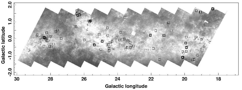
Figure 1: Positions of outflows (black squares) over plotted on a relative extinction map (grey scale image) based on near infrared colour excess in GPS data. Please see text for details on the background map.

2.2 Difference Images

In order to reveal mutually exclusive emission line regions associated with H₂ jets and outflows (or other H₂ emitters), the H₂ narrow band images have been continuum-subtracted using the $K$-band images from the GPS. Note that we are working with images about 13.3′ $\times$ 13.3′ in size throughout the project, since these are the images delivered by CASU. Every set of images (H₂, $K$) is aligned based on their World Coordinate System (WCS). Photometry is performed to determine the mean fwhm of each image.

To compensate for the different seeing conditions in both images and to enhance the signal to noise ratio in the difference images we Gaussian smoothed both images before the continuum subtraction. The image with the worse seeing (image $b$) is smoothed using a Gaussian with a fwhm of $r_{s}^{b}$ = 0.4″. The image with the better seeing (image $a$) is smoothed with a Gaussian of a larger fwhm ($r_{s}^{a}$), which we calculate as:

$$r_{s}^{a}=\sqrt{(fwhm^{b})^{2}-(fwhm^{a})^{2}+(r_{s}^{b})^{2}}$$

where $fwhm^{a}$ is the mean fwhm of image $a$ and $fwhm^{b}$ is the mean fwhm of image $b$. Typically the seeing in both images is very similar and the smoothing radii $r_{s}^{a}$ and $r_{s}^{b}$ are thus not very different.

In order to completely remove continuum sources such as stars in the difference images, the $K$-band images need to be scaled. Since the scaling factor $sc$ depends on the foreground extinction to the stars, we expect this to vary significantly across images taken in the Galactic Plane. We thus use a position dependent scaling factor $sc(x,y)$ (’scaling image’) for the continuum subtraction.

For this purpose we determine the mean scale factor for all stars in small sub-regions (10″$\times$ 10″). Before applying the scaling image to the K-band it is smoothed with a radius of 30″. Thus, we trace as much structure of the foreground extinction as possible while ensuring a sufficient signal to noise of the scale factor.

The final difference images are then created as:

$${\rm Difference}_{H_{2}-K}=H_{2}-K*sc$$

Due to the Gaussian smoothing to adapt the stellar fwhm, the resulting difference images have a higher signal to noise than the original H₂ and $K$ images. While most of the non saturated stars are not present the H₂ emission features are preserved. We note that the difference images are only used for the purpose of detection of jets and outflows from protostars (see Subsection 2.4) and not for photometry.

2.3 NIR Colour images

The search for H₂ emission features (as described in Section 2.4) is mainly based on the H₂-$K$ difference images. However, the verification that the observed feature is indeed a jet or outflow from a young stellar object is greatly facilitated by the additional use of near infrared colour composite images obtainable from our data sets. These images are also extremely useful to identify potential driving sources for the discovered jets and outflows.

We thus created full resolution near infrared $JHK$, $JH$H₂ and $JK$H₂ colour composites for every image. Each of the colour combinations enhances different aspects of the spectrum and therefore makes it easier to visually detect and/or verify objects of interest. More specifically, the $JK$H₂ images can be used to detect pure H₂ emission regions. Since the H₂ and $K$ images have been taken at two different epochs, very ’red’ or very ’green’ objects can be identified as $K$-band variable stars in the $JK$H₂ composites. In contrast, the $JHK$ and $JH$H₂ images can be used to detect objects with $K$-band excess emission, in other words candidate young stellar objects.

2.4 Outflow detection

Our aim to investigate an unbiased sample of jets and outflows from young stars in the Galactic Plane cannot just be achieved by performing an unbiased survey. We also need to take great care not to introduce any detection bias when identifying the objects in our data. Thus, we follow the strategy described below to find all potential jet and outflow candidates.

All H₂-$K$ difference images have been visually inspected for extended H₂ emission features in full resolution. The order of inspection was completely random to avoid the introduction of biases due to our search pattern. The original search has been performed by just one of us. However, the subsequent cleaning of this input catalogue (see below) has been done by two people.

Every detected emission feature that has been identified in the H₂-$K$ difference images at first has been confirmed in the corresponding H₂ image to avoid the inclusion of image artefacts. We then checked it against the full resolution $JK$H₂ colour composite of the region (such as the one shown in Fig. 2). Thus, any object that could potentially be an image artefact has been removed from the source list.

Finally, we need to clean the remaining objects from real emission contaminants. These include e.g. Planetary Nebulae (PN), Supernova Remnants (SNR) and fluorescently excited regions such as edges of molecular clouds, HII regions and areas around young embedded clusters with massive stars. Planetary Nebulae can usually be identified by their visual appearance. In the case of SN shocks and fluorescently excited cloud edges this is more complicated, as they can mimic shocks from jets and outflows. We searched the SIMBAD database for known SNRs near to our identified objects. Any potential feature detected near such known SNRs has been excluded from our list. We inspected regions with (obviously) fluorescently excited cloud edges very carefully and excluded any object that potentially was not a jet/outflow feature.

The resulting list of H₂ emission line objects is thus complete up to the survey detection limit, contains (almost) no false positives and is unbiased.

2.5 Driving sources of outflows

One vital task in order to understand the properties of the detected jets and outflows (e.g. the length distribution) is the identification of their potential driving sources. We utilise a number of published catalogues of YSOs as well as mid and far infrared source lists for this purpose. These include the catalogue of YSOs compiled by Robitaille et al. (2008) from the Spitzer GLIMPSE survey (Churchwell et al., 2009), detections in the AKARI/IRC mid-infrared all-sky survey bright source catalogue (Ishihara et al., 2010; Yamamura et al., 2009), detections in the IRAS Point and Faint Source Catalogue (Moshir, 1989, 1991) and detections in the Bolocam Galactic Plane Survey (Aguirre et al., 2011), which all cover our entire survey field. Additionally we used $K$-band excess sources identified from $JHK$ detected objects in the UKIDSS GPS, as well as $K$-band variable sources identified in the H₂-$K$ difference images as potential driving source candidates.

To decide on the most likely source for each H₂ feature, we over-plot all potential source candidates over the H₂-$K$ difference images. Based on the vicinity of source candidates and H₂ emission, the alignment of a number of emission knots with a potential source, or the shape of bow-shock like features we grouped the H₂ emission objects into outflows and assigned one MHO number to each of them, following the procedure outlined in Davis et al. (2010). Figure 2 shows MHO 2204 as an example of a detected jet with a potential source candidate.

There are cases with several potential source candidates. If it is impossible to decide on one specific one we consider all possibilities. In cases where non of the above mentioned catalogues allowed us to find a potential source for an H₂ feature, we additionally searched the SIMBAD database for other indicators of YSO outflow sources, such as masers and (sub)-mm sources. Finally, if there are several source candidates which apparently are the same object (such as an IRAS, Bolocam and Glimpse detection at roughly the same coordinates), we use as the source position and identifier the object in the survey with the highest spatial resolution. There are a number of cases where we clearly detect a small, bipolar and symmetric jet but no object has been detected in any survey at the suspected source position. In these cases we assume the source to be situated between the H₂ features on the flow axis, and it is given the identifier ’Noname’. Note, that MHO 2444 would be one of these objects, if it had not had deep JCMT data from Di Francesco et al. (2008).

2.6 Photometry

After the detection of the H₂ emission features we have to measure their fluxes. This is straight forward, since our H₂ images have been flux calibrated by CASU.

We define apertures around each emission feature in the H₂ images. Great care is taken that continuum sources (such as fore or background stars at the same line of sight) are not included in the apertures. We also ensure that the apertures contain as little area as possible that seems to be free of emission in order not to add noise. Simultaneously, we use for each H₂ feature a nearby sky-aperture that is completely emission free and defines the local sky level (see Fig. 2 for an example of the apertures used in the photometry of MHO 2204). We then measure the number of counts in the H₂ feature, corrected for the local background level and repeat that measurement, using identical aperture positions, in the scaled (using $sc(x,y)$, see Sect. 2.2 above) $K$-band image to correct for the continuum contained in the narrow band data.

The background- and continuum-corrected H₂ counts for each emission feature are then converted into physical flux units ($W/m^{2}$) using the flux zero points provided by CASU. The final flux values for the H₂ emission in the 1-0 S(1) line (summed up over all knots in each MHO) are shown in Table LABEL:outflow_table in the Appendix.

Uncertainties in the photometry are based on the variation of the local background level in the H₂ and $K$-band images and the choice of the exact position of the apertures enclosing the H₂ emission regions. Typical uncertainties of the measured fluxes are discussed in Sect. 3.5.

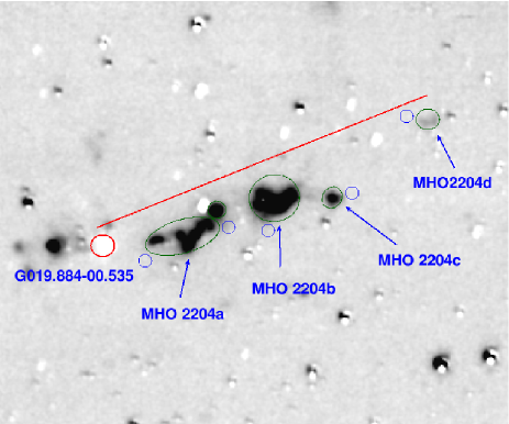
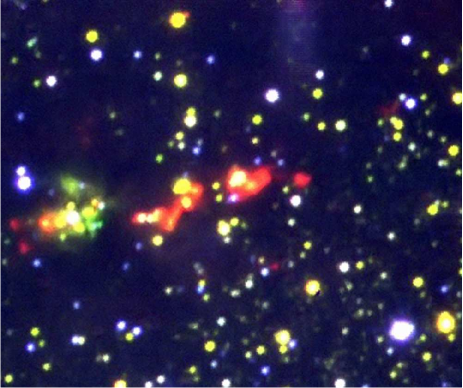
Figure 2: Left: Grey scale representation of the H₂-$K$ difference image of MHO 2204. The green ellipses indicate the apertures used to enclose the H₂ flux, while the blue apertures represent the nearby sky. The solid line indicates the direction of the flow. Right: JKH₂ color composite of the same region. Both images are 95″$\times$ 66″ in size, North is to the top and East to the left.

3 Results and Discussion

We have detected a total of 131 molecular hydrogen outflows from YSOs in our survey field of 33 square degrees. Out of these, 121 (92 %) objects are new discoveries. Of the ten already known outflows, two have been recently identified by Lee et al. (2011 in preparation) using UWISH2 data as well. Thus, 94 % of our outflows are newly discovered in our data set. Hence, in the field investigated here, the UWISH2 data increased the number of known molecular hydrogen outflows by a factor of 15.

In Table LABEL:outflow_table in the Appendix we list the assigned MHO numbers, positions, fluxes, apparent lengths, position angles, source candidates and their positions. In Table LABEL:images_table we show H₂-$K$ images of each MHO and give a brief description of its morphology and potential sources. We note that there is a difference between the number of outflows (131) and the number of MHOs (134). The reason for this is that some of the already assigned MHO numbers are part of the same outflow. More specifically MHO 2206, MHO 2207 and MHO 2208 are part of the same outflow. Similarly, the bow shock MHO 2212 is part of the same flow as MHO 2201. In cases like these we treat all MHOs as one outflow. All objects in Table LABEL:outflow_table that are part of an outflow containing several MHOs are marked with an asterisk.

3.1 Spatial distribution and clustering of outflows

We show the positions of all detected outflows in our field in Fig. 1. The grey-scale background map in this figure is a relative extinction map based on median near infrared colour excess (e.g. Rowles & Froebrich (2009)) determined from UKIDSS GPS data (Lucas et al. (2008)). Note that some regions in the map have small A_V off-sets. This is caused by known, minor photometric calibration issues of the GPS data which will be corrected in future data releases. Since we are not using the actual A_V values in the paper, this is a pure ’cosmetic’ issue.

As expected, the outflows are mainly located in areas with high extinction. Their overall distribution hence follows nicely the giant molecular cloud complexes visible in the A_V map. Only a small number of objects is not situated within dense clouds. However, there are numerous areas of high extinction where no outflows have been detected. In Paper III we will investigate in detail if there is an A_V threshold for the detection of molecular hydrogen flows, and which fraction of high column density clouds does not show signs of on-going star formation in the form of jets and outflows.

Histograms of the outflow positions along and across the Galactic Plane are shown in Fig. 3. As one can also see in Fig. 1, there is a non homogeneous distribution along the Plane, with peaks at $l$ = 20^∘ and $l$ = 25^∘ and a minimum around $l$ = 23^∘. This indicates the concentration of outflows to specific areas i.e. the giant molecular cloud complexes. The latitude distribution shows a Gaussian like distribution with a width of about one degree. Its centre is shifted to about $b$ = -0.25^∘ hinting that the main cloud complexes in this part of the Galactic Plane are at negative latitudes. If we assume a distance of 3 kpc for the outflows, the width of the distribution corresponds to a scale height of about 25-30 pc. This is very similar to values for young stellar clusters (55 pc, (Friel, 1995)) and OB stars (30 – 50 pc, (Reed, 2000; Elias et al., 2006)), but significantly smaller than the about 125 pc found for the dust at the solar galactocentric distance (e.g. Drimmel et al. (2003); Marshall et al. (2006)). The prominent increase of the number of objects at $b$ = 1.5^∘ (right panel of Fig. 3) is caused by a number of higher latitude clouds in particular at $l$ = 26.5^∘ (see also Fig. 1).

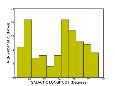
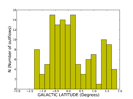
Figure 3: Histogram of the positions of the detected outflows along (left panel) and across (right panel) the Galactic Plane.

We have investigated the clustering of the detected outflows by means of nearest neighbour distance (NND) distributions. Hence, we calculated the distance to the N^th nearest neighbour for all outflows in our sample and determined a histogram to analyse these distance distributions. The 1^st, 2^nd and 3^rd NNDs all show a sharp peak at small separations, indicating that the flows are typically found in close proximity to each other. This peak almost disappears in the 4^th NND distribution and is certainly gone in the 5^th NND distribution, where it is replaced by a wider peak at about 20-30′ separation.

Thus, we find that the outflows typically occur in groups with a few (3-5) members. The size of these groups is about 6′  (a typical value for the 3^rd NND), which corresponds to about 5 pc if we assume all objects are at a distance of 3 kpc. This size is clearly larger than the typical embedded cluster (about 1 pc or slightly smaller; e.g. Lada & Lada (2003)) and smaller than typical nearby GMCs such as Taurus and Orion. Thus, currently ongoing star formation occurs in those 5 pc sized regions within GMCs and is not necessarily confined to embedded clusters.

The groups of outflows are separated by about half a degree on the sky from each other. Given the number of members in these groups, the average group separation, the total number of objects and the field size, we can estimate that about two thirds of the survey area are more or less devoid of molecular hydrogen emission line objects, a fact supported by the distribution shown in Fig. 1.

3.2 Driving source candidates

We have been able to assign driving source candidates, as described in Sect. 2.5, to 68 of our 131 molecular hydrogen outflows. This corresponds to just over half the objects. Overall, 75 source candidates have been identified, since some outflows have more than one probable driving source. A complete list of the outflow driving source candidates is presented in Table LABEL:outflow_table in the Appendix.

We find that typically brighter MHOs (according to their integrated 1-0 S(1) flux, see Sect. 3.5 below) are more likely to have a source candidate assigned to them. In particular the average flux of MHOs with an assigned source candidate is almost five times higher than for MHOs without source candidate. For the median fluxes this ratio, however, is lower by a factor of three. In a future paper we will investigate if this is a pure selection effect. It could simply be that bright MHOs are close-by and hence their sources are easier to detect. On the other hand, bright MHOs could be intrinsically luminous and thus be driven by brighter, easier to detect sources.

3.3 Apparent outflow lengths

For all outflows with assigned source candidate(s) we have measured the apparent length(s). A histogram of the resulting lengths distribution is shown in Fig. 4. The light grey bars represent all the outflows (68), while the dark grey areas represent the already known objects (9). Note that the lengths are not corrected for the unknown inclination angles or the potential detection of just parts of the outflow. For single sided flows the lengths correspond to the separation of the source and the most distant H₂ feature, while for bipolar flows the lengths correspond to the total length of the flow, a procedure also adopted in other surveys (Stanke et al., 2002). The known flows do not occupy a special part of the diagram, but rather represent a random sub-sample. Note that in cases of several source candidates for an outflow, we plot the distance corresponding to the most likely source. The distribution will not change significantly if we plot any other lengths.

There is a large range of apparent outflow lengths (from 4″ to 130″) and a strong decrease of the number of outflows with increasing length. Of the 68 outflows, more than 60 % have an apparent length of less than 30″ (or less than 0.4 pc if we assume a distance of 3 kpc). This is in agreement with the distribution of lengths found by Davis et al. (2009) and Stanke et al. (2002) along the Orion A molecular ridge and Davis et al. (2008) in Taurus-Auriga-Perseus (NGC 1333, L 1455, L 1448 and B 1). Only 10 % of all outflows have a length of more than 1 pc (if they are at 3 kpc). In Paper II we will discuss the physical outflow length distribution in parsec after considering the individual distances to the objects. Note that the observed distribution does not agree with a randomly orientated sample of flows which all have the same length.

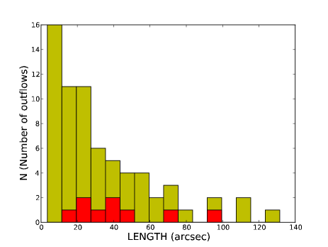
Figure 4: Histogram of the apparent outflow lengths. The light grey areas show all outflows, while the dark grey areas represent the known objects. In case there are several source candidates for one flow, the length corresponding to the most likely source is plotted. Note that an apparent length of 60″corresponds to about 0.9 pc for the assumed distance of 3 kpc.

3.4 Outflow position angles

Previous studies (e.g. Mouschovias (1976)) suggested that clouds collapse along magnetic field lines to form elongated, clumpy filaments from which chains of protostars are born. Furthermore, the associated outflows are aligned parallel with the local magnetic field and perpendicular to the chains of cores (Banerjee & Pudritz, 2006). Our sample is ideal to study the relation between cores, filaments and outflows because of the large sample of flows that are distributed over a considerable number of molecular clouds. We hence determined the outflow position angles and list them in Table LABEL:outflow_table in the Appendix.

A histogram of the position angles is shown in Fig. 5, using a bin-size of 30 degrees. The plot shows that a large fraction of outflows has a homogeneous distribution of position angles, with five of the six bins occupied by 11.2 objects on average. However, at angles between 120^∘ and 150^∘ one can identify an over abundance of outflows. There are 20 outflows in this bin, which corresponds to a 2.6$\sigma$ deviation from the average of the other bins. We performed a Kolmogorov-Smirnov test to determine the probability that the observed position angle distribution is identical to a homogeneously distributed sample. For outflows with two potential sources, and hence two possible position angles, each angle was weighted by half; if there are three sources the weight for each angle was one third. We find a probability of just 10 % that our objects are drawn from a homogeneously distributed sample.

We further investigated if there is a trend of objects with a particular range of position angles with sky position. Nothing could be found. The objects falling into a particular bin in the position angle histogram are distributed completely homogeneously amongst the entire sample.

The Galactic plane has an inclination of about 64 degrees with respect to the ecliptic in our survey area. Thus, the peak in the position angle histogram between 120^∘ and 150^∘ indicates that there is a 2.6$\sigma$ over abundance of outflows orientated almost (PA = 20^∘ with respect to Galactic North) perpendicular to the Galactic Plane. It is therefore possible that our measured flow position angles are influenced by the large scale cloud structure. Previous studies of the Orion A molecular cloud by Davis et al. (2009) and Stanke et al. (2002) and in Taurus-Auriga-Perseus by Davis et al. (2008) have shown a homogeneous distribution with no significant trends in the orientation of outflows. However, studies of DR 21/W 75 by Davis et al. (2007) have shown that flows (in particular massive ones) are orthogonal to some degree to the molecular ridge. In Paper III we will analyse this distribution in more detail. We will measure, if possible, the orientation of the outflows with respect to its parental cloud filament, to verify or disprove the above findings.

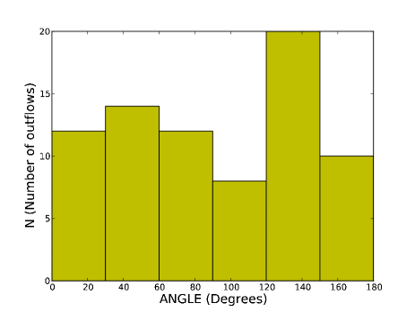
Figure 5: Histogram of the distribution of position angles from the detected outflows in 30 degrees bins. The distribution shows a 2.6 $sigma$ over abundance of flows with position angles between $l$ = 120^∘ and $l$ = 150^∘, or an orientation roughly perpendicular to the Galactic Plane.

3.5 Outflow flux distribution

The measured integrated 1-0 S(1) fluxes of the outflows are listed in Table LABEL:outflow_table in the Appendix. Figure 6 shows a histogram of this flux distribution. The light grey areas include all the outflows while the dark grey areas are the already known objects. Clearly, the known outflows dominate the bright end of the distribution and all but one are brighter than 10^-17 W m^-2. In particular, about 60 % of the integrated flux in the 1-0 S(1) line of molecular hydrogen can be attributed to already known MHOs. Thus, our survey just about doubles the known integrated 1-0 S(1) flux from jets and outflows in the survey area, in contrast to the 15 fold increase in total outflow numbers.

In general we find a sharp rise of the number of MHOs with decreasing integrated flux. More than 70 % of the MHOs have an integrated flux of less than 10^-17 W m^-2. The maximum number of MHOs occurs at about 3 $\cdot$ 10^-18 W m^-2 which corresponds to about 10^-3 solar luminosities in the 1-0 S(1) line of H₂ at our assumed distance of 3 kpc. We hence conclude that this flux is the completeness limit for outflows detected in our survey. There are, however, a number of objects with a significantly smaller integrated flux, indicating that the actual detection limit for 1-0 S(1) fluxes is lower than even 10^-18 W m^-2 in some regions (most likely dark clouds devoid of fore/background stars). This is also supported by fact that many of the outflows with a small overall integrated flux consist of only one emission line feature,

For each of the integrated fluxes we list the photometric uncertainties in Table LABEL:outflow_table. Typical uncertainties of the measured fluxes are of the order of 10 %. For bright objects they are significantly smaller. Wherever the integrated flux is very low and the variation of the local background level is high we only determine an upper flux limit.

How the measured integrated flux distribution converts into a statistically corrected luminosity distribution will be discussed in a forthcoming paper (Paper II).

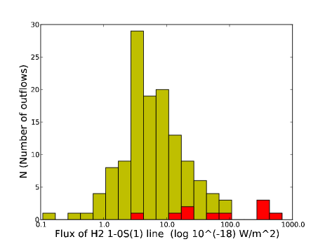
Figure 6: Histogram of integrated 1-0 S(1) fluxes (in logarithmic units) for the detected outflows. The light grey areas include all outflows while the dark grey areas represent the already known MHOs. Our completeness limit is about 3 $\cdot$ 10^-18 W m^-2.

4 Conclusions

In order to investigate the dynamical component of the star formation process we perform an unbiased search for jets and outflows from YSOs along the Galactic Plane. Our data has been taken as part of the UWISH2 survey (F11). It uses as a tracer the 1-0 S(1) emission line of H₂, and here we focus our attention on a continuous 33 square degree sized region (18^∘<l <30^∘; -1.5^∘<b <+1.5^∘) in Serpens and Aquila.

We identify 131 outflows from YSOs from which 94 % (123 objects) are new discoveries in our data set. Therefore, our survey has increased the number of known molecular hydrogen outflows by a factor of 15 in the area investigated.

We find a flux completeness limit for our outflow detection of 3 $\cdot$ 10^-18 W m^-2, with 70 % of the objects showing fluxes of 10^-17 W m^-2 or less. Typically, the already known outflows occupy the bright end of the flux distribution. Our survey thus increases the known integrated 1-0 S(1) H₂ flux from jets and outflows only by a factor of two, compared to the large increase in the total number of flows.

The overall spatial distribution of the detected outflows shows that they follow the GMC complexes in the Galactic Plane. Only a small number of objects is not situated within dense clouds. However, there are large areas with high extinction where no outflows have been detected. Overall, about 2/3rd of the survey area is more or less completely devoid of jets and outflows. We further find that the flows typically occur in groups of 3 – 5 members with a size of about 5 pc (at our assumed distance of 3 kpc). These groups are typically separated by about half a degree on the sky.

The distribution of flows perpendicular to the Galactic Plane shows a Gaussian like distribution with a width of about 25 – 30 pc (at our assumed distance of 3 kpc), similar to values for young stellar clusters and OB stars.

We are able to assign possible driving sources to about 50 % of the outflows. Brighter MHOs are more likely to have a source candidate assigned to them.

We measure the apparent outflow length for outflows with assigned driving sources. There is a wide range of lengths from 4″ to 130″ and a strong decrease of the number of flows with increasing length. More than 60 % of the outflows have an apparent length of less than 30″  (or less than 0.4 pc if we assume a distance of 3 kpc) while parsec-scale outflows are not common. Only 10 % of all outflows would have a length of greater than 1 pc at our assumed distance.

The position angle distribution of flows with assigned source shows an 2.6 $\sigma$ over-abundance at angles between 120^∘ and 150^∘.

Appendix A MHO Table

Table 1: Summary table of the MHO properties. The table lists the MHO number, Right Ascension and Declination (J2000), the integrated 1-0 S(1) flux and its uncertainty, the apparent length, the position angle, the source candidate(s) and its position(s). In cases where several MHOs belong to the same outflow, the MHO number is labelled with an asterisk. If the flux is an upper limit, no flux errors are given. Only for objects with a source candidate, we determined the apparent length and the position angle. Flow lengths are end-to-end for bipolar outflows or source-to-end for single sided flows. Source names correspond to the catalogue entries the source was taken from. These are either coordinate based, SIMBAD names, UKIDSS GPS IDs (12 digit numbers), or AKARI IDs (7 digit numbers). Sources labelled ’Noname’ are objects where it is assumed that there is a driving source at the listed position, however, non of the catalogues used shows a detection of the object. Please see the main text for details on the values in the table.

MHO	RA	DEC	F[1-0 S(1)]	Flux error	length	position angle	possible	source RA	source DEC
	(J2000)	(J2000)	[10E-18 W/m2]	[10E-18 W/m2]	(arcsec)	(degrees)	source	(J2000)	(J2000)
MHO 2201*	18:17:57.7	-12:07:19	379.119	37.885	73	132	IRAS 18151-1208	18:17:57.9	-12:07:20
MHO 2202	18:17:57.2	-12:07:30	77.481	5.632	21	32	IRAS 18151-1208	18:17:57.9	-12:07:20
MHO 2203	18:29:16.6	-11:50:17	278.893	19.586	42	67	G019.884-00.535	18:29:14.7	-11:50:24
MHO 2204	18:29:13.0	-11:50:16	509.659	42.892	50	116	G019.884-00.535	18:29:14.7	-11:50:24
MHO 2205	18:29:16.9	-11:49:54	58.429	3.918	-	29	-	-	-
MHO 2206*	18:34:22.7	-05:59:59	286.000	18.607	93	131	IRAS 18316-0602	18:34:20.9	-05:59:42
MHO 2207*	18:34:20.5	-05:59:38	9.664	1.027	*	*	*	*	*
MHO 2208*	18:34:18.4	-05:59:07	8.720	0.609	*	*	*	*	*
MHO 2209	18:34:18.8	-05:59:25	25.340	1.982	26	137	438649130203	18:34:20.0	-05:59:46
MHO 2210	18:34:21.3	-06:00:12	20.150	1.260	40	168	IRAS 18316-0602	18:34:20.9	-05:59:42
MHO 2212*	18:17:55.4	-12:06:42	26.363	1.926	-	-	-	-	-
MHO 2244	18:25:44.8	-12:22:46	3.005	0.217	35	160	3329252	18:25:44.7	-12:22:34
MHO 2245	18:29:14.8	-11:50:08	12.587	0.733	18	7	G019.884-00.535	18:29:14.7	-11:50:24
MHO 2246	18:29:12.7	-11:50:31	7.588	1.385	10	55	G019.8810-00.5300	18:29:13.3	-11:50:25
MHO 2247	18:26:58.9	-11:31:47	19.772	9.532	70	45	G019.896+00.103	18:26:57.6	-11:31:58
MHO 2248	18:29:12.3	-11:47:53	3.800	2.065	26	88	438521940668	18:29:13.2	-11:47:51
MHO 2249	18:30:04.6	-11:55:34	3.669	0.213	95	95	G019.9122-00.7799	18:30:11.1	-11:55:42
					64	145	3318624	18:30:06.9	-11:56:28
MHO 2250	18:28:18.9	-11:39:28	8.288	0.539	29	133	G019.9357-00.2558	18:28:19.9	-11:39:52
MHO 2251	18:28:19.1	-11:40:39	3.033	0.427	4	130	438521818214	18:28:18.9	-11:40:36
MHO 2252	18:25:22.8	-12:54:52	2.406	0.229	8.5	19	3349808	18:25:22.7	-12:55:00
MHO 2253	18:25:54.7	-12:01:59	10.497	0.640	-	-	-	-	-
MHO 2254	18:27:12.6	-10:33:57	9.463	0.543	54	44	3054756	18:27:15.2	-10:33:20
MHO 2255	18:29:10.9	-10:18:07	1.058	0.279	10	66	G021.2369+00.1940	18:29:10.2	-10:18:11
MHO 2256	18:29:09.3	-10:18:24	3.435	0.277	9	68	Noname	18:29:09.3	-10:18:24
MHO 2257	18:29:08.5	-10:18:54	4.862	0.751	18	9	G021.2248+00.1953	18:29:08.6	-10:18:48
MHO 2258	18:32:17.1	-10:34:19	4.044	0.428	-	-	-	-	-
MHO 2259	18:29:03.7	-09:44:13	7.424	0.867	-	-	-	-	-
MHO 2260	18:30:35.0	-09:34:45	22.339	1.768	25	78	438379615372	18:30:33.5	-09:34:49
MHO 2261	18:30:33.4	-09:35:07	62.588	7.425	72	29	438379615655	18:30:34.0	-09:34:52
MHO 2262	18:33:20.1	-07:55:44	15.495	Upper Limit	18	142	3058500	18:33:19.4	-07:55:32
MHO 2263	18:34:20.7	-08:17:51	6.439	1.059	23	166	G023.6008-00.0147	18:34:21.1	-08:18:13
MHO 2264	18:34:23.4	-08:18:07	15.185	1.073	18	40	3057470	18:34:22.7	-08:18:20
MHO 2265	18:33:11.6	-10:06:15	3.983	0.469	18	100	438517255051	18:33:12.7	-10:06:18
					5	136	438517254983	18:33:11.4	-10:06:12
MHO 2266	18:30:41.7	-09:34:58	5.976	0.509	28	0	G022.0535+00.1980	18:30:41.6	-09:34:40
MHO 2267	18:34:51.3	-08:57:51	3.236	0.246	-	-	-	-	-
MHO 2268	18:34:21.3	-08:33:24	0.111	Upper Limit	-	-	-	-	-
MHO 2269	18:34:31.0	-08:42:48	32.477	5.279	60	77	JCMTSE J183431.5-084250	18:34:31.4	-08:42:46
MHO 2270	18:35:28.5	-08:51:43	1.148	0.099	8	158	Noname	18:35:28.3	-08:51:36
MHO 2271	18:35:31.7	-08:52:17	6.578	0.465	-	-	-	-	-
MHO 2272	18:35:51.3	-08:41:13	3.822	0.239	4	45	G023.4319-00.5212	18:35:51.4	-08:41:10
MHO 2273	18:35:07.0	-08:05:47	2.535	0.338	-	-	-	-	-
MHO 2274	18:36:41.1	-07:39:20	17.829	2.088	66	0	438511042387	18:36:40.9	-07:39:02
MHO 2275	18:36:13.0	-07:42:40	17.181	2.264	-	-	-	-	-
MHO 2276	18:35:22.9	-07:19:17	2.777	0.165	-	-	-	-	-
MHO 2277	18:33:51.0	-07:06:13	24.144	1.847	-	134	-	-	-
MHO 2278	18:36:09.2	-06:50:07	13.823	0.936	20	36	3338999	18:36:09.9	-06:49:53
MHO 2279	18:38:51.9	-06:51:01	3.023	0.215	5	117	438745913239	18:38:52.1	-06:51:02
MHO 2280	18:38:55.4	-06:52:37	6.770	1.073	-	-	-	-	-
MHO 2281	18:38:57.3	-06:53:15	6.350	0.620	-	-	-	-	-
MHO 2282	18:36:56.6	-06:48:24	3.561	0.233	-	-	-	-	-
MHO 2283	18:37:21.9	-07:31:56	2.511	0.242	20	39	438368016438	18:37:22.7	-07:31:41
					34	103	G024.6280-00.3175	18:37:20.7	-07:31:51
MHO 2284	18:37:22.9	-07:31:58	3.745	0.674	18	170	438368016438	18:37:22.7	-07:31:41
					20	12	G024.635-00.325	18:37:23.3	-07:31:40
					34	103	G024.6280-00.3175	18:37:20.7	-07:31:51
MHO 2285	18:37:22.1	-07:32:14	2.482	0.183	33	14	438368016438	18:37:22.7	-07:31:41
					33	139	G024.6280-00.3175	18:37:20.7	-07:31:51
					38	25	G024.635-00.325	18:37:23.3	-07:31:40
MHO 2286	18:37:22.4	-07:37:08	13.093	1.088	-	126	-	-	-
MHO 2287	18:37:12.3	-07:11:26	3.239	0.192	-	-	-	-	-
MHO 2288	18:37:21.6	-07:11:38	10.087	0.622	-	-	-	-	-
MHO 2289	18:37:21.7	-07:11:46	3.036	0.182	-	-	-	-	-
MHO 2290	18:37:19.8	-07:11:44	12.735	1.197	27	140	G024.926-00.157	18:37:19.4	-07:11:35
MHO 2291	18:39:11.3	-07:20:09	38.832	3.432	112	147	438366899733	18:39:11.8	-07:20:22
MHO 2292	18:38:59.6	-06:12:44	7.950	0.622	6	147	Noname	18:38:59.6	-06:12:44
MHO 2293	18:37:15.9	-05:19:25	5.838	0.581	-	-	-	-	-
MHO 2294	18:37:05.4	-05:24:02	1.553	0.121	-	-	-	-	-
MHO 2295	18:37:04.4	-05:24:02	1.385	0.284	-	-	-	-	-
MHO 2296	18:37:08.7	-05:24:08	2.170	0.125	-	-	-	-	-
MHO 2297	18:38:59.8	-05:27:06	1.326	0.320	10	114	438361450423	18:38:59.2	-05:27:03
MHO 2298	18:39:50.0	-04:30:46	30.286	3.048	-	-	-	-	-
MHO 2299	18:25:54.5	-10:12:34	4.781	0.358	-	-	-	-	-
MHO 2436	18:40:21.9	-04:27:56	10.940	1.717	-	-	-	-	-
MHO 2437	18:41:12.1	-04:56:43	28.685	5.722	-	-	-	-	-
MHO 2438	18:41:51.9	-04:19:53	5.005	0.383	-	-	-	-	-
MHO 2439	18:44:08.4	-04:33:27	5.294	0.316	-	51	-	-	-
MHO 2440	18:44:08.6	-04:33:27	6.636	0.513	20	160	G028.0473-00.4562	18:44:08.4	-04:33:17
MHO 2441	18:44:03.6	-04:38:03	19.608	1.847	12	73	G027.97-0.47	18:44:03.7	-04:38:02
MHO 2442	18:43:11.0	-04:41:15	13.718	1.164	-	-	-	-	-
MHO 2443	18:44:44.4	-04:13:30	7.008	0.463	-	-	-	-	-
MHO 2444	18:42:58.4	-04:08:04	11.168	0.710	3.5	152	J184259.0-040802	18:42:58.4	-04:08:04
MHO 2445	18:43:08.6	-04:18:32	3.482	0.203	11	143	438646853052	18:43:09.0	-04:18:40
MHO 2446	18:41:33.6	-04:01:22	3.608	0.432	-	-	-	-	-
MHO 2447	18:41:33.6	-04:01:41	6.586	1.695	-	-	-	-	-
MHO 2448	18:42:51.7	-03:59:35	7.518	0.544	115	135	3344177	18:42:52.5	-03:59:47
MHO 2449	18:42:56.3	-03:59:52	3.770	0.204	4	157	Noname	18:42:56.3	-03:59:51
MHO 2450	18:42:49.7	-04:02:22	0.680	Upper Limit	15	20	G028.3566+00.0694	18:42:49.9	-04:02:22
MHO 2451	18:42:54.0	-04:02:28	8.806	0.572	-	35	-	-	-
MHO 2452	18:42:49.9	-04:02:46	0.719	0.102	-	-	-	-	-
MHO 2453	18:42:52.3	-04:03:21	3.087	0.291	43	108	G028.3450+00.0628	18:42:50.0	-04:03:09
MHO 2454	18:43:01.5	-03:34:49	45.166	4.229	25	146	438742594697	18:43:01.6	-03:34:51
MHO 2455	18:43:18.6	-03:35:25	5.353	0.642	-	-	-	-	-
MHO 2456	18:41:11.2	-07:51:31	8.493	0.763	-	-	-	-	-
MHO 3200	18:26:20.2	-10:13:42	68.260	6.839	80	134	G20.9766+00.8367	18:26:21.9	-10:14:05
MHO 3201	18:26:21.6	-10:14:07	3.534	0.949	7	70	G20.9766+00.8367	18:26:21.9	-10:14:05
MHO 3202	18:33:49.3	-05:16:16	6.238	0.514	51	88	Noname	18:33:49.4	-05:16:15
MHO 3203	18:33:30.6	-05:00:35	3.383	0.328	-	-	-	-	-
MHO 3204	18:33:38.9	-05:01:16	3.304	0.229	50	46	438744307809	18:33:37.3	-05:01:37
MHO 3205	18:33:34.2	-05:10:25	2.275	0.171	12	95	438744300302	18:33:33.8	-05:10:24
MHO 3206	18:34:08.7	-05:15:00	3.439	0.221	-	-	-	-	-
MHO 3207	18:34:12.1	-05:15:14	4.159	0.269	-	-	-	-	-
MHO 3208	18:34:03.9	-05:16:18	1.440	0.100	-	-	-	-	-
MHO 3209	18:34:10.3	-05:16:52	5.022	0.582	-	-	-	-	-
MHO 3210	18:34:17.9	-05:04:34	2.853	0.204	12	47	438744216219	18:34:18.2	-05:04:28
MHO 3211	18:34:04.1	-05:06:01	29.166	2.093	54	63	Noname	18:34:04.0	-05:06:01
MHO 3212	18:34:13.0	-05:07:33	2.527	0.552	-	-	-	-	-
MHO 3213	18:34:42.1	-05:08:55	6.857	0.887	34	14	Noname	18:34:42.1	-05:08:55
MHO 3214	18:34:24.9	-05:10:58	6.214	2.819	28	82	Noname	18:34:25.6	-05:10:57
MHO 3215	18:34:30.0	-05:11:10	4.387	0.607	-	-	-	-	-
MHO 3216	18:17:50.2	-12:07:55	82.356	6.942	26	128	438753255942	18:17:50.9	-12:08:03
MHO 3217	18:31:09.4	-12:30:03	15.238	1.667	45	31	438386549587	18:31:09.3	-12:30:05
MHO 3218	18:30:51.5	-12:33:05	5.549	0.492	58	147	438386550198	18:30:53.2	-12:33:43
MHO 3219	18:30:53.7	-12:33:31	12.049	0.894	59	44	438386550198	18:30:53.2	-12:33:43
MHO 3220	18:30:54.5	-12:33:44	8.344	1.212	-	159	-	-	-
MHO 3221	18:29:37.1	-12:37:18	16.329	1.314	-	-	-	-	-
MHO 3222	18:30:30.6	-11:44:28	10.380	0.659	6.5	149	Noname	18:30:30.6	-11:44:28
MHO 3223	18:30:44.8	-11:49:35	3.129	0.268	-	-	-	-	-
MHO 3224	18:31:49.7	-11:52:51	1.700	0.178	-	-	-	-	-
MHO 3225	18:31:41.5	-11:53:54	0.964	0.051	-	-	-	-	-
MHO 3226	18:31:49.5	-11:54:12	3.466	0.360	-	-	-	-	-
MHO 3227	18:31:41.4	-11:55:13	0.586	0.031	-	-	-	-	-
MHO 3228	18:19:56.4	-11:33:30	2.092	0.143	-	-	-	-	-
MHO 3229	18:38:03.0	-07:44:19	3.135	0.649	-	70	-	-	-
MHO 3230	18:20:02.2	-11:34:23	5.628	0.395	-	-	-	-	-
MHO 3231	18:19:56.9	-11:34:25	2.024	0.232	-	-	-	-	-
MHO 3232	18:19:55.3	-11:34:45	1.201	0.074	-	-	-	-	-
MHO 3233	18:20:09.8	-11:18:52	1.428	0.080	-	-	-	-	-
MHO 3234	18:34:51.9	-10:44:34	3.940	0.321	-	-	-	-	-
MHO 3235	18:36:25.9	-08:38:33	8.045	0.717	-	-	-	-	-
MHO 3236	18:29:36.8	-07:43:59	0.913	0.074	-	-	-	-	-
MHO 3237	18:38:01.9	-07:44:26	7.729	0.519	18	122	G024.5201-00.5642	18:38:01.8	-07:44:24
MHO 3238	18:38:42.4	-07:48:24	8.895	0.680	-	150	-	-	-
MHO 3239	18:38:39.3	-07:47:41	15.135	0.950	-	-	-	-	-
MHO 3240	18:38:27.2	-07:49:11	60.245	5.703	126	13	438510698063	18:38:27.1	-07:49:12
MHO 3241	18:34:24.8	-05:54:34	28.141	1.741	40	22	Noname	18:34:24.9	-05:54:34
MHO 3242	18:34:17.2	-06:00:24	16.002	0.912	-	-	-	-	-
MHO 3243	18:34:36.5	-05:59:24	8.172	0.569	38	120	3060635	18:34:38.7	-05:59:38
MHO 3244	18:34:04.4	-06:01:12	8.433	0.790	-	-	-	-	-
MHO 3246	18:31:08.3	-10:20:43	17.575	1.737	4.5	102	Noname	18:31:08.3	-10:20:43

Appendix B MHO images

Table 2: This table contains close-up grey scale H₂-$K$ images for each detected MHO in our paper, as well as a brief description of the morphology of the emission. We further briefly mention sub-structure of the objects as well as possible driving sources. All images are aligned with North to the top and East to the left. A scale is indicated in every case. In the top right corner we indicate the name of the H₂ image which contains the object. The red line indicates the direction of the outflow while the red circles mark possible driving sources. Labels on each driving source candidate refer to the identification number in the source catalogue they are taken from (e.g. Glimpse, Bolocam, IRAS, GPS; see text for details). MHOs that are marked with a * after their MHO number are parts of one outflow.

MHO	Image	Comments
table not included	in	astro-ph version

References

- Aguirre et al. (2011) Aguirre J. E., Ginsburg A. G., Dunham M. K., Drosback M. M., Bally J., Battersby C., Bradley E. T., Cyganowski C., et al. 2011, ApJS, 192, 4
- Anathpindika & Whitworth (2008) Anathpindika S., Whitworth A. P., 2008, A&A, 487, 605
- Antoniucci et al. (2008) Antoniucci S., Nisini B., Giannini T., Lorenzetti D., 2008, A&A, 479, 503
- Bally et al. (1995) Bally J., Devine D., Fesen R. A., Lane A. P., 1995, ApJ, 454, 345
- Banerjee & Pudritz (2006) Banerjee R., Pudritz R. E., 2006, ApJ, 641, 949
- Beck (2007) Beck T. L., 2007, AJ, 133, 1673
- Caratti o Garatti et al. (2006) Caratti o Garatti A., Giannini T., Nisini B., Lorenzetti D., 2006, A&A, 449, 1077
- Casali et al. (2007) Casali M., Adamson A., Alves de Oliveira C., Almaini O., Burch K., et al 2007, A&A, 467, 777
- Churchwell et al. (2009) Churchwell E., Babler B. L., Meade M. R., Whitney B. A., Benjamin R., Indebetouw R., Cyganowski C., Robitaille T. P., et al. 2009, PASP, 121, 213
- Davis et al. (2009) Davis C. J., Froebrich D., Stanke T., Megeath S. T., Kumar M. S. N., Adamson A., Eislöffel J., Gredel R., et al. 2009, A&A, 496, 153
- Davis et al. (2010) Davis C. J., Gell R., Khanzadyan T., Smith M. D., Jenness T., 2010, A&A, 511, A24+
- Davis et al. (2007) Davis C. J., Kumar M. S. N., Sandell G., Froebrich D., Smith M. D., Currie M. J., 2007, MNRAS, 374, 29
- Davis et al. (2008) Davis C. J., Scholz P., Lucas P., Smith M. D., Adamson A., 2008, MNRAS, 387, 954
- Davis et al. (2004) Davis C. J., Varricatt W. P., Todd S. P., Ramsay Howat S. K., 2004, A&A, 425, 981
- Di Francesco et al. (2008) Di Francesco J., Johnstone D., Kirk H., MacKenzie T., Ledwosinska E., 2008, ApJS, 175, 277
- Drimmel et al. (2003) Drimmel R., Cabrera-Lavers A., López-Corredoira M., 2003, A&A, 409, 205
- Dye et al. (2006) Dye S., Warren S. J., Hambly N. C., Cross N. J. G., Hodgkin S. T., Irwin M. J., et al. 2006, MNRAS, 372, 1227
- Eislöffel (2000) Eislöffel J., 2000, A&A, 354, 236
- Eislöffel et al. (1994) Eislöffel J., Mundt R., Bohm K.-H., 1994, AJ, 108, 1042
- Elias et al. (2006) Elias F., Alfaro E. J., Cabrera-Caño J., 2006, AJ, 132, 1052
- Friel (1995) Friel E. D., 1995, ARA&A, 33, 381
- Froebrich et al. (2011) Froebrich D., Davis C. J., Ioannidis G., Gledhill T. M., Takami M., Chrysostomou A., Drew J., Eislöffel J., et al. 2011, MNRAS, 413, 480
- Froebrich & Scholz (2003) Froebrich D., Scholz A., 2003, A&A, 407, 207
- Hill et al. (2005) Hill T., Burton M. G., Minier V., Thompson M. A., Walsh A. J., Hunt-Cunningham M., Garay G., 2005, MNRAS, 363, 405
- Hodgkin et al. (2009) Hodgkin S. T., Irwin M. J., Hewett P. C., Warren S. J., 2009, MNRAS, 394, 675
- Ishihara et al. (2010) Ishihara D., Onaka T., Kataza H., Salama A., Alfageme C., et al 2010, A&A, 514, A1+
- Lada & Lada (2003) Lada C. J., Lada E. A., 2003, ARA&A, 41, 57
- Lucas et al. (2008) Lucas P. W., Hoare M. G., Longmore A., Schröder A. C., Davis C. J., Adamson A., Bandyopadhyay R. M., et al. 2008, MNRAS, 391, 136
- Marshall et al. (2006) Marshall D. J., Robin A. C., Reylé C., Schultheis M., Picaud S., 2006, A&A, 453, 635
- Moshir (1989) Moshir M., 1989, IRAS Faint Source Survey, Explanatory supplement version 1 and tape. California Institute of Technology
- Moshir (1991) Moshir M., 1991, Journal of the British Interplanetary Society, 44, 495
- Mouschovias (1976) Mouschovias T. C., 1976, ApJ, 207, 141
- Reed (2000) Reed B. C., 2000, AJ, 120, 314
- Robitaille et al. (2008) Robitaille T. P., Meade M. R., Babler B. L., Whitney B. A., Johnston K. G., Indebetouw R., Cohen M., Povich M. S., et al. 2008, AJ, 136, 2413
- Rowles & Froebrich (2009) Rowles J., Froebrich D., 2009, MNRAS, 395, 1640
- Skrutskie et al. (2006) Skrutskie M. F., Cutri R. M., Stiening R., Weinberg M. D., Schneider S., Carpenter J. M., et al. 2006, AJ, 131, 1163
- Stanke et al. (2002) Stanke T., McCaughrean M. J., Zinnecker H., 2002, A&A, 392, 239
- Todd & Ramsay Howat (2006) Todd S. P., Ramsay Howat S. K., 2006, MNRAS, 367, 238
- Varricatt et al. (2010) Varricatt W. P., Davis C. J., Ramsay S., Todd S. P., 2010, MNRAS, 404, 661
- Yamamura et al. (2009) Yamamura I., Makiuti S., Ikeda N., Fukuda Y., Yamauchi C., Hasegawa S., Nakagawa T., Narumi H., Baba H., et al. 2009, in T. Usuda, M. Tamura, & M. Ishii ed., American Institute of Physics Conference Series Vol. 1158 of American Institute of Physics Conference Series, The First release of the AKARI-FIS Bright Source Catalogue. pp 169–170