Radio imaging of the Subaru/XMM-Newton Deep Field - III. Evolution of the radio luminosity function beyond $z=1$

Abstract

We present spectroscopic and eleven-band photometric redshifts for galaxies in the 100-$\mu$Jy Subaru/XMM-Newton Deep Field radio source sample. We find good agreement between our redshift distribution and that predicted by the SKA Simulated Skies project. We find no correlation between $K$-band magnitude and radio flux, but show that sources with 1.4-GHz flux densities below $\sim 1$ mJy are fainter in the near-infrared than brighter radio sources at the same redshift, and we discuss the implications of this result for spectroscopically-incomplete samples where the $K$–$z$ relation has been used to estimate redshifts. We use the infrared–radio correlation to separate our sample into radio-loud and radio-quiet objects and show that only radio-loud hosts have spectral energy distributions consistent with predominantly old stellar populations, although the fraction of objects displaying such properties is a decreasing function of radio luminosity. We calculate the 1.4-GHz radio luminosity function (RLF) in redshift bins to $z=4$ and find that the space density of radio sources increases with lookback time to $z\approx 2$, with a more rapid increase for more powerful sources. We demonstrate that radio-loud and radio-quiet sources of the same radio luminosity evolve very differently. Radio-quiet sources display strong evolution to $z\approx 2$ while radio-loud AGNs below the break in the radio luminosity function evolve more modestly and show hints of a decline in their space density at $z>1$, with this decline occurring later for lower-luminosity objects. If the radio luminosities of these sources are a function of their black hole spins then slowly-rotating black holes must have a plentiful fuel supply for longer, perhaps because they have yet to encounter the major merger that will spin them up and use the remaining gas in a major burst of star formation.

1 Introduction

Deep radio surveys provide an excellent means for studying two of the most important processes in galaxy evolution: star formation, and accretion onto supermassive black holes. These two processes are believed to be linked by a mechanism or mechanisms known as ‘AGN-driven feedback’ (e.g., Croton et al. 2006; Bower et al. 2006) that produces the observed correlation between the masses of the black hole and stellar bulge (e.g., Ferrarese & Merritt 2000; Gebhardt et al. 2000) and therefore radio surveys can provide insight into this aspect of galaxy evolution.

At 1.4-GHz flux densities brighter than a few mJy, the AGN population is dominated by ‘radio-loud’ sources, whose powerful radio-emitting jets carry a kinetic power comparable to their optical/UV/X-ray photoionizing luminosity (e.g., Rawlings & Saunders 1991). This population has been further subdivided in two different ways. Fanaroff & Riley (1974) noticed a dichotomy in radio morphologies between ‘edge-darkened’ sources where the low brightness regions are further from the galaxy than the high brightness regions, and ‘edge-brightened’ sources where the opposite is true. Fanaroff & Riley noted that the relative numbers of these two classes (now called Fanaroff & Riley Class I and Class II respectively) changed sharply at a 178-MHz luminosity of $L_{\rm 178MHz}\approx 10^{25}\rm\,W\,Hz^{-1}$ (corrected from their assumed value of $H_{0}=50\rm\,km\,s^{-1}\,Mpc^{-1}$ to $H_{0}=72\rm\,km\,s^{-1}\,Mpc^{-1}$). The physical reason for this morphological dichotomy is understood to be the speed of the jets, with the jets of FR I sources having low Mach numbers and being susceptible to turbulence, while FR II jets remain supersonic beyond the confines of the galaxy until they terminate in shocks at the radio hotspots (Bicknell 1985). This is supported by the apparent variation in the radio luminosity of the Fanaroff–Riley break with host galaxy optical luminosity (Owen & White 1991; Ledlow & Owen 1996), indicating that jets are more rapidly decelerated in more massive host galaxies (De Young 1993).

The dependence on the kpc-scale host galaxy luminosity indicates that the Fanaroff & Riley class is likely to be extrinsic to the accreting supermassive black hole which powers these objects. A more fundamental dichotomy is seen in the optical spectra of radio galaxies (Hine & Longair 1979; Laing et al. 1994). Hine & Longair subdivided objects as Class A or Class B, with Class A sources displaying rich emission-line spectra and Class B objects showing no line emission or only weak emission from low-ionization species. They discovered a strong correlation between radio luminosity and the fraction of Class A sources, and it is now believed that this split is due to differences close to the black hole, with Class B sources possessing a dearth of ionizing photons due to radiatively-inefficient accretion which does not proceed through a disc. According to Hine & Longair (1979), the majority of radio sources with $L_{\rm 178MHz}\ga 10^{26.2}\rm\,W\,Hz^{-1}$ (again, corrected for their assumed value of the Hubble constant) have Class A spectra. This luminosity is above the Fanaroff & Riley break and is close to the break in the radio luminosity function (e.g., Dunlop & Peacock 1990; Willott et al. 2001). In the unified model for active galactic nuclei (e.g., Antonucci 1993), Class A sources should also display an infrared excess as the ionizing photons heat the torus and are reprocessed as thermal radiation. Vardoulaki et al. (2008, hereafter Paper II) used Spitzer/MIPS 24-$\mu$m imaging to classify radio sources in the Subaru/XMM-Newton Deep Field (SXDF) and demonstrated that the Class A/B dichotomy persists to $z\ga 1$.

It has long been known that the population of the most powerful radio sources evolves more strongly than the less powerful population (Dunlop & Peacock 1990) and this is demonstrated in differing evolution between the FR I and FR II populations. However, we follow Willott et al. (2001) in believing the Hine & Longair classification to be the more fundamental division of the radio-loud AGN population. The weaker evolution seen in the FR I population (e.g., Clewley & Jarvis 2004; McApline & Jarvis 2011) is therefore a consequence of these objects being exclusively low-luminosity sources. This view is supported by recent studies which show that FR I and FR II sources of similar luminosities display similar evolution (Rigby, Best & Snellen 2008), and suggests that a complete understanding of radio source evolution can only be obtained with the benefit of significant complementary data to aid in the classification of sources.

In Simpson et al. (2006; hereafter Paper I), we presented a catalogue of 505 sources with 1.4-GHz peak radio flux densities greater than 100 $\mu$Jy over a 0.81-square degree region of the SXDF and their optical counterparts. By studying the nature of these optical counterparts as a function of radio flux density, we presented the first observational evidence for a significant contribution to the radio source counts below $\sim 300\,\mu$Jy from ‘radio-quiet’ AGNs, by which we mean supermassive black holes with a high accretion rate but which lie well below the correlation of Rawlings & Saunders (1991). This population exists in addition to the low-luminosity tail of the radio-loud AGN population and the population of star-forming galaxies which had previously been identified at these fluxes. Our result was at odds with some previous syntheses of the radio source counts (e.g., Seymour, McHardy & Gunn 2004) but in agreement with others (Jarvis & Rawlings 2004). Subsequent studies in other deep survey fields by Seymour et al. (2008), Smolčić et al. (2008), and Ibar et al. (2009) have since confirmed the presence of many radio-quiet AGNs at these radio flux densities. Since radio emission is not obscured or attenuated by dust or gas, deep radio surveys offer a unique opportunity to identify heavily-absorbed AGNs which would be missed at other wavelengths. Martínez-Sansigre et al. (2007) have already used the radio data of Paper I to suggest that Compton-thick AGNs may outnumber quasars at high redshift.

To address these issues, we are continuing our detailed investigation of radio sources in the SXDF. Possessing excellent optical and near-infrared data over nearly one square degree, this is an ideal field in which to study the properties of radio sources, especially at $z\ga 1$. The format of this paper is as follows. In Section 2 we describe new and existing spectroscopic observations of the 100-$\mu$Jy SXDF sample of Paper I and the manner in which redshifts were determined. Section 3 describes the imaging data and derivation of photometric redshifts for the sample. In Section 4 we use these redshifts to study the $K$-band Hubble diagram at faint radio fluxes and investigate the relationship between radio-loudness and the stellar population of the host galaxy. We also determine the cosmic evolution of the entire radio source population and the radio-loud and radio-quiet sources separately. Finally, in Section 5, we summarize our main results. Throughout this paper we adopt a $\Lambda$CDM cosmology with $\Omega_{\Lambda}=1-\Omega_{\rm m}=0.74$ and $H_{0}=72\rm\,km\,s^{-1}\,Mpc^{-1}$, as derived from the five-year Wilkinson Microwave Anisotropy Probe data (Dunkley et al. 2009). In converting between radio flux (or luminosity) densities at different frequencies we assume a power-law spectrum of the form $S_{\nu}\propto\nu^{-0.7}$, where $S_{\nu}$ is the flux density at a frequency $\nu$.

2 Spectroscopic observations

2.1 VIMOS spectroscopy

2.1.1 Target selection and observation strategy

Many of the spectra presented here were obtained as part of the European Southern Observatory (ESO) programme P074.A-0333, undertaken using the Visible Multi-Object Spectrograph (VIMOS) instrument on UT3/Melipal. VIMOS (Le Fèvre et al. 2003) consists of four separate quadrants, each $7^{\prime}\times 8^{\prime}$, separated by gaps approximately $2^{\prime}$ wide, which can be used in imaging or multi-object spectroscopy modes. The primary science goal of this programme was to study the accretion history of the Universe by measuring redshifts for radio and X-ray-selected galaxies. Targets were prepared from preliminary optical identification lists for radio and X-ray sources (the latter provided by M. Akiyama, private communication). Our observations were made in service mode using the MR-Orange grating and the GG475 order-sorting filter, which provides a spectral resolution of $\lambda/\Delta\lambda\approx 580$ (1-arcsecond slit) over the wavelength range $4800{\rm\AA}<\lambda<10\,000{\rm\AA}$, with a sampling of 2.5 Å pixel^-1. Twenty-seven slit masks were prepared, with the first being positioned where it provided the maximum number of radio and X-ray source spectra, accounting for overlap in the dispersion direction. The objects that were selected for the first mask were then removed from the target catalogue and the optimum location for the second mask was determined, and so on for the third and subsequent masks. The 27 masks designed in this manner provided spectroscopic observations for $\sim 80$% of the radio and X-ray sources.

To prepare the slit masks, five minute $R$-band images at each mask position were obtained and the VIMOS Mask Preparation Software (VMMPS) was used to provide the focal plane distortion corrections. The $R$-band catalogues of Furusawa et al. (2008) provided the celestial coordinates of objects detected in the pre-imaging, from which a geometric mapping between celestial and focal plane coordinates was calculated. After assigning slits using only a list of radio and X-ray sources as the input catalogue, additional slits were assigned to sources from a much larger list consisting of lower-significance X-ray sources, submm-detected objects from the SHADES survey (Coppin et al. 2006), Ly$\alpha$ emitters (Ouchi et al. 2008), and Lyman break galaxies.

Each field was observed as two separate observation blocks (OBs), one consisting of a single 2700-second exposure, and the other comprising two 1350-second exposures. Although the fields were assigned priorities according to the order in which their positions were determined (and hence in order of decreasing numbers of primary targets), these priorities were initially ignored by the service observers in favour of a strategy of observing the field with the lowest airmass. Since the programme was terminated after two years when only $\sim 75$% complete, this strategy resulted in fewer spectra being obtained.

2.1.2 Data reduction

The spectra were reduced within the framework of EsoRex Version 3.5.1, although initial reduction attempts revealed numerous problems with the pipeline recipes which had to be overcome.

The individual spectra in each exposure were identified, traced, and distortion corrections calculated by the recipe vmspcaldisp using daytime arc lamp exposures, with these corrections then being applied to the science frames. This recipe should require no user input but it failed to produce suitable results in all but a few cases. After discussion with the ESO User Support Department, we were able to obtain acceptable results by running the recipe many times with different values of the FITS header keyword ESO PRO OPT DIS X_0_0 and choosing the reduced frame which produced the lowest rms deviation in the fit to the wavelengths of the arc lines.

The recipe vmmosobsstare uses the output from vmspcaldisp to extract the two-dimensional slit spectra from individual science exposures and resample them to a common linear wavelength solution. The data were also flat-fielded and cleaned of bad pixels during this process. In addition to an image of aligned spectra, this recipe also produced a table listing the image rows occupied by each slit spectrum and the locations of objects detected in the slits.

Later reduction steps were performed within the iraf package. Background subtraction was generally undertaken by cubic splines in the spatial direction, masking out regions where objects had been identified and applying a sigma-clipping algorithm. By default, the top and bottom rows of each slit spectrum were not included in the background determination, but occasionally more rows had to be excluded. The number of spline pieces was chosen to ensure that splines did not connect within a masked region, and that each spline covered at least 30 pixels. For Ly$\alpha$ emitters (for which results were presented in Ouchi et al. 2008), a simple median sky subtraction was applied at each wavelength position.

The recipe vmmosstandard was used to reduce the spectrophotometric standard star observations. This produces a response curve by comparing the observed count rate to the known flux density spectrum of the standard. The standard pipeline reduction then median-filters and heavily smooths this response curve before it is applied to the object spectra. However, these steps produce data of unacceptable quality since they wash out the relatively high frequency response variations caused by the order sorting filter at the blue end, as well as failing to account for contamination from higher orders at the red end (the spectrophotometric standards are usually blue, so this is a major problem for the standard stars but irrelevant for the science targets). Instead, a hybrid response curve was applied to the data. At wavelengths $\lambda>8500$ Å, a quadratic extrapolation of the smoothed response curve was applied, while at $\lambda\la 6500$ Å the raw response curve was used – the signal-to-noise ratio of the standard star spectra is far higher than any of the object spectra, so this does not increase the noise by any measurable amount. Between these wavelengths, the smoothed response curve was used.

Visual inspection of the reduced images from a single mask taken with different OBs revealed that there were sometimes quite significant spatial shifts and non-uniform flux variations which were believed to be due to instrument flexure and/or mask misalignment. Additional problems were caused by some spectra being taken in inappropriate conditions such as through heavy cloud or in poor seeing. This prevented a simple coaddition of the three individual two-dimensional spectra. Instead, one-dimensional spectra were extracted (typically using a 1-arcsecond wide aperture) and combined using a sigma-clipping algorithm with the noise level estimated from the pixel-to-pixel variations in the spectrum. For objects where the continuum was detected at a high signal-to-noise ratio, the spectra were first normalized to the flux density level of the brightest spectrum before combining. From adding artificial emission lines to the reduced spectra, we estimate that the limiting line flux over the most sensitive part of the spectrum ($5300{\rm\,\AA}\la\lambda\la 7700\rm\,\AA$) is $\sim 10^{-20}$ W m^-2, although the issues described above mean that an intrinsically brighter line could fail to be detected.

2.2 Other spectroscopic data

Several observational campaigns have obtained spectra of objects within the SXDF/UDS, and Paper II presented spectra for 28 of the brightest 37 radio sources, obtained from a variety of sources. Sometimes these observations targeted radio sources with spare slits or fibres that could not be assigned to primary targets but we also cross-correlated the radio catalogue with the targets of all known spectroscopic observations in order to obtain as many redshifts as possible. We briefly describe the origins of our spectra here.

Radio sources were targeted by three campaigns. Geach et al. (2007) took spectra of galaxies in intermediate-redshift groups and clusters containing low-power radio sources with the LDSS2 spectrograph on the Magellan telescope. Smail et al. (2008) observed candidate KX-selected quasars (Warren, Hewett & Foltz 2000) with the AAOmega spectrograph while Akiyama et al. (in preparation) followed up X-ray sources from the catalogue of Ueda et al. (2008) using Subaru Telescope’s FOCAS spectrograph. In these latter two cases spare fibres or slits were allocated to objects in the 100-$\mu$Jy sample, while some X-ray targets are also radio sources and so where primary targets of the FOCAS observations.

Akiyama (private communication) used the 2-degree field spectrograph (2dF) to observe all optically-bright sources in the SXDF and this has provided many spectra in this paper. A small number of radio sources were observed with Keck/DEIMOS by van Breukelen et al. (2009) in their sample of colour-selected clusters at $z\sim 1$, and by Banerji et al. (2011) in their study of luminous star-forming galaxies. There is also overlap between the 100-$\mu$Jy sample and the Spitzer sources observed with the AAOmega spectrograph in October 2006 by Scott Croom (private communication). The 580V and 385R gratings were used to provide a resolution of $R\approx 1300$ over the wavelength range 3700–8800 Å and the total exposure time was 90 minutes.

The UDSz European Southern Observatory Large Program (Program ID 180.A-0776(B); PI O. Almaini) has taken $\sim$3600 spectra of galaxies in the UDS field. The majority of these were selected to lie at $z>1$ based on photometric redshifts, and several are counterparts to sources in the 100-$\mu$Jy catalogue. Spectra were taken with either VIMOS or FORS2, depending on the magnitudes and colours of the targets. The VIMOS data reduction is described in Chuter (2011) and Almaini et al. (in preparation) while a description of the FORS2 data reduction will appear in Pearce et al. (in preparation).

Finally, the spectrum of VLA 0054 was obtained using the ISIS double-arm spectrograph on the 4.2-m William Herschel Telescope on the night of UT 2010 Feb 12. The set-up and reduction method were as described in Jarvis et al. (2009).

In some cases the same source was observed multiple times with different instruments and, in such cases, we have confirmed that the redshifts (where the data were of sufficiently high quality to obtain one) agree. In deciding which spectrum to use for the redshift determination, we generally choose the spectrum with the highest signal-to-noise ratio although sometimes a lower-quality spectrum with greater wavelength coverage may include additional spectral features that improve the result. In the Appendix we plot the spectra of all objects for which we have derived redshifts, plus additional VIMOS spectra where only featureless continuum was detected.

2.3 Redshift determination

All spectroscopic redshifts presented here were calculated using the iraf task fxcor, which performs a Fourier cross correlation between the target spectrum and a template spectrum and applies a correction to obtain a heliocentric recession velocity. Most of the templates used were from the Sloan Digital Sky Survey (SDSS), after having their wavelength scales converted from vacuum to air (I. Baldry, private communication). A pure emission-line template was also constructed, consisting of the lines in Ferland & Osterbrock (1986) and McCarthy (1993), normalized by their [O 3] fluxes. To provide templates for higher-redshift galaxies, spectra were produced from the Bruzual & Charlot (2003) spectral synthesis code: a ‘starburst’, consisting of a 290-Myr-old solar metallicity population with an [O 2] emission line added; and a ‘radio galaxy’, comprising a 1.4-Gyr-old solar metallicity stellar population with the emission line template added. These spectra were cross-correlated with the SDSS templates and the velocity differences were $<10\,$km s^-1.

Typical redshift uncertainties for objects for which redshifts were measured from narrow emission and/or absorption features were estimated from the width of the cross-correlation peak, and found to be of the order of 50–100 km s^-1. A similar level of uncertainty was found to arise from the choice of wavelength range over which the cross-correlation was performed, which sometimes had to be selected to eliminate spurious features resulting from cosmic rays or the effects of fringing. The uncertainties for sources with broad emission lines are significantly larger.

In cases where no redshift was readily determined, the reduced two-dimensional spectra were inspected to search for possible emission lines, especially in the region $\lambda\ga 7700$ Å which is strongly affected by fringing. Where there were concerns that features may have been artifacts of the data reduction, it was confirmed that they existed in the raw frames.

Spectral classifications were assigned based on observed emission and/or absorption line properties. Objects with broad permitted lines were classified as broad-line AGNs (BLAGN), while those displaying no emission lines were classified as absorption-line galaxies (Abs). For objects displaying a wider spectrum of narrow emission lines, the criterion of Simpson (2005) using the [N 2]/H$\alpha$ vs [O 3]/H$\beta$ diagram of Baldwin, Phillips & Terlevich (1981) was used wherever possible. Alternatively, the presence of strong, high-ionisation ultraviolet emission lines such as C 4 and [Ne 3] were used to diagnose the presence of a narrow-line AGN (NLAGN). For intermediate-redshift objects where the wavelength coverage did not include H$\alpha$, a classification was made based on another line-ratio diagram from Baldwin et al. (1981). For many objects, [O 2] was the only strong emission line visible and, in these cases, the presence of strong Mg 2 absorption was considered to indicate a star-forming galaxy (e.g., Kinney et al. 1996). Finally, in uncertain cases, an object was simply classified as a ‘weak’ or ‘strong’ line-emitter according to whether the rest-frame equivalent width of the [O 2] line was less or more than 15 Å, respectively.

In total, we have derived redshifts for 267 of the 505 sources in the 100-$\mu$Jy catalogue, of which 256 are robust.

3 Photometric redshifts

3.1 Imaging data

3.1.1 Infrared photometry

The near-infrared data used here come from the Third Data Release (DR3) of the UKIRT Infrared Deep Sky Survey (UKIDSS; Lawrence et al. 2007). The Ultra Deep Survey (UDS) covers an area of 0.77 square degrees centred at $\alpha$=02^h17^m48^s $\delta$=$-$05^∘06^′00^′′ (J2000.0) and provides approximately 0.63 square degrees of overlap with the Subaru/XMM-Newton Deep Field. The UDS DR3 data reach 5-$\sigma$ depths of $J=22.8$ (23.7), $H=22.1$ (23.5), and $K=21.8$ (23.7) in Vega (AB). Sources from the $K$-band-selected catalogue of S. Foucaud (private communication) were selected as infrared counterparts to the radio sources by visual matching to the optical counterparts from Paper I. In instances where there was no near-infrared counterpart in the DR3 catalogue, the flux was measured directly from the images, either at the radio position or the location of the optical counterpart from Paper I (after applying the astrometric correction described below).

We repeated our astrometric comparison, this time between the radio and near-infrared frames, and find an almost identical offset to that between the radio and optical images from Paper I, with the $K$-band sources lying, on average, 0.05 arcsec west and 0.22 arcsec south of the radio positions. This consistency is not unexpected, since both the optical and near-infrared astrometric solutions were based on the Two Micron All-Sky Survey (2MASS; Skrutskie et al. 2006). We note that Morrison et al. (2010) have proposed that astrometric offsets such as this might be caused by the VLA on-line system although, since they are much smaller than either the optical or radio point spread functions, we have not investigated whether this is indeed the cause.

All measurements were made in a 3-arcsec diameter aperture. Although this provides a lower signal-to-noise ratio measurement and is more susceptible to source blending than a smaller aperture (e.g., the 1.75-arcsec aperture used by Williams et al. 2009), colours derived in this aperture are far less sensitive to mismatched point spread functions and astrometric registration errors. For those sources which are not within the UDS footprint, photometric measurements were made from the 2MASS images, using the calibration information given in the image headers. Due to the larger point spread function and coarser pixel scale of the 2MASS images, measurements were made in 4-arcsec apertures. A combined aperture and filter correction was determined by comparing the UDS and 2MASS photometry for all galaxies within the UDS: an offset of $m_{\rm 2MASS}(\phi 4^{\prime\prime})-m_{\rm UDS}(\phi 3^{\prime\prime})=0.20$ was found for all filters over the range $14<K_{\rm UDS}<17$ and applied to the measurements. Although the 2MASS data are $\sim 5$ mag shallower than the UDS images, the addition of even shallow near-infrared photometry was found to substantially improve the quality of the photometric redshifts (see below). All objects outside the UDS footprint had their 2MASS images inspected and the 2MASS photometry was not used when it was contaminated by a nearby star or galaxy.

Additional, longer-wavelength measurements were made from the Spitzer/IRAC images released by the Spitzer Wide-Area Infrared Extragalactic Survey (SWIRE; Lonsdale et al. 2003). Only the IRAC1 (3.6 $\mu$m) and IRAC2 (4.5 $\mu$m) data were used. Again, a correction had to be applied due to the much larger point spread function (2.1^′′ FWHM) of the IRAC data. We assumed that the morphologies of objects in the IRAC filters followed those in the $K$-band image, and smoothed the $K$ image to match the resolution of the IRAC data. Photometry was then measured from both images in 3-arcsecond apertures for all sources in the DR3 catalogue, and the following relationship was found to provide a good fit to the mean of the data:

$$K_{\rm smooth}-K_{\rm raw}=0.27+0.01(K_{\rm raw}-20)$$ (1)

where $K_{\rm smooth}$ and $K_{\rm raw}$ are the Vega magnitudes measured in the smoothed and unsmoothed $K$-band images, respectively. This correction factor was applied to the measured IRAC aperture photometry of sources outside the UDS field of view, while the individually-determined correction factors were applied to UDS sources. In both cases, an additional photometric uncertainty of 0.03 mag was added to the IRAC photometry, corresponding to the r.m.s. of the distribution about the mean given in Equation 1.

3.1.2 Optical photometry

The optical data in the UDS come from the Subaru/XMM-Newton Deep Field, which comprises five separate Suprime-Cam pointings (Furusawa et al. 2008). To extract photometric information from these images, residual background variations were removed by subtracting a low spatial frequency background image computed by SExtractor (Bertin & Arnouts 1996). An astrometric distortion map with respect to the UDS astrometric frame was calculated for each SXDF image as follows. All UDS sources were matched to each of the $i^{\prime}$-band source catalogues, using a 1-arcsecond matching radius. The distortion at the position of each UDS source was then estimated as the mean offset between UDS and SXDF positions for all sources within 1 arcminute. Separate polynomial fits to the right ascension and declination distortions were then calculated, using the lowest orders which produced an r.m.s. deviation of $<25$ milliarcseconds. In all cases, the maximum deviation was less than 125 mas in each coordinate.

Photometry was measured for each UDS source in a 3-arcsecond diameter aperture at the distortion-correction position within each SXDF image. In cases where more than one Suprime-Cam image covered the position of the source, preference was given to an image where the measurement apertures (which extend up to a diameter of 5 arcseconds) did not include any masked region (i.e., the cores of bright stars and the CCD bleeds). If the photometry from two images was clean, preference was given to photometry measured from the Suprime-Cam image on which the source was furthest from the edges. If three images produced clean photometry, one set was removed from consideration if its flux was more than ten times further from the median than the other extreme datapoint; the image on which the source was furthest from the edges was then used. No corrections are made for differences in the point spread functions of the Subaru and UKIRT images, since the FWHM of each image is always measured to be within the range 0.77–0.84 arcsec.

In seven cases, the radio sources lie outside the footprint of the optical data from the SXDF. However, Subaru/Suprime-Cam RI imaging exists over this area (M. Akiyama, private communication) and photometry was measured in 3-arcsec apertures for these sources.

A $u^{*}$-band image covering the entire 100-$\mu$Jy catalogue footprint was provided by S. Foucaud and is composed of data from the Canada–France–Hawaii Telescope Legacy Survey (CFHTLS) plus additional imaging taken in support of the UDS. It has poorer image quality than the SXDF and UDS imaging (1.0-arcsec FWHM) so a correction has been applied to the 3-arcsec aperture magnitudes. This was determined by smoothing the $B$-band image to the same point spread function and comparing the aperture magnitudes in the smoothed and unsmoothed images. A difference of 0.025 mag was calculated, and this was applied to all $u^{*}$ fluxes before photometric redshifts were calculated. Although we apply a single correction to all objects, there is no apparent variation in its size with magnitude, nor does the object-to-object variation exceed other sources of noise; e.g., at $u^{*}=25.0$ the standard deviation of the magnitude differences between the smoothed and unsmoothed images is 0.09 mag but the measurements themselves only have a signal-to-noise ratio of $\sim 8$.

We estimate the photometric uncertainty in each optical filter by fitting a Gaussian to a histogram of the counts measured in 5000 randomly-placed apertures on each image and using the standard deviation of this Gaussian as the 1-$\sigma$ error. Each Suprime-Cam image was split into an 8$\times$10 grid (each grid element comprising approximately 1000² pixels) before undertaking this procedure. We also investigated the variation of noise with aperture radius $r$ and found a dependence approximately given by $r^{1.75}$. This is plausible for deep images where confusion noise is important (such as the SXDF images), as the noise should vary $\propto r$ (i.e., in the same manner as background noise) for steep number counts and $\propto r^{2}$ for flat counts (Condon 1974), and galaxy number counts flatten near the SXDF limiting magnitudes (Furusawa et al. 2008, and references therein).

3.2 Sources excluded from the photometric redshift analysis

Three sources (VLA0091, VLA0133 and VLA0462) lie too close to bright stars for reliable photometry to be obtained and have been excluded without biasing any results. Two further radio sources (VLA0425 and VLA0492) lie in the outskirts of bright galaxies with photometric redshifts of 0.40 and 0.09, respectively, and no counterparts are seen at the location of the radio sources. The latter of these could plausibly be a supernova remnant (its 1.4-GHz luminosity is $2.1\times 10^{21}$ W Hz^-1), but the former is $\sim 20$ times more luminous and is more likely to be a background source. Both objects are excluded from further analysis without biasing the results. VLA0081 and VLA0171 are excluded from the analysis because, although they have visible counterparts, they are too faint and too close to nearby stars for accurate photometric measurements. As we might have been able to obtain reliable photometry had these sources been brighter in the optical/infrared, their exclusion could bias our results. However, there are no other objects in the catalogue that are this close to stars of similar brightness and therefore they can be excluded solely on the basis of their proximity to bright sources, and not the faintness of their counterparts.

All objects which lacked optical counterparts in Paper I now have plausible detections in the UKIDSS UDS and/or IRAC images, permitting the derivation of photometric redshifts.

3.3 Derivation of photometric redshifts

Table 1: Photometric and (where available) spectroscopic redshifts of all 505 SXDF radio sources. The probability-weighted mean photometric redshift is given, together with its 68 per cent confidence interval. A ‘?’ in the $z_{\rm spec}$ column indicates a spectrum was taken with VIMOS but no plausible redshift could be determined. The column headed ‘Type’ presents the source classification, described in Section 2.3, while a ‘Cont’ in this column indicates the detection of continuum emission and the spectrum is therefore presented in Fig. A1. References for the spectroscopy are as follows: (1) This work; (2) Paper II; (3) Geach et al. (2007); (4) van Breukelen et al. (2009); (5) Smail et al. (2008); (6) Akiyama et al. (in prep); (7) S. Chapman (priv. comm.); (8) S. Croom (priv. comm.); (9) UDSz/VIMOS (Chuter 2011); (10) UDSz/FORS2 (Pearce et al., in prep).

Name	IR position (J2000.0)		$K$ ($\phi 4^{\prime\prime}$)	$z_{\rm phot}$	$z_{\rm spec}$		Type	Ref	Comments
VLA0001	02:18:27.19	$-$04:54:41.2	16.58$\pm$0.00	0.58 (0.55–0.61)	0.6272		NLAGN	1
VLA0002	02:18:18.14	$-$04:46:07.2	17.60$\pm$0.00	1.00 (0.95–1.04)	1.1821		NLAGN	2
VLA0003	02:18:39.55	$-$04:41:49.4	19.03$\pm$0.02	2.18 (2.13–2.23)	2.4349		NLAGN	1
VLA0004	02:18:53.63	$-$04:47:35.6	19.51$\pm$0.02	2.57 (2.42–2.72)	2.4719		NLAGN?	1
VLA0005	02:18:51.38	$-$05:09:01.6	18.75$\pm$0.01	1.75 (1.65–1.85)	?			1
VLA0006	02:16:37.82	$-$05:15:28.3	18.12$\pm$0.01	1.55 (1.41–1.68)					uBVRiz affected by stellar halo
VLA0007	02:16:59.03	$-$04:49:20.3	17.79$\pm$0.01	1.31 (1.26–1.36)	1.3247		NLAGN	6
VLA0008	02:18:24.02	$-$04:53:04.7	16.34$\pm$0.00	0.40 (0.37–0.43)	0.4579		SB	1
VLA0009	02:18:03.41	$-$05:38:25.5	$>$15.85	2.98 (2.84–3.11)	3.5729	?	NLAGN?	3
VLA0010	02:18:50.52	$-$04:58:32.0	19.13$\pm$0.02	1.60 (1.51–1.68)	?			1
VLA0011	02:18:23.52	$-$05:25:00.6	16.19$\pm$0.00	0.65 (0.63–0.68)	0.6454		Abs	1
VLA0012	02:16:34.95	$-$04:55:06.5	17.21$\pm$0.00	0.86 (0.84–0.89)	0.8654		Weak	1
VLA0013	02:16:16.81	$-$05:12:53.8	19.70$\pm$0.03	3.26 (3.21–3.30)	2.7166		BLAGN	6
VLA0014	02:17:52.12	$-$05:05:22.4	20.60$\pm$0.06	2.92 (1.57–3.57)	?
VLA0015	02:19:32.20	$-$05:07:32.9	15.79$\pm$0.00	0.27 (0.24–0.30)	0.3440		NLAGN	6
VLA0016	02:18:25.98	$-$04:59:45.4	19.95$\pm$0.04	1.14 (1.03–1.26)	1.1320		Strong	6
VLA0017	02:18:27.29	$-$05:34:57.3	$>$15.88	1.46 (1.26–1.63)	2.5817		BLAGN	6
VLA0018	02:17:24.39	$-$05:12:52.3	17.00$\pm$0.00	0.91 (0.87–0.94)	0.9193		Abs	6
VLA0019	02:17:57.26	$-$05:27:56.0	18.29$\pm$0.01	0.65 (0.60–0.70)	0.6946		Weak	6
VLA0020	02:18:00.71	$-$04:49:55.7	19.38$\pm$0.02	1.37 (1.27–1.46)	?			1
VLA0021	02:17:52.53	$-$04:48:24.1	19.09$\pm$0.02	1.76 (1.58–1.92)	?			1
VLA0022	02:17:55.14	$-$05:26:53.0	14.59$\pm$0.00	0.29 (0.28–0.31)	0.2488		Abs	1
VLA0023	02:17:54.11	$-$05:12:50.0	17.02$\pm$0.00	0.51 (0.49–0.54)	0.5855		Strong	1
VLA0024	02:19:06.68	$-$04:59:01.8	15.91$\pm$0.00	0.48 (0.47–0.50)	0.5158		Abs	1
VLA0025	02:17:55.37	$-$05:37:05.0	$>$15.47	0.15 (0.13–0.18)	0.9626		BLAGN	1
VLA0026	02:18:57.02	$-$05:28:19.4	15.75$\pm$0.00	0.46 (0.45–0.47)	0.4503		Abs	6
VLA0027	02:17:54.92	$-$05:36:29.8	$>$15.85	1.52 (1.46–1.59)	1.4721	?		1
VLA0028	02:17:18.55	$-$05:29:20.6	16.83$\pm$0.00	0.68 (0.48–0.87)	0.6324		Abs	6	BL Lac nucleus?
VLA0029	02:18:39.61	$-$05:01:35.4	18.66$\pm$0.01	1.41 (1.35–1.46)	1.3209		Abs	1
VLA0030	02:18:22.47	$-$05:16:48.6	16.55$\pm$0.00	0.54 (0.52–0.56)	0.5351		Abs	3
VLA0031	02:18:22.66	$-$05:02:53.7	18.42$\pm$0.01	1.63 (1.55–1.70)	?			1
VLA0032	02:19:26.48	$-$05:15:34.7	18.57$\pm$0.01	1.46 (1.40–1.52)	?			1
VLA0033	02:17:37.16	$-$05:13:29.5	16.51$\pm$0.00	0.63 (0.55–0.71)	0.6471		Abs	3	lens–arc system (Geach et al. 2007)
VLA0034	02:18:09.48	$-$04:59:45.7	17.87$\pm$0.01	0.83 (0.78–0.88)	1.0944		NLAGN	6
VLA0035	02:16:59.53	$-$05:16:56.0	19.93$\pm$0.04	2.59 (2.28–2.88)	?			1
VLA0036	02:19:32.14	$-$05:12:57.9	16.81$\pm$0.00	0.86 (0.84–0.89)	0.8717		Abs	6
VLA0037	02:18:06.87	$-$05:37:17.9	$>$15.85	1.34 (1.29–1.39)	?			1
VLA0038	02:18:05.17	$-$04:56:23.9	18.93$\pm$0.01	1.69 (1.60–1.77)	1.6422		Strong	10
VLA0039	02:17:58.95	$-$04:32:56.4	$>$15.58	0.89 (0.81–0.97)	?			1
VLA0040	02:17:25.14	$-$04:49:39.7	18.28$\pm$0.01	1.17 (1.08–1.25)	?			1
VLA0041	02:18:38.24	$-$05:34:44.2	$>$15.78	1.68 (1.23–2.17)	?			1
VLA0042	02:17:18.82	$-$05:29:28.2	15.75$\pm$0.00	0.35 (0.30–0.40)	0.3811		SB	6
VLA0043	02:17:24.78	$-$04:52:49.0	18.38$\pm$0.01	1.52 (1.47–1.56)
VLA0044	02:16:20.30	$-$04:59:21.7	18.93$\pm$0.02	2.32 (2.27–2.38)	2.8450	?		1
VLA0045	02:18:48.25	$-$05:08:22.1	16.03$\pm$0.00	0.58 (0.57–0.59)	0.5532		Abs	6
VLA0046	02:18:19.00	$-$04:41:12.9	21.55$\pm$0.15	2.03 (1.62–2.41)	?			1
VLA0047	02:17:43.82	$-$05:17:52.0	14.11$\pm$0.00	0.03 (0.02–0.05)	0.0325		SB	6
VLA0048	02:18:18.38	$-$05:15:45.2	20.81$\pm$0.10	1.56 (0.99–2.52)	?			1
VLA0049	02:19:09.61	$-$05:25:13.0	14.89$\pm$0.00	0.15 (0.12–0.17)	0.0993		NLAGN	1
VLA0050	02:17:22.41	$-$05:34:54.6	$>$15.20	0.41 (0.34–0.47)	0.5035		NLAGN	6
VLA0051	02:16:32.94	$-$05:17:22.2	20.32$\pm$0.05	1.80 (1.51–2.09)	?			1
VLA0052	02:16:17.90	$-$05:07:18.9	18.63$\pm$0.01	2.26 (2.21–2.31)	?		Cont	1
VLA0053	02:19:39.08	$-$05:11:33.7	14.16$\pm$0.00	0.15 (0.12–0.17)	0.1510		NLAGN	6
VLA0054	02:18:55.06	$-$04:43:28.5	17.71$\pm$0.00	0.80 (0.72–0.88)	0.8834		Strong	1
VLA0055	02:19:45.79	$-$04:56:20.4	$>$15.78	2.34 (2.03–2.64)	?			1
VLA0056	02:17:20.62	$-$05:25:47.2	13.82$\pm$0.00	0.15 (0.13–0.17)	0.1272		SB	6
VLA0057	02:17:46.30	$-$05:04:27.7	19.63$\pm$0.03	2.35 (2.17–2.53)	?			1
VLA0058	02:17:31.17	$-$05:07:09.4	17.69$\pm$0.01	1.23 (1.14–1.32)	1.2693		Strong	6
VLA0059	02:18:22.99	$-$05:09:47.6	19.92$\pm$0.04	1.58 (1.43–1.74)	?			1

Table 1: continued.

Name	IR position (J2000.0)		$K$ ($\phi 4^{\prime\prime}$)	$z_{\rm phot}$	$z_{\rm spec}$		Type	Ref	Comments
VLA0060	02:18:22.30	$-$05:29:09.1	17.33$\pm$0.00	0.82 (0.79–0.86)	0.8805		Weak	1
VLA0061	02:17:02.68	$-$05:16:18.5	18.73$\pm$0.01	0.64 (0.59–0.68)	0.6682		Strong	9
VLA0062	02:17:52.03	$-$05:03:08.1	19.82$\pm$0.03	2.71 (2.58–2.85)	?			1
VLA0063	02:19:36.94	$-$05:13:42.5	$>$20.93	1.93 (1.26–2.64)
VLA0064	02:18:49.02	$-$04:59:31.6	16.86$\pm$0.00	0.51 (0.48–0.54)	0.5152		Strong	1
VLA0065	02:18:42.05	$-$05:32:50.8	16.35$\pm$0.00	0.39 (0.37–0.41)	0.3834		Strong	3
VLA0066	02:17:32.19	$-$04:31:10.6	$>$15.57	1.04 (1.01–1.07)
VLA0067	02:18:34.31	$-$04:58:05.3	17.62$\pm$0.00	0.64 (0.60–0.68)	0.6487		Abs	1
VLA0068	02:17:24.21	$-$04:36:39.2	18.63$\pm$0.04	1.61 (1.51–1.71)	?			1
VLA0069	02:17:28.97	$-$05:08:26.5	14.44$\pm$0.00	0.05 (0.03–0.08)	0.0437		SB	1
VLA0070	02:19:08.38	$-$05:16:36.4	18.45$\pm$0.01	1.55 (1.45–1.63)
VLA0071	02:18:47.21	$-$05:28:12.1	20.47$\pm$0.07	2.31 (2.01–2.66)
VLA0072	02:17:02.47	$-$04:57:19.9	19.74$\pm$0.04	1.84 (1.68–2.00)
VLA0073	02:18:28.06	$-$04:46:30.0	20.27$\pm$0.05	3.21 (2.84–3.57)	?			1
VLA0074	02:18:17.52	$-$04:57:28.4	18.33$\pm$0.01	1.41 (1.37–1.46)	1.7482		NLAGN	1
VLA0075	02:19:26.25	$-$04:52:12.6	19.21$\pm$0.02	2.39 (2.27–2.52)	?			1
VLA0076	02:18:32.62	$-$04:56:04.1	18.79$\pm$0.01	1.29 (1.23–1.35)	1.4020		Weak	10
VLA0077	02:17:42.51	$-$05:04:25.1	15.05$\pm$0.00	0.10 (0.07–0.14)	0.0448		SB	6
VLA0078	02:16:22.41	$-$04:59:29.9	14.83$\pm$0.00	0.15 (0.12–0.17)	0.1519		SB	1
VLA0079	02:19:35.19	$-$05:05:28.5	17.03$\pm$0.00	0.94 (0.87–1.00)	0.8241		NLAGN	6
VLA0080	02:16:25.15	$-$04:52:17.2	18.23$\pm$0.01	0.99 (0.85–1.13)	?			1	BVRi affected by CCD bleed
VLA0081	02:18:06.35	$-$05:06:55.1							faint ID contaminated by nearby star
VLA0082	02:17:18.16	$-$05:32:06.3	20.00$\pm$0.04	2.47 (2.06–2.93)
VLA0083	02:18:01.84	$-$05:37:21.6	$>$15.64	0.94 (0.89–1.00)
VLA0084	02:18:59.19	$-$05:08:37.8	$>$22.23	3.60 (2.51–4.65)					faint ID; radio position given
VLA0085	02:18:37.72	$-$04:35:58.7	14.10$\pm$0.07	0.28 (0.26–0.29)	0.1646		Abs	1
VLA0086	02:19:43.92	$-$05:08:07.1	$>$15.50	1.24 (1.14–1.34)	?		Cont	1
VLA0087	02:17:53.06	$-$05:18:04.5	15.33$\pm$0.00	0.22 (0.19–0.25)	0.2762		SB	6
VLA0088	02:17:31.49	$-$05:24:03.9	17.46$\pm$0.00	0.99 (0.95–1.02)	1.0366		Abs	9
VLA0089	02:19:07.73	$-$05:14:28.6	18.20$\pm$0.01	1.43 (1.39–1.47)	1.3974		Abs	9
VLA0090	02:19:26.71	$-$05:14:00.5	15.05$\pm$0.00	0.56 (0.54–0.57)	0.1505		NLAGN	8
VLA0091	02:19:42.61	$-$05:01:24.8							all photometry affected by nearby star
VLA0092	02:17:34.18	$-$05:13:39.3	16.49$\pm$0.00	0.43 (0.42–0.45)	0.4461		Weak	1
VLA0093	02:17:45.84	$-$05:00:56.4	$>$22.36	2.22 (1.13–3.29)					faint ID; radio position given
VLA0094	02:19:08.96	$-$05:13:54.0	21.20$\pm$0.14	1.30 (0.66–2.22)
VLA0095	02:16:59.88	$-$04:39:04.4	16.18$\pm$0.00	0.53 (0.52–0.55)	0.4947		Weak	1
VLA0096	02:18:04.21	$-$04:45:59.1	16.09$\pm$0.00	0.36 (0.33–0.39)	0.3755		NLAGN	6
VLA0097	02:18:50.88	$-$05:30:54.0	18.89$\pm$0.02	0.93 (0.88–0.98)	1.1978		Strong	1
VLA0098	02:17:02.17	$-$04:44:54.6	14.77$\pm$0.00	0.09 (0.06–0.12)	0.0566		SB	6
VLA0099	02:18:27.50	$-$05:24:59.4	17.53$\pm$0.00	1.01 (0.76–1.41)	0.3790		SB	1
VLA0100	02:18:02.86	$-$05:00:30.8	18.37$\pm$0.01	1.00 (0.96–1.04)	?			1
VLA0101	02:16:56.54	$-$05:30:00.2	18.57$\pm$0.01	1.81 (1.71–1.92)
VLA0102	02:17:54.00	$-$05:02:20.2	18.62$\pm$0.01	1.06 (1.02–1.10)	1.0984		NLAGN	4
VLA0103	02:17:40.69	$-$04:51:57.3	$>$22.15	4.32 (4.20–4.43)	?			1
VLA0104	02:16:23.46	$-$05:12:22.0	20.17$\pm$0.05	1.69 (1.55–1.79)	2.7219		BLAGN	9
VLA0105	02:19:26.32	$-$04:57:35.2	18.74$\pm$0.01	1.70 (1.62–1.78)
VLA0106	02:16:46.83	$-$04:45:10.2	$>$22.34	1.73 (0.58–3.50)	?			1
VLA0107	02:18:03.29	$-$04:39:12.1	17.41$\pm$0.01	0.99 (0.95–1.03)	1.0644		Strong	1
VLA0108	02:17:20.57	$-$05:02:44.3	16.95$\pm$0.00	0.63 (0.60–0.66)	0.6270		Abs	1
VLA0109	02:19:24.71	$-$04:59:30.8	18.09$\pm$0.01	2.48 (2.62–2.72)	2.2857		BLAGN	6
VLA0110	02:18:23.77	$-$04:39:38.2	18.20$\pm$0.01	1.15 (1.12–1.19)	1.3162		NLAGN	1
VLA0111	02:17:11.14	$-$05:28:53.6	20.78$\pm$0.08	2.60 (2.41–2.78)	?			1
VLA0112	02:19:39.98	$-$05:11:38.0	$>$15.78	1.53 (1.42–1.67)	?			1
VLA0113	02:18:37.41	$-$05:32:49.5	15.96$\pm$0.00	0.46 (0.45–0.47)	0.4568		Abs	1
VLA0114	02:17:49.71	$-$05:25:31.1	18.70$\pm$0.01	1.18 (1.09–1.28)	?			1
VLA0115	02:17:05.41	$-$05:10:02.4	17.24$\pm$0.00	0.88 (0.84–0.92)
VLA0116	02:18:09.77	$-$05:31:09.4	17.56$\pm$0.01	0.70 (0.62–0.77)	0.8084		NLAGN	1
VLA0117	02:17:54.46	$-$04:30:15.8	$>$15.42	1.62 (1.55–1.69)
VLA0118	02:17:17.00	$-$05:20:52.9	17.06$\pm$0.00	0.39 (0.36–0.43)	0.4455		SB	1
VLA0119	02:16:27.49	$-$05:06:22.2	16.33$\pm$0.00	0.31 (0.26–0.37)	0.3236		SB	1
VLA0120	02:18:37.90	$-$04:48:50.3	17.74$\pm$0.01	0.81 (0.76–0.86)	0.8426		Strong	1
VLA0121	02:19:18.38	$-$04:51:34.3	16.10$\pm$0.00	0.17 (0.14–0.19)	0.1915		NLAGN	1
VLA0122	02:19:05.55	$-$04:55:25.9	18.56$\pm$0.01	1.60 (1.50–1.70)	?			1
VLA0123	02:19:28.76	$-$05:09:09.0	19.07$\pm$0.02	1.73 (1.60–1.86)

Table 1: continued.

Name	IR position (J2000.0)		$K$ ($\phi 4^{\prime\prime}$)	$z_{\rm phot}$	$z_{\rm spec}$		Type	Ref	Comments
VLA0124	02:17:04.77	$-$05:15:18.1	17.59$\pm$0.00	1.26 (1.21–1.31)	1.2793		Abs	10
VLA0125	02:19:11.08	$-$04:56:33.6	20.01$\pm$0.04	1.69 (1.58–1.79)	?			1
VLA0126	02:16:40.85	$-$05:15:30.9	20.96$\pm$0.10	2.44 (2.18–2.66)
VLA0127	02:18:30.69	$-$05:00:55.0	18.00$\pm$0.01	0.87 (0.82–0.91)	0.8797	?	SB	1
VLA0128	02:18:06.24	$-$04:55:38.1	20.83$\pm$0.08	1.93 (1.36–2.63)
VLA0129	02:18:31.38	$-$05:36:31.3	$>$15.88	1.35 (1.33–1.43)	?		Cont	1
VLA0130	02:17:09.36	$-$04:37:09.2	15.86$\pm$0.00	0.39 (0.36–0.41)	0.3739		Weak	6
VLA0131	02:18:19.43	$-$04:48:11.0	17.51$\pm$0.00	1.01 (0.96–1.06)
VLA0132	02:18:26.13	$-$05:27:42.6	18.02$\pm$0.01	3.61 (3.55–3.67)	0.6921		NLAGN	1
VLA0133	02:16:59.73	$-$05:11:27.1							uBVRiz affected by nearby star
VLA0134	02:16:24.29	$-$05:12:37.0	18.72$\pm$0.01	1.40 (1.35–1.45)	?			1
VLA0135	02:19:01.88	$-$05:11:14.6	19.53$\pm$0.03	2.67 (2.43–2.93)
VLA0136	02:17:17.89	$-$05:01:41.1	17.44$\pm$0.00	0.81 (0.76–0.85)	0.8208		NLAGN	1
VLA0137	02:16:18.17	$-$05:06:09.3	15.82$\pm$0.00	0.42 (0.39–0.44)	0.4805		BLAGN	6
VLA0138	02:18:37.69	$-$05:34:11.6	15.16$\pm$0.18	0.12 (0.08–0.15)	0.1304		SB	6
VLA0139	02:17:33.15	$-$04:55:22.5	19.17$\pm$0.02	1.42 (1.36–1.48)
VLA0140	02:18:23.07	$-$05:14:12.2	20.08$\pm$0.05	3.00 (2.84–3.18)
VLA0141	02:18:49.78	$-$05:21:58.2	15.65$\pm$0.00	0.23 (0.20–0.27)	0.2937		SB	6
VLA0142	02:17:23.81	$-$04:35:14.2	$>$15.79	3.10 (2.84–3.39)
VLA0143	02:19:12.72	$-$05:05:41.8	16.22$\pm$0.00	0.17 (0.14–0.20)	0.1939		SB	6
VLA0144	02:18:04.65	$-$04:45:47.0	17.27$\pm$0.00	0.37 (0.32–0.41)	0.3745		SB	6
VLA0145	02:16:38.63	$-$05:11:22.8	16.97$\pm$0.00	0.54 (0.52–0.56)	0.5474		Abs	1
VLA0146	02:19:24.58	$-$04:53:00.1	19.61$\pm$0.02	1.98 (1.72–2.22)	?			1
VLA0147	02:19:10.31	$-$05:16:03.1	19.04$\pm$0.02	1.60 (1.50–1.73)	?			1
VLA0148	02:16:59.79	$-$05:10:58.9	16.46$\pm$0.00	0.64 (0.63–0.66)
VLA0149	02:16:34.55	$-$05:06:48.1	21.37$\pm$0.15	1.96 (1.61–2.31)	?			1
VLA0150	02:19:06.09	$-$05:03:35.4	18.79$\pm$0.01	1.54 (1.47–1.62)	?			1
VLA0151	02:17:07.42	$-$04:52:11.5	17.10$\pm$0.00	0.57 (0.55–0.60)	0.5791		Abs	1
VLA0152	02:16:59.88	$-$05:32:03.3	15.26$\pm$0.00	1.38 (1.35–1.42)	2.8201		BLAGN	6
VLA0153	02:17:45.30	$-$04:31:02.9	15.72$\pm$0.28	0.54 (0.52–0.55)	0.4926		Abs	1
VLA0154	02:19:20.06	$-$05:05:08.2	18.41$\pm$0.01	0.89 (0.81–0.97)	0.8703		NLAGN	6
VLA0155	02:19:09.21	$-$05:21:30.4	15.78$\pm$0.00	0.37 (0.32–0.41)	0.4269		SB	6
VLA0156	02:17:39.30	$-$04:40:35.0	18.82$\pm$0.01	1.61 (1.51–1.70)	?			1
VLA0157	02:16:58.45	$-$05:27:45.4	15.99$\pm$0.00	0.43 (0.41–0.44)	0.3841		Abs	8
VLA0158	02:16:22.27	$-$05:03:53.0	18.16$\pm$0.01	2.27 (2.21–2.32)
VLA0159	02:18:50.38	$-$05:08:29.4	19.83$\pm$0.04	1.96 (1.62–2.23)	?			1
VLA0160	02:18:03.07	$-$04:47:42.1	16.80$\pm$0.00	0.48 (0.45–0.51)	0.5719		NLAGN	6
VLA0161	02:17:16.34	$-$04:57:11.8	18.21$\pm$0.01	1.04 (0.99–1.08)	1.1800		Strong	1
VLA0162	02:19:06.41	$-$04:47:15.7	15.63$\pm$0.00	0.25 (0.22–0.28)	0.3339		SB	1
VLA0163	02:19:32.05	$-$05:16:44.2	19.10$\pm$0.02	1.40 (1.32–1.47)	?			1
VLA0164	02:18:42.08	$-$04:37:57.0	15.72$\pm$0.00	0.13 (0.10–0.16)	0.1285		SB	6
VLA0165	02:17:34.39	$-$05:19:56.7	20.31$\pm$0.05	1.71 (1.53–1.89)	?			1
VLA0166	02:18:39.68	$-$05:30:48.4	17.79$\pm$0.01	0.50 (0.44–0.59)	0.7612		SB	1
VLA0167	02:17:40.73	$-$04:51:30.4	17.32$\pm$0.00	0.99 (0.95–1.02)	1.0426		Strong	6
VLA0168	02:18:09.75	$-$05:29:43.9	15.79$\pm$0.00	0.20 (0.17–0.22)	0.1984		SB	1
VLA0169	02:17:57.11	$-$05:03:03.0	16.27$\pm$0.00	0.59 (0.57–0.60)	0.5529		Abs	6
VLA0170	02:19:41.89	$-$05:07:27.8	$>$15.62	0.91 (0.84–0.96)	0.9632		NLAGN	1
VLA0171	02:18:33.76	$-$05:36:15.4							faint ID contaminated by nearby star
VLA0172	02:16:40.57	$-$05:10:58.7	20.36$\pm$0.06	1.85 (1.53–2.16)	?			1
VLA0173	02:17:08.19	$-$05:08:25.6	19.05$\pm$0.02	1.55 (1.44–1.66)	?			1
VLA0174	02:17:15.49	$-$04:39:55.0	20.88$\pm$0.10	2.94 (2.87–3.02)	?			1
VLA0175	02:18:08.81	$-$05:22:17.5	19.15$\pm$0.02	0.81 (0.76–0.86)
VLA0176	02:18:00.53	$-$05:11:45.1	15.40$\pm$0.00	0.29 (0.25–0.33)	0.3562		SB	1
VLA0177	02:17:40.81	$-$04:51:37.3	16.84$\pm$0.00	0.46 (0.44–0.48)	0.5149		Abs	1
VLA0178	02:18:40.15	$-$05:34:01.2	$>$15.25	0.45 (0.44–0.46)	0.4570		Abs	1
VLA0179	02:17:13.55	$-$05:06:41.1	20.52$\pm$0.06	1.78 (1.54–1.98)	?			1
VLA0180	02:18:07.30	$-$04:43:52.1	16.02$\pm$0.00	0.35 (0.31–0.39)	0.3114		NLAGN	1
VLA0181	02:19:56.25	$-$05:00:00.0	$>$15.08	0.52 (0.49–0.55)	0.4265		SB	1
VLA0182	02:17:20.74	$-$05:20:17.8	17.89$\pm$0.01	1.42 (1.39–1.46)	?			1
VLA0183	02:19:24.69	$-$04:51:46.7	17.87$\pm$0.01	1.35 (1.31–1.39)	?			1
VLA0184	02:16:58.98	$-$05:20:45.1	18.14$\pm$0.01	1.87 (1.82–1.92)
VLA0185	02:17:01.32	$-$04:57:19.0	20.43$\pm$0.07	1.58 (1.37–1.81)	?			1
VLA0186	02:18:00.30	$-$05:38:04.8	$>$15.23	0.60 (0.55–0.65)	0.5668		Abs	1
VLA0187	02:16:30.92	$-$04:51:53.1	18.06$\pm$0.01	1.15 (1.03–1.25)	?			1

Table 1: continued.

Name	IR position (J2000.0)		$K$ ($\phi 4^{\prime\prime}$)	$z_{\rm phot}$	$z_{\rm spec}$		Type	Ref	Comments
VLA0188	02:17:44.09	$-$05:28:09.8	18.20$\pm$0.01	1.18 (1.10–1.27)	?			1
VLA0189	02:18:59.92	$-$04:41:26.4	18.35$\pm$0.01	0.45 (0.42–0.47)
VLA0190	02:17:43.03	$-$04:36:25.0	16.25$\pm$0.00	0.22 (0.20–0.25)	0.7847		BLAGN	6
VLA0191	02:17:22.04	$-$04:58:53.1	17.98$\pm$0.01	0.98 (0.94–1.03)	1.0960		NLAGN	6
VLA0192	02:18:02.07	$-$04:29:12.6	$>$15.84	1.64 (1.52–1.75)	?
VLA0193	02:17:17.11	$-$05:33:32.1	$>$15.77	1.26 (1.15–1.36)	?
VLA0194	02:19:03.49	$-$04:39:35.2	17.63$\pm$0.01	1.08 (1.06–1.14)	1.8385		BLAGN	8
VLA0195	02:19:25.06	$-$05:12:35.8	17.46$\pm$0.00	0.82 (0.78–0.86)	0.8848		SB	6
VLA0196	02:18:30.65	$-$05:31:31.7	18.67$\pm$0.02	1.52 (1.45–1.59)	?			1
VLA0197	02:18:07.93	$-$05:01:45.5	19.90$\pm$0.03	1.73 (1.53–1.95)
VLA0198	02:19:30.00	$-$05:02:13.7	20.25$\pm$0.05	2.19 (1.95–2.47)	?			1
VLA0199	02:18:38.81	$-$04:47:09.4	15.46$\pm$0.00	0.28 (0.24–0.31)	0.2636		SB	1
VLA0200	02:18:15.68	$-$05:05:10.4	18.84$\pm$0.01	1.67 (1.55–1.79)	?		Cont	1
VLA0201	02:18:50.40	$-$04:51:40.0	19.98$\pm$0.04	1.70 (1.53–1.87)	?			1
VLA0202	02:18:58.49	$-$04:46:51.5	17.35$\pm$0.00	0.83 (0.79–0.86)
VLA0203	02:17:55.48	$-$05:10:27.6	18.87$\pm$0.02	1.16 (1.10–1.23)	?			1
VLA0204	02:17:09.23	$-$04:50:34.4	18.97$\pm$0.02	1.31 (1.20–1.42)	?			1
VLA0205	02:17:42.52	$-$05:37:02.0	$>$15.56	0.63 (0.56–0.69)	0.6789		Strong	1
VLA0206	02:18:11.55	$-$05:09:04.1	20.48$\pm$0.07	2.02 (1.69–2.39)
VLA0207	02:19:40.64	$-$05:10:13.7	$>$15.04	0.12 (0.08–0.15)	0.1508		SB	6
VLA0208	02:17:33.77	$-$04:50:47.4	20.10$\pm$0.05	3.33 (3.25–3.42)	?		Cont	1
VLA0209	02:18:42.84	$-$04:34:42.7	$>$15.34	0.76 (0.73–0.78)
VLA0210	02:17:50.69	$-$05:12:04.8	19.82$\pm$0.03	1.99 (1.80–2.17)
VLA0211	02:17:36.78	$-$04:31:34.1	$>$15.40	0.33 (0.30–0.35)
VLA0212	02:17:27.49	$-$05:31:40.5	18.00$\pm$0.01	0.45 (0.41–0.48)
VLA0213	02:19:29.88	$-$05:09:00.6	17.11$\pm$0.00	0.72 (0.68–0.75)
VLA0214	02:19:23.91	$-$05:13:04.5	17.94$\pm$0.01	0.51 (0.47–0.55)	0.6259		SB	1
VLA0215	02:17:28.40	$-$04:38:59.4	17.70$\pm$0.01	0.55 (0.51–0.58)
VLA0216	02:18:11.12	$-$05:32:34.4	19.40$\pm$0.04	1.18 (1.08–1.29)
VLA0217	02:17:29.78	$-$05:18:48.2	16.37$\pm$0.00	0.62 (0.60–0.64)	0.6431		Abs	6
VLA0218	02:19:00.65	$-$05:26:44.9	18.18$\pm$0.01	0.86 (0.82–0.89)	0.8697		SB	1
VLA0219	02:16:59.89	$-$05:06:21.9	16.53$\pm$0.00	0.79 (0.75–0.83)	0.8201		Abs	1
VLA0220	02:16:45.26	$-$05:18:03.1	17.45$\pm$0.00	0.72 (0.68–0.76)	0.8019		SB	1
VLA0221	02:16:34.15	$-$04:51:14.4	18.90$\pm$0.02	0.93 (0.87–0.98)
VLA0222	02:18:00.83	$-$05:36:02.8	$>$15.85	1.58 (1.45–1.75)	?			1
VLA0223	02:19:01.07	$-$05:00:31.5	17.54$\pm$0.00	0.38 (0.35–0.42)	0.4311		SB	1
VLA0224	02:19:12.43	$-$05:05:01.7	14.57$\pm$0.00	0.20 (0.17–0.21)	0.1965		Abs	6
VLA0225	02:18:16.50	$-$04:55:06.5	17.62$\pm$0.00	0.24 (0.21–0.26)	0.2640		SB	8
VLA0226	02:16:32.10	$-$05:13:57.3	20.85$\pm$0.09	1.86 (1.02–2.38)	?			1
VLA0227	02:17:13.62	$-$05:09:39.9	18.08$\pm$0.01	1.44 (1.39–1.49)	1.4539		NLAGN	1
VLA0228	02:18:52.97	$-$04:51:46.0	17.07$\pm$0.00	0.44 (0.41–0.46)	0.5718		SB	1
VLA0229	02:17:25.99	$-$05:14:27.5	$>$22.00	2.25 (0.70–3.33)
VLA0230	02:17:34.49	$-$04:58:31.6	16.18$\pm$0.00	0.43 (0.42–0.44)	0.4338		Abs	1
VLA0231	02:19:36.03	$-$04:58:49.8	18.68$\pm$0.02	0.75 (0.59–0.90)	0.7537		NLAGN	6
VLA0232	02:16:57.56	$-$04:39:50.7	15.95$\pm$0.00	0.44 (0.43–0.45)	0.4346		Abs	1
VLA0233	02:18:15.76	$-$05:06:33.7	20.18$\pm$0.05	1.45 (1.40–1.50)	1.4060		NLAGN	7
VLA0234	02:17:08.62	$-$04:50:22.4	17.83$\pm$0.01	1.37 (1.33–1.43)	1.1804		NLAGN	1
VLA0235	02:18:50.90	$-$05:20:50.6	19.73$\pm$0.03	2.39 (2.33–2.45)	2.5364		BLAGN	1
VLA0236	02:17:59.92	$-$05:20:56.0	16.05$\pm$0.00	2.94 (2.86–3.02)	0.5353		NLAGN	1
VLA0237	02:18:13.06	$-$05:28:36.9	20.57$\pm$0.08	1.86 (1.52–2.19)	?			1
VLA0238	02:17:28.26	$-$04:35:29.6	$>$15.79	0.83 (0.75–0.91)
VLA0239	02:18:22.15	$-$05:06:14.2	13.27$\pm$0.00	0.09 (0.07–0.11)	0.0450		NLAGN	6
VLA0240	02:18:18.09	$-$05:26:58.0	15.28$\pm$0.00	0.10 (0.07–0.14)	0.0427		SB	1
VLA0241	02:18:33.71	$-$04:50:17.7	17.67$\pm$0.00	0.43 (0.40–0.45)
VLA0242	02:17:20.98	$-$04:46:45.6	15.94$\pm$0.00	0.45 (0.44–0.46)	0.0000		Star	1
VLA0243	02:18:14.15	$-$05:38:05.1	$>$15.71	1.24 (1.09–1.40)
VLA0244	02:19:16.13	$-$05:00:47.0	21.79$\pm$0.19	2.72 (2.19–3.22)	?			1
VLA0245	02:18:24.50	$-$04:33:55.5	$>$15.75	1.10 (0.95–1.32)	?		Cont	1
VLA0246	02:18:58.03	$-$05:21:37.3	19.01$\pm$0.02	1.35 (1.23–1.44)	?			1
VLA0247	02:18:45.18	$-$05:08:09.7	17.37$\pm$0.00	0.55 (0.51–0.61)
VLA0248	02:19:35.52	$-$05:02:01.6	18.34$\pm$0.01	1.17 (1.02–1.32)
VLA0249	02:19:13.75	$-$04:56:05.1	19.45$\pm$0.02	1.51 (1.45–1.56)	1.4107		BLAGN	1
VLA0250	02:19:29.39	$-$04:57:01.0	22.02$\pm$0.25	3.18 (2.65–3.68)
VLA0251	02:17:30.81	$-$05:07:57.1	16.52$\pm$0.00	0.15 (0.13–0.18)	0.1412		SB	6

Table 1: continued.

Name	IR position (J2000.0)		$K$ ($\phi 4^{\prime\prime}$)	$z_{\rm phot}$	$z_{\rm spec}$		Type	Ref	Comments
VLA0252	02:18:06.86	$-$05:34:15.7	15.53$\pm$0.24	0.68 (0.67–0.70)	0.6714		Abs	1
VLA0253	02:17:51.63	$-$05:36:28.3	14.71$\pm$0.12	0.09 (0.07–0.12)	0.1034		SB	1
VLA0254	02:16:36.81	$-$05:05:53.7	17.55$\pm$0.00	0.71 (0.68–0.75)	0.8052		Strong	1
VLA0255	02:17:19.97	$-$04:33:12.4	$>$15.62	1.52 (1.43–1.62)
VLA0256	02:18:28.28	$-$04:37:36.8	19.97$\pm$0.13	1.89 (1.46–2.37)	?			1
VLA0257	02:18:47.10	$-$05:13:55.8	20.30$\pm$0.06	1.66 (1.46–1.92)	2.0841		BLAGN	1
VLA0258	02:16:49.49	$-$05:18:57.3	$>$21.82	3.34 (3.16–3.50)					IRAC detection
VLA0259	02:18:22.86	$-$05:18:23.9	19.75$\pm$0.04	1.67 (1.49–1.86)
VLA0260	02:17:40.70	$-$04:51:44.2	16.07$\pm$0.00	0.42 (0.38–0.46)	0.5177		Weak	1
VLA0261	02:19:13.97	$-$05:10:59.3	16.16$\pm$0.00	0.24 (0.22–0.27)	0.2788		SB	6
VLA0262	02:19:28.30	$-$05:12:21.2	20.19$\pm$0.06	2.39 (2.24–2.58)
VLA0263	02:18:41.19	$-$04:44:36.4	17.70$\pm$0.00	0.96 (0.90–1.01)	0.8314		Strong	6
VLA0264	02:17:06.27	$-$04:47:05.0	19.53$\pm$0.03	0.84 (0.78–0.90)	0.8840		Strong	1
VLA0265	02:17:29.86	$-$04:59:22.4	21.59$\pm$0.17	2.09 (1.26–2.66)	?			1
VLA0266	02:18:38.93	$-$04:48:12.1	19.20$\pm$0.02	1.30 (1.05–1.46)	0.8784		Strong	1
VLA0267	02:17:01.61	$-$04:37:20.2	$>$20.31	0.27 (0.21–0.30)	0.3188	?	Abs	1
VLA0268	02:17:03.57	$-$04:47:30.3	15.85$\pm$0.00	0.27 (0.23–0.31)	0.3073		NLAGN	1
VLA0269	02:17:34.37	$-$04:58:57.3	18.99$\pm$0.02	1.11 (0.97–1.29)	1.1807		NLAGN	7
VLA0270	02:19:30.95	$-$04:49:57.8	18.10$\pm$0.01	0.34 (0.28–0.40)	?			1
VLA0271	02:18:18.73	$-$05:31:18.6	17.83$\pm$0.01	1.04 (0.99–1.10)
VLA0272	02:17:43.78	$-$05:23:55.6	19.82$\pm$0.03	2.07 (1.88–2.24)	?			1
VLA0273	02:18:30.13	$-$05:17:17.4	$>$22.12	2.04 (0.92–3.17)	?			1
VLA0274	02:19:00.87	$-$05:07:35.3	18.18$\pm$0.01	0.82 (0.77–0.87)	?			1
VLA0275	02:16:12.92	$-$04:58:19.8	18.85$\pm$0.02	1.60 (1.52–1.68)
VLA0276	02:18:06.16	$-$05:12:45.0	17.79$\pm$0.01	0.96 (0.90–1.02)
VLA0277	02:17:38.67	$-$05:03:39.6	19.36$\pm$0.03	1.90 (1.70–2.11)	?			1
VLA0278	02:16:25.93	$-$05:04:25.1	20.11$\pm$0.05	2.45 (2.26–2.64)
VLA0279	02:16:19.01	$-$05:05:19.6	19.61$\pm$0.03	2.26 (2.15–2.36)
VLA0280	02:17:37.39	$-$05:06:21.0	15.99$\pm$0.00	0.22 (0.19–0.25)	0.2461		SB	1
VLA0281	02:18:49.36	$-$04:47:35.7	15.89$\pm$0.00	0.18 (0.16–0.21)	0.2211		SB	1
VLA0282	02:18:10.29	$-$05:23:36.4	15.21$\pm$0.00	0.17 (0.15–0.20)	0.1981		SB	1
VLA0283	02:18:52.19	$-$05:20:58.1	16.74$\pm$0.00	0.84 (0.80–0.88)
VLA0284	02:18:11.00	$-$04:49:46.7	$>$22.43	3.65 (3.54–4.15)	3.9901			1
VLA0285	02:17:11.45	$-$05:11:06.5	15.79$\pm$0.00	0.30 (0.26–0.35)	0.3556		SB	1
VLA0286	02:19:27.67	$-$05:16:07.9	16.16$\pm$0.00	0.64 (0.61–0.67)
VLA0287	02:18:08.24	$-$04:58:45.2	15.39$\pm$0.00	1.74 (1.68–1.80)	0.7154		BLAGN	6
VLA0288	02:18:43.73	$-$05:33:00.7	16.09$\pm$0.00	0.19 (0.16–0.22)	0.1957		SB	6
VLA0289	02:17:47.74	$-$05:14:22.9	20.42$\pm$0.06	0.64 (0.32–0.54)
VLA0290	02:17:46.93	$-$05:18:12.0	16.06$\pm$0.00	0.14 (0.12–0.17)	0.1405		SB	6
VLA0291	02:18:52.44	$-$05:22:00.4	15.89$\pm$0.00	0.20 (0.18–0.22)	0.2213		SB	1
VLA0292	02:17:49.02	$-$05:23:06.8	17.32$\pm$0.00	1.39 (1.36–1.43)	0.9862		NLAGN	1
VLA0293	02:17:02.85	$-$05:00:40.9	18.83$\pm$0.02	1.50 (1.44–1.56)	1.8199		NLAGN	1
VLA0294	02:17:21.61	$-$05:19:00.2	16.99$\pm$0.00	0.62 (0.58–0.66)	0.6442		Abs	1
VLA0295	02:19:36.94	$-$04:58:45.3	19.49$\pm$0.04	1.18 (1.04–1.33)
VLA0296	02:18:17.44	$-$04:51:12.5	16.22$\pm$0.00	0.92 (0.24–2.17)	1.0832		BLAGN	1
VLA0297	02:19:16.11	$-$05:18:05.9	19.33$\pm$0.03	1.57 (1.42–1.72)	?			1	RI optical data
VLA0298	02:18:30.27	$-$05:04:20.5	16.42$\pm$0.00	0.44 (0.41–0.47)	0.5359		SB	1
VLA0299	02:17:41.17	$-$04:44:51.3	18.53$\pm$0.01	0.99 (0.95–1.03)	?			1
VLA0300	02:18:04.41	$-$04:43:18.8	15.43$\pm$0.00	0.14 (0.12–0.17)	0.1401		SB	1
VLA0301	02:18:09.28	$-$04:49:15.1	18.92$\pm$0.01	2.18 (2.10–2.26)	?			1
VLA0302	02:17:50.49	$-$05:01:38.5	19.01$\pm$0.01	0.70 (0.66–0.75)	0.7071		NLAGN	4
VLA0303	02:18:41.79	$-$05:01:28.9	15.50$\pm$0.00	0.28 (0.23–0.32)	0.3247		NLAGN	1
VLA0304	02:17:28.20	$-$04:48:34.5	15.48$\pm$0.00	0.23 (0.20–0.26)	0.2492		SB	1
VLA0305	02:18:21.26	$-$05:02:49.2	17.85$\pm$0.01	1.57 (1.50–1.63)	1.4823		BLAGN	6
VLA0306	02:18:40.40	$-$05:20:03.1	17.64$\pm$0.00	0.83 (0.78–0.88)	0.9306		Strong	1
VLA0307	02:18:22.42	$-$04:47:13.7	15.88$\pm$0.00	0.30 (0.27–0.34)	0.2767		NLAGN	1
VLA0308	02:17:04.04	$-$04:42:30.8	$>$22.01	2.73 (2.33–3.12)	?			1
VLA0309	02:18:09.88	$-$05:21:19.8	17.06$\pm$0.00	0.62 (0.57–0.66)	0.6509		SB	1
VLA0310	02:16:27.83	$-$05:06:09.5	15.47$\pm$0.00	0.30 (0.28–0.33)	0.3233		Abs	1
VLA0311	02:17:10.95	$-$05:07:40.7	17.05$\pm$0.00	0.77 (0.73–0.81)	0.8201		NLAGN	1
VLA0312	02:18:16.99	$-$05:07:55.7	18.73$\pm$0.01	1.20 (1.14–1.27)	?			1
VLA0313	02:17:26.54	$-$05:22:22.4	17.42$\pm$0.00	0.99 (0.93–1.04)	?			1
VLA0314	02:17:46.76	$-$04:30:54.1	$>$15.84	0.93 (0.85–0.99)	?			1
VLA0315	02:17:33.64	$-$04:37:42.1	17.94$\pm$0.02	1.08 (0.99–1.17)

Table 1: continued.

Name	IR position (J2000.0)		$K$ ($\phi 4^{\prime\prime}$)	$z_{\rm phot}$	$z_{\rm spec}$		Type	Ref	Comments
VLA0316	02:18:20.08	$-$05:21:55.3	17.46$\pm$0.00	0.80 (0.77–0.83)	?			1
VLA0317	02:17:46.74	$-$05:13:14.9	20.53$\pm$0.08	2.18 (1.82–2.54)					BVRi affected by nearby star
VLA0318	02:17:06.34	$-$05:15:32.7	18.32$\pm$0.01	1.31 (1.01–1.43)	1.7415		BLAGN	6
VLA0319	02:18:37.68	$-$05:27:56.6	20.43$\pm$0.07	1.86 (1.63–2.08)
VLA0320	02:17:00.04	$-$04:38:30.9	15.44$\pm$0.00	0.25 (0.21–0.28)	0.2939		SB	1
VLA0321	02:18:21.78	$-$04:34:49.9	$>$15.51	2.00 (1.81–2.17)	2.2065		NLAGN	1
VLA0322	02:17:54.16	$-$05:27:05.8	16.29$\pm$0.00	0.70 (0.69–0.72)	0.6901		Abs	1
VLA0323	02:19:20.00	$-$04:53:47.8	18.10$\pm$0.01	0.96 (0.92–1.00)
VLA0324	02:17:16.85	$-$04:41:14.6	18.93$\pm$0.02	1.01 (0.96–1.06)	?			1
VLA0325	02:18:34.31	$-$05:29:09.6	19.16$\pm$0.02	1.04 (0.99–1.09)	0.6321		NLAGN	1
VLA0326	02:18:24.95	$-$04:56:02.9	20.13$\pm$0.04	1.38 (1.05–2.01)	?			1
VLA0327	02:18:06.55	$-$05:15:57.7	16.88$\pm$0.00	0.60 (0.53–0.67)	0.6541		NLAGN	6
VLA0328	02:19:54.23	$-$05:01:06.6	$>$15.15	0.24 (0.19–0.28)	0.3622		SB	1
VLA0329	02:19:02.59	$-$04:46:28.3	17.37$\pm$0.00	0.62 (0.47–0.77)	1.6977		BLAGN	6
VLA0330	02:18:34.65	$-$05:16:39.0	16.94$\pm$0.00	0.38 (0.35–0.40)	0.3417		SB	1
VLA0331	02:17:21.57	$-$05:08:58.7	18.55$\pm$0.01	1.88 (1.70–2.05)	1.8235		BLAGN	1
VLA0332	02:17:47.17	$-$04:56:25.1	18.12$\pm$0.01	1.63 (1.53–1.74)	1.5377		BLAGN	1
VLA0333	02:17:28.56	$-$04:49:04.3	15.70$\pm$0.00	0.22 (0.19–0.25)	0.2492		SB	1
VLA0334	02:18:56.64	$-$05:27:55.4	15.53$\pm$0.00	0.21 (0.18–0.24)	0.2364		SB	1
VLA0335	02:19:22.58	$-$04:45:43.0	18.90$\pm$0.02	1.23 (1.09–1.35)
VLA0336	02:17:17.44	$-$05:23:24.9	17.48$\pm$0.00	0.55 (0.50–0.59)	0.6463		SB	1
VLA0337	02:17:10.39	$-$04:55:50.4	16.22$\pm$0.00	0.47 (0.43–0.50)	0.5527		NLAGN	1
VLA0338	02:19:32.65	$-$04:47:05.8	16.81$\pm$0.00	0.24 (0.21–0.27)	0.3039		SB	1
VLA0339	02:17:54.10	$-$04:49:59.7	20.30$\pm$0.05	1.76 (1.20–2.45)	?			1
VLA0340	02:16:11.69	$-$05:00:53.7	20.02$\pm$0.05	3.27 (3.07–3.45)
VLA0341	02:18:22.28	$-$05:10:47.4	18.95$\pm$0.02	1.57 (1.47–1.66)	?			1
VLA0342	02:17:05.33	$-$05:09:25.8	20.13$\pm$0.04	2.37 (1.47–2.83)	2.1789		NLAGN	9
VLA0343	02:18:48.33	$-$05:20:33.9	17.76$\pm$0.01	0.47 (0.44–0.51)	0.5463		Strong	1
VLA0344	02:16:15.87	$-$05:08:14.7	20.48$\pm$0.06	1.95 (1.75–2.15)
VLA0345	02:16:29.55	$-$05:03:11.1	18.12$\pm$0.01	1.75 (1.59–1.86)	2.3384		NLAGN	1
VLA0346	02:17:21.92	$-$04:36:55.4	18.83$\pm$0.06	2.97 (2.57–3.32)	?			1
VLA0347	02:18:09.66	$-$05:18:42.9	19.77$\pm$0.04	1.85 (1.63–2.08)	?			1
VLA0348	02:16:17.83	$-$04:56:08.1	$>$22.33	3.34 (3.10–3.62)
VLA0349	02:18:48.03	$-$05:07:07.3	21.19$\pm$0.13	2.96 (2.73–3.19)	?			1
VLA0350	02:18:36.52	$-$05:14:29.9	17.74$\pm$0.01	0.40 (0.38–0.42)	0.4296		SB
VLA0351	02:17:41.98	$-$04:31:30.5	$>$15.78	2.98 (2.88–3.08)	3.1309		BLAGN	1
VLA0352	02:18:00.71	$-$04:47:55.9	18.30$\pm$0.01	1.66 (1.58–1.74)
VLA0353	02:19:09.44	$-$05:09:49.0	18.40$\pm$0.01	1.36 (1.31–1.40)	?			1
VLA0354	02:18:17.55	$-$04:32:19.0	$>$15.54	1.03 (0.87–1.19)
VLA0355	02:17:06.93	$-$05:13:36.0	19.11$\pm$0.02	2.19 (2.06–2.35)	?			1
VLA0356	02:18:06.98	$-$05:30:09.5	15.87$\pm$0.00	0.19 (0.15–0.21)	0.1980		SB	1
VLA0357	02:17:22.28	$-$05:07:14.2	18.87$\pm$0.02	1.51 (1.43–1.60)	?			1
VLA0358	02:18:14.95	$-$04:57:57.5	18.96$\pm$0.01	1.27 (1.21–1.33)	?			1
VLA0359	02:18:23.65	$-$04:56:12.4	21.07$\pm$0.10	1.64 (1.34–1.92)	?			1
VLA0360	02:18:25.51	$-$04:35:27.9	$>$15.58	1.18 (1.06–1.35)	?			1
VLA0361	02:18:30.00	$-$05:31:56.3	18.67$\pm$0.02	1.54 (1.46–1.62)
VLA0362	02:17:30.04	$-$05:24:31.7	18.59$\pm$0.01	1.42 (1.37–1.46)
VLA0363	02:18:48.64	$-$04:41:43.2	17.62$\pm$0.00	0.73 (0.70–0.76)	0.8068		Strong	1
VLA0364	02:17:38.45	$-$05:33:52.0	$>$15.77	2.64 (2.15–3.21)	?			1
VLA0365	02:18:29.47	$-$04:33:28.8	15.78$\pm$0.29	0.41 (0.37–0.45)	0.3935		NLAGN	1
VLA0366	02:17:10.14	$-$05:35:32.1	$>$15.74	0.78 (0.74–0.83)	0.7908		Abs	1
VLA0367	02:19:57.57	$-$04:58:46.3	$>$15.41	1.37 (0.75–1.60)
VLA0368	02:18:26.70	$-$05:21:25.5	17.41$\pm$0.00	0.73 (0.70–0.76)
VLA0369	02:16:34.15	$-$04:58:04.9	19.01$\pm$0.02	0.99 (0.94–1.04)
VLA0370	02:18:20.05	$-$05:37:05.9	$>$15.33	0.85 (0.81–0.90)	?		Cont	1
VLA0371	02:17:47.90	$-$05:08:57.8	19.86$\pm$0.03	2.00 (1.68–2.28)	?			1
VLA0372	02:19:27.17	$-$04:45:06.2	20.49$\pm$0.07	2.83 (2.70–2.96)
VLA0373	02:18:56.77	$-$04:40:34.2	17.87$\pm$0.01	1.09 (1.02–1.17)	?		Cont	1
VLA0374	02:19:15.77	$-$05:22:02.8	20.06$\pm$0.05	1.72 (1.30–2.21)	?			1	RI optical data
VLA0375	02:18:14.95	$-$04:49:15.1	16.66$\pm$0.00	0.72 (0.69–0.75)	0.7572		SB	1
VLA0376	02:17:03.92	$-$05:20:36.8	20.47$\pm$0.06	2.94 (2.65–3.22)	?			1
VLA0377	02:17:37.48	$-$04:48:04.7	20.83$\pm$0.09	2.99 (2.88–3.11)
VLA0378	02:19:28.98	$-$05:19:08.0	16.89$\pm$0.00	0.41 (0.35–0.47)	0.5553		SB	1	RI optical data
VLA0379	02:18:52.75	$-$05:01:53.4	19.64$\pm$0.03	1.75 (1.50–2.03)	?			1

Table 1: continued.

Name	IR position (J2000.0)		$K$ ($\phi 4^{\prime\prime}$)	$z_{\rm phot}$	$z_{\rm spec}$		Type	Ref	Comments
VLA0380	02:16:57.11	$-$05:31:59.3	17.58$\pm$0.00	0.68 (0.64–0.72)	0.4554		BLAGN	1
VLA0381	02:18:06.70	$-$05:25:51.5	16.99$\pm$0.00	0.68 (0.65–0.71)	0.6931		Weak	1
VLA0382	02:18:45.73	$-$05:32:55.9	16.12$\pm$0.00	0.31 (0.26–0.36)	0.3855		Abs	3	merging/projected system
VLA0383	02:19:49.96	$-$05:09:06.8	$>$15.58	1.11 (0.85–1.47)	?			1
VLA0384	02:18:40.31	$-$05:17:32.2	21.11$\pm$0.12	1.90 (1.54–2.29)
VLA0385	02:18:51.87	$-$04:45:18.2	18.67$\pm$0.01	1.67 (1.59–1.75)
VLA0386	02:17:25.11	$-$05:16:17.8	20.07$\pm$0.04	1.57 (1.37–1.82)	?			1
VLA0387	02:16:29.30	$-$04:53:53.0	16.02$\pm$0.00	0.14 (0.12–0.17)	0.1669		SB	1
VLA0388	02:17:04.01	$-$04:42:44.4	17.08$\pm$0.00	0.52 (0.48–0.55)	0.6240		SB	1
VLA0389	02:18:56.07	$-$05:21:20.4	22.11$\pm$0.27	0.79 (0.61–0.84)	?			1
VLA0390	02:19:02.05	$-$05:08:35.5	16.21$\pm$0.00	0.25 (0.22–0.28)	0.3058		SB	1
VLA0391	02:17:15.81	$-$04:41:50.4	18.88$\pm$0.02	1.50 (1.45–1.56)	1.4647		SB
VLA0392	02:18:22.63	$-$05:12:38.0	17.24$\pm$0.00	0.64 (0.60–0.69)
VLA0393	02:18:03.66	$-$04:59:30.0	17.61$\pm$0.00	1.37 (1.32–1.41)	1.2630		NLAGN	9
VLA0394	02:17:46.29	$-$05:34:31.4	$>$15.78	0.78 (0.74–0.82)	0.7824	?	Weak	1
VLA0395	02:17:43.93	$-$05:02:52.5	19.14$\pm$0.02	1.33 (1.10–1.45)
VLA0396	02:18:25.17	$-$05:25:17.8	16.97$\pm$0.00	0.65 (0.62–0.68)	0.6456		Abs	1
VLA0397	02:16:22.43	$-$05:18:54.9	16.38$\pm$0.00	0.33 (0.27–0.40)	0.4670		Strong	6	RI optical data
VLA0398	02:18:10.81	$-$05:17:45.2	16.17$\pm$0.00	0.25 (0.22–0.28)	0.2791		SB	1
VLA0399	02:17:03.87	$-$05:16:19.4	19.96$\pm$0.04	1.37 (1.12–1.40)	3.2352		NLAGN	1
VLA0400	02:17:57.33	$-$05:22:57.7	21.71$\pm$0.19	2.32 (1.96–2.68)	?			1
VLA0401	02:16:23.00	$-$05:08:06.2	19.27$\pm$0.02	2.39 (2.33–2.45)	2.0944		NLAGN	6
VLA0402	02:16:12.49	$-$05:07:18.1	19.98$\pm$0.04	1.81 (1.63–1.99)	?			1
VLA0403	02:16:16.93	$-$05:06:36.6	16.10$\pm$0.00	0.40 (0.38–0.43)	0.4791		NLAGN	1
VLA0404	02:17:25.43	$-$04:38:43.1	$>$20.97	4.06 (3.01–4.83)
VLA0405	02:16:35.64	$-$05:18:15.7	17.01$\pm$0.00	0.56 (0.53–0.59)	0.5717		Abs	1	RI optical data
VLA0406	02:19:36.79	$-$04:50:49.1	17.00$\pm$0.00	0.48 (0.45–0.51)	0.6189		SB	1
VLA0407	02:17:56.37	$-$05:33:28.0	16.54$\pm$0.01	0.22 (0.18–0.26)	0.3065		SB	1
VLA0408	02:18:16.05	$-$04:48:49.9	18.17$\pm$0.01	0.67 (0.63–0.70)	0.7182		Strong	1
VLA0409	02:19:55.93	$-$05:05:00.3	$>$15.78	1.58 (1.49–1.66)	1.4749		NLAGN	1
VLA0410	02:19:35.36	$-$05:16:21.3	19.45$\pm$0.04	2.22 (1.76–2.84)	?			1
VLA0411	02:19:22.32	$-$04:59:14.0	17.75$\pm$0.01	0.46 (0.43–0.48)	0.5860		NLAGN	1
VLA0412	02:19:18.99	$-$05:10:26.5	16.35$\pm$0.00	0.32 (0.27–0.37)	0.3837		SB	6
VLA0413	02:17:38.67	$-$04:30:13.8	$>$15.60	0.70 (0.66–0.74)	0.7157		Abs	1
VLA0414	02:19:06.35	$-$04:50:17.0	18.36$\pm$0.01	0.94 (0.88–0.99)	0.8692		Strong	1
VLA0415	02:17:39.04	$-$04:45:54.0	19.23$\pm$0.02	1.66 (1.53–1.80)	?			1
VLA0416	02:18:13.41	$-$04:38:09.1	19.68$\pm$0.10	1.77 (1.64–1.90)
VLA0417	02:19:00.93	$-$04:57:51.4	18.41$\pm$0.01	0.98 (0.93–1.02)	0.9190	?	Weak	1
VLA0418	02:17:06.90	$-$04:44:55.4	17.03$\pm$0.00	0.72 (0.70–0.74)	0.6645		Abs	1
VLA0419	02:19:11.10	$-$05:17:29.2	19.13$\pm$0.02	1.82 (1.61–2.03)	?		Cont	1
VLA0420	02:17:02.61	$-$05:14:26.3	16.51$\pm$0.00	0.39 (0.36–0.41)	0.3493		SB	1
VLA0421	02:17:09.94	$-$05:26:60.0	17.54$\pm$0.00	0.77 (0.74–0.80)	0.7855		Weak	1
VLA0422	02:19:23.30	$-$04:51:48.7	16.34$\pm$0.00	1.24 (1.18–1.28)	0.6298		BLAGN	6
VLA0423	02:19:06.76	$-$05:21:56.2	20.13$\pm$0.05	2.91 (2.83–3.01)	?			1
VLA0424	02:18:37.78	$-$04:58:50.3	17.79$\pm$0.01	1.44 (1.40–1.47)	1.4069		NLAGN	6
VLA0425	02:18:50.01	$-$05:27:25.3							in outskirts of galaxy
VLA0426	02:16:35.82	$-$04:58:03.5	18.70$\pm$0.01	0.96 (0.91–1.00)	0.9424		Abs	1
VLA0427	02:17:17.49	$-$05:10:03.4	17.45$\pm$0.00	0.94 (0.88–0.99)	1.0302		Strong	1
VLA0428	02:16:57.29	$-$04:42:23.0	16.01$\pm$0.00	0.42 (0.40–0.43)
VLA0429	02:18:31.85	$-$04:34:53.2	$>$15.85	0.96 (0.89–1.01)
VLA0430	02:19:08.69	$-$04:54:31.6	16.07$\pm$0.00	0.21 (0.18–0.24)	0.2698		SB	1
VLA0431	02:18:30.04	$-$05:16:41.3	17.50$\pm$0.01	0.92 (0.88–0.96)	0.9424	?		1
VLA0432	02:19:32.49	$-$05:14:14.0	18.90$\pm$0.02	0.95 (0.91–1.00)	?			1
VLA0433	02:19:19.36	$-$04:49:20.8	18.12$\pm$0.01	0.74 (0.69–0.81)	0.7930		Strong	1
VLA0434	02:18:07.28	$-$05:15:53.4	20.63$\pm$0.08	1.88 (1.26–2.41)
VLA0435	02:16:11.83	$-$05:03:07.1	16.85$\pm$0.00	0.45 (0.44–0.47)	0.4803		Abs	1
VLA0436	02:17:22.30	$-$05:10:38.6	17.80$\pm$0.01	1.05 (1.03–1.08)	?			1
VLA0437	02:18:15.33	$-$05:06:51.7	17.69$\pm$0.00	0.69 (0.66–0.72)	0.6961		NLAGN	7
VLA0438	02:17:16.14	$-$04:51:43.2	$>$21.62	2.25 (1.63–2.89)
VLA0439	02:19:13.38	$-$05:18:48.8	19.41$\pm$0.03	1.92 (1.65–2.18)	?			1
VLA0440	02:19:38.09	$-$04:57:14.6	16.93$\pm$0.01	0.23 (0.19–0.25)	0.8443		SB	1
VLA0441	02:18:17.53	$-$05:00:34.9	18.43$\pm$0.01	1.22 (1.17–1.26)	1.2864		Strong	4
VLA0442	02:17:55.93	$-$05:31:30.4	18.38$\pm$0.01	1.01 (0.97–1.04)
VLA0443	02:18:55.82	$-$04:52:31.5	17.03$\pm$0.00	0.46 (0.44–0.48)	0.5730		SB	1

Table 1: continued.

Name	IR position (J2000.0)		$K$ ($\phi 4^{\prime\prime}$)	$z_{\rm phot}$	$z_{\rm spec}$		Type	Ref	Comments
VLA0444	02:18:16.78	$-$05:32:14.3	17.35$\pm$0.01	0.62 (0.54–0.68)	0.6935		Strong	1
VLA0445	02:17:58.58	$-$04:49:40.8	17.12$\pm$0.00	0.50 (0.47–0.53)
VLA0446	02:17:12.10	$-$04:52:41.1	16.52$\pm$0.00	0.29 (0.26–0.32)	0.3079		SB	1
VLA0447	02:16:18.41	$-$05:06:57.1	20.03$\pm$0.04	3.31 (3.21–3.51)	?			1
VLA0448	02:18:02.79	$-$05:34:39.1	$>$15.79	0.78 (0.72–0.83)
VLA0449	02:18:48.42	$-$04:38:46.0	18.13$\pm$0.02	0.71 (0.68–0.76)	1.1839		BLAGN	1
VLA0450	02:16:44.03	$-$05:24:46.2	19.74$\pm$0.03	1.67 (1.53–1.81)					RI optical data
VLA0451	02:17:35.79	$-$05:28:10.3	15.96$\pm$0.00	0.43 (0.42–0.44)	0.4382		Abs	1
VLA0452	02:18:54.54	$-$05:31:28.7	19.04$\pm$0.02	0.52 (0.42–0.56)
VLA0453	02:17:12.61	$-$04:53:34.0	17.53$\pm$0.00	0.40 (0.38–0.43)	0.4341		SB	1
VLA0454	02:16:17.95	$-$05:11:49.8	18.97$\pm$0.02	1.51 (1.34–1.68)	?			1
VLA0455	02:18:46.78	$-$05:14:07.0	18.41$\pm$0.01	1.43 (1.38–1.48)	?			1
VLA0456	02:19:55.62	$-$04:58:03.9	$>$15.61	1.08 (0.98–1.21)	?			1
VLA0457	02:16:31.83	$-$05:06:15.2	17.83$\pm$0.01	1.01 (0.96–1.05)	1.0851		Strong	1
VLA0458	02:17:49.95	$-$04:53:47.8	18.32$\pm$0.01	0.45 (0.42–0.49)
VLA0459	02:19:01.29	$-$04:55:41.5	17.83$\pm$0.01	0.75 (0.72–0.79)	0.8725		SB	1
VLA0460	02:19:22.73	$-$05:06:52.2	16.11$\pm$0.00	0.37 (0.34–0.40)	0.3590		SB	1
VLA0461	02:18:42.97	$-$05:04:37.4	17.14$\pm$0.00	1.00 (0.98–1.03)	0.9611		NLAGN	1
VLA0462	02:18:56.89	$-$05:11:12.3							near bright star, radio position given
VLA0463	02:17:36.00	$-$05:20:34.3	19.55$\pm$0.03	2.90 (2.81–2.99)	?			1
VLA0464	02:16:23.58	$-$04:55:20.9	17.89$\pm$0.01	0.88 (0.78–0.97)	1.0478		NLAGN	1
VLA0465	02:18:38.76	$-$05:07:58.4	16.75$\pm$0.00	0.35 (0.32–0.38)	0.3319		NLAGN	1
VLA0466	02:17:08.78	$-$04:57:31.4	17.47$\pm$0.00	0.98 (0.94–1.01)	1.0163		Abs	6
VLA0467	02:17:51.01	$-$04:34:30.4	$>$15.58	0.41 (0.39–0.43)	0.3946		NLAGN	1
VLA0468	02:18:57.88	$-$04:47:49.5	20.67$\pm$0.07	0.79 (0.74–0.84)
VLA0469	02:18:59.87	$-$04:53:02.4	16.33$\pm$0.00	0.29 (0.25–0.35)	0.3597		SB	1
VLA0470	02:17:13.27	$-$05:34:15.5	$>$15.88	2.02 (1.82–2.24)	1.2079	?		1
VLA0471	02:18:29.27	$-$05:17:07.7	$>$22.01	3.31 (3.12–3.96)	?			1
VLA0472	02:18:01.23	$-$04:42:00.8	$>$21.97	1.72 (0.76–2.75)
VLA0473	02:18:41.41	$-$05:30:50.4	21.04$\pm$0.12	1.97 (1.64–2.26)
VLA0474	02:16:22.25	$-$05:11:07.6	20.22$\pm$0.05	2.79 (2.53–3.06)	?			1
VLA0475	02:19:24.90	$-$05:20:38.9	16.75$\pm$0.00	0.43 (0.35–0.50)	0.6491		SB	1	RI optical data
VLA0476	02:18:55.18	$-$05:04:24.8	17.14$\pm$0.00	0.70 (0.68–0.73)
VLA0477	02:18:12.43	$-$05:02:01.6	18.40$\pm$0.01	1.48 (1.42–1.54)	1.4536		NLAGN	4
VLA0478	02:18:49.61	$-$05:28:52.2	21.17$\pm$0.14	2.88 (2.65–3.14)	?			1
VLA0479	02:17:30.29	$-$05:24:39.9	19.99$\pm$0.04	1.37 (1.26–1.46)	?			1
VLA0480	02:18:06.35	$-$05:37:42.0	$>$15.20	1.28 (1.04–1.55)	1.5146		BLAGN	1	$z$=1.472 absorption system
VLA0481	02:17:58.59	$-$04:58:54.5	16.00$\pm$0.00	0.46 (0.43–0.50)	0.6274		Weak	8
VLA0482	02:19:34.07	$-$05:16:29.6	19.65$\pm$0.04	2.53 (2.35–2.73)
VLA0483	02:18:16.28	$-$04:51:37.4	17.99$\pm$0.01	1.06 (1.01–1.10)	1.0837		NLAGN	1
VLA0484	02:19:32.78	$-$05:16:06.8	18.65$\pm$0.01	1.55 (1.48–1.61)	?			1
VLA0485	02:16:20.19	$-$05:13:02.5	18.61$\pm$0.01	0.76 (0.63–0.87)	0.9255		Abs	1
VLA0486	02:17:18.81	$-$04:49:27.8	17.75$\pm$0.01	0.83 (0.78–0.88)	0.8677		Strong	1
VLA0487	02:17:41.55	$-$04:54:11.8	18.68$\pm$0.01	0.69 (0.64–0.74)
VLA0488	02:18:53.28	$-$05:16:30.3	19.28$\pm$0.03	0.90 (0.86–0.94)	?			1
VLA0489	02:16:51.13	$-$04:44:52.1	16.96$\pm$0.00	0.24 (0.20–0.27)	0.3042		SB	1
VLA0490	02:17:55.01	$-$05:20:10.4	18.22$\pm$0.01	1.08 (1.02–1.16)	1.1124		Weak	1
VLA0491	02:18:49.28	$-$05:03:42.2	17.70$\pm$0.00	0.90 (0.85–0.95)	0.9617		SB	1
VLA0492	02:19:30.13	$-$04:56:03.8							in halo of bright galaxy
VLA0493	02:17:47.70	$-$04:39:55.2	17.89$\pm$0.01	1.66 (1.59–1.74)	?			1
VLA0494	02:19:07.21	$-$04:42:46.0	17.41$\pm$0.00	0.63 (0.57–0.68)	0.6341		Strong	1
VLA0495	02:17:57.52	$-$04:50:59.2	17.91$\pm$0.01	1.29 (1.26–1.33)	2.2643		BLAGN	1
VLA0496	02:18:32.29	$-$04:45:51.0	18.72$\pm$0.01	1.67 (1.57–1.77)	?			1
VLA0497	02:17:45.09	$-$04:52:12.4	18.86$\pm$0.02	0.94 (0.86–1.02)	1.0234	?	Strong	1
VLA0498	02:18:36.20	$-$04:40:35.1	18.78$\pm$0.01	1.35 (1.27–1.42)	?			1
VLA0499	02:16:13.73	$-$04:56:06.3	17.13$\pm$0.00	0.82 (0.76–0.87)
VLA0500	02:18:38.40	$-$04:37:57.8	19.23$\pm$0.07	1.24 (1.11–1.36)
VLA0501	02:18:21.36	$-$05:35:36.6	$>$15.79	0.34 (0.30–0.38)	0.2765		SB	1
VLA0502	02:17:25.89	$-$04:41:31.8	$>$22.31	2.13 (0.60–3.71)	?			1
VLA0503	02:18:23.56	$-$04:32:14.5	$>$15.74	1.05 (0.89–1.35)	?		Cont	1
VLA0504	02:17:54.49	$-$05:31:23.2	17.26$\pm$0.00	0.73 (0.69–0.77)	0.7849		Weak	1
VLA0505	02:16:23.97	$-$05:06:40.7	18.52$\pm$0.01	0.95 (0.91–1.00)	1.0549	?	Weak	1

Figure 1: Luminosity–redshift plot for the 100-$\mu$Jy sample. Filled squares indicate objects with spectroscopic redshifts, while those with photometric redshifts are represented by crosses.

Figure 2: Comparison of spectroscopic and photometric redshifts. Open symbols indicate objects with broad emission lines, for which the photometric redshift determination is expected to be poor, while filled symbols represent all other classes of object.

Figure 3: Histogram of normalized photometric redshift errors for the objects in Fig. 2, excluding the broad-line sources. The mean offset is $-$0.023 and the normalized median absolute deviation (Brammer et al. 2008) is $\sigma_{\rm NMAD}=0.035$.

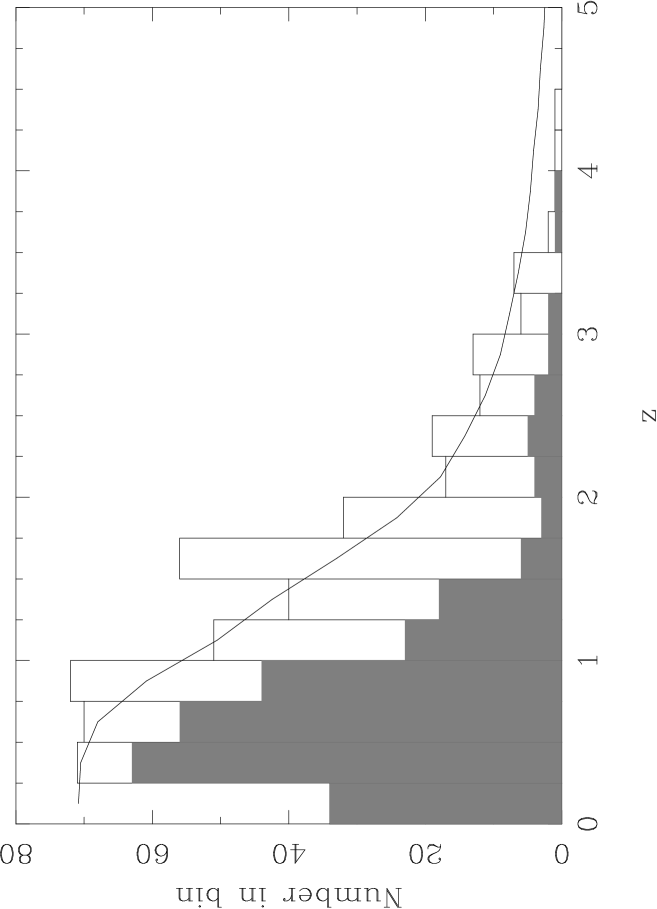
Figure 4: Histogram of redshifts for the 100-$\mu$Jy sample. The shaded region of the histogram indicates spectroscopic redshifts only, while the open bars represent the photometric redshifts. The solid line shows the predicted distribution from the SKA Simulated Skies (Wilman et al. 2008), renormalized to have the same total number of sources.

The photometric redshifts were derived using the code eazy (Brammer, van Dokkum, & Coppi 2008) after correcting the observed photometry for the Galactic extinction of $A_{V}=0.070$ (Schlegel, Finkbeiner & Davis 1998) with the Milky Way extinction law of Pei (1992). All but seven objects have images in eleven filters (u^∗BVRi^′z^′JHK plus IRAC channels 1 and 2), while those seven possess u^∗RIJHK and IRAC images. However, not all these images provide useful photometry for all targets due to nearby bright sources, and these instances are noted in Table 1.

As noted by Simpson & Eisenhardt (1999), IRAC photometry can be important for constraining photometric redshifts through the H^- opacity minimum, which appears as a bump in the spectra of galaxies at a rest-frame wavelength of 1.6 $\mu$m. However, this feature can be absent in AGNs due to thermal emission from hot dust in the obscuring torus, resulting in a spectral energy distribution that continues to rise at longer wavelengths and hence an incorrectly high photometric redshift. After some experimentation it was found that the number of catastrophic outliers in the $z_{\rm spec}$–$z_{\rm phot}$ plane could be reduced by adding an additional 10 per cent uncertainty in quadrature to the IRAC fluxes. In assigning a photometric redshift to each object we use the probability-weighted mean redshift, rather than the most probable redshift. This ensures that the photometric redshift always lies within the central 68 per cent confidence interval, which we also list in Table 1 The luminosity–redshift plane for our sample in shown in Fig. 1.

Fig. 2 compares the photometric and spectroscopic redshifts for the 267 sources with spectroscopic redshifts. Very good agreement is seen over the range $0<z<1.4$, beyond which the spectroscopic completeness falls rapidly. The number of catastrophic outliers also increases at $z_{\rm phot}>1$, but this can be attributed to a strong bias in the types of sources with spectroscopic redshifts $z_{\rm spec}>1$. It is difficult to obtain absorption-line redshifts for distant objects due to the fainter continuum and hence reduced signal-to-noise ratio, and the redshifting of strong features (such as the Ca HK doublet) to wavelengths affected by night sky emission lines and/or detector fringing. As a result, many of the sources with spectroscopic redshifts $z>1$ are AGNs whose broad-band photometry is affected by strong emission lines and dust emission. Nevertheless, as Fig. 3 shows, the scatter in the $z_{\rm phot}$–$z_{\rm spec}$ relation is very small, and only 5 per cent (11/242) of the sources not classified as ‘BLAGN’ are catastrophic outliers. Since optically-bright sources and those with X-ray emission have been preferentially targeted by the spectroscopic observations described in Section 2.2 we expect there to be few, if any, broad-line AGNs lacking a spectroscopic redshift.

We compare our redshift distribution with that from the SKA Simulated Skies (S³; Wilman et al. 2008), which provides a mock catalogue of extragalactic radio sources over a $20\times 20$ deg² area of sky. The S³ simulations predict 699 sources with $S_{\rm 1.4GHz}>100\,\mu$Jy over our 0.808-deg² survey area, but we detected 505 and expect 539 after accounting for incompleteness near the flux limit (see table 2 of Paper I). We already noted in Paper I that the source counts in the SXDF appear to be significantly lower than those in some other fields, and we have simply renormalized the total number of sources in the simulations by 539/699. There is good agreement between the renormalized model and observations, except in the lowest redshift bin ($z<0.25$). We speculate that this is due to radio sources which were resolved in our observations and hence failed to satisfy the criterion $S_{\rm peak}>100\,\mu$Jy despite having a total flux density in excess of the threshold. The deficit in this bin is consistent with the estimated number of sources missed by our selection on peak flux density (34).

4 Discussion

4.1 The stellar populations of radio sources

Figure 5: A simple characterisation of the best-fitting stellar populations found by eazy for objects with spectroscopic redshifts and classifications. The abscissa shows the fraction of the rest-frame $V$-band light produced by the three old stellar populations, and the ordinate shows the fraction of the rest-frame $K$-band light produced by the young dust-reddened population. Large filled symbols represent objects without emission lines (‘Abs’ in Table 1), and open symbols are objects with weak line emission (‘Weak’ in Table 1). Small points are sources with other classifications. Objects discussed in the text are labelled with their source numbers.

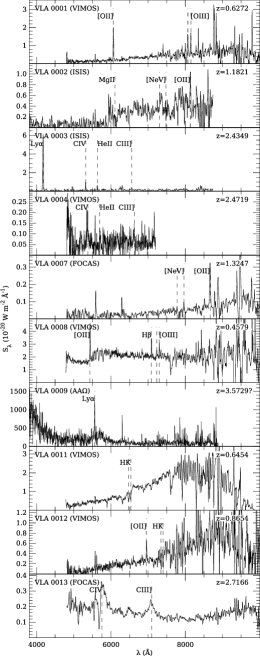
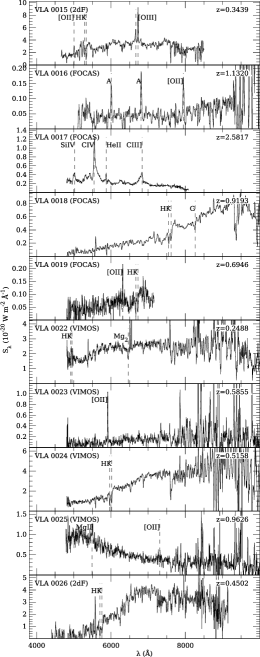
Figure 14: Spectroscopy of SXDF radio sources. The names of the sources and the origin of the spectra are shown in the top left corner of each panel, while the redshift is displayed in the top right. Identified features are marked with vertical dashed lines and labelled. An ‘A’ indicates a feature is an artifact. Some spectra have been lightly smoothed or had strong artifacts interpolated across for presentation purposes.

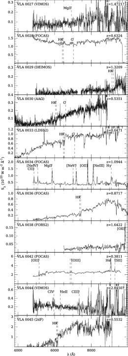
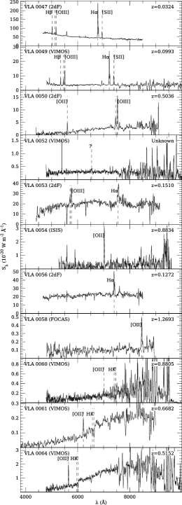
Figure 14: continued.

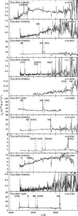
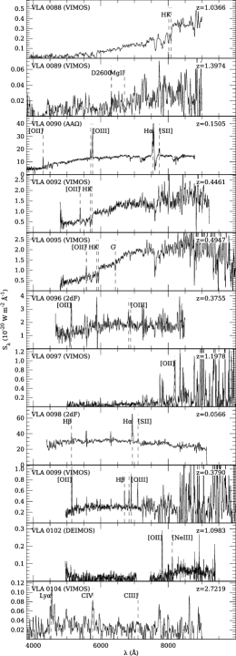
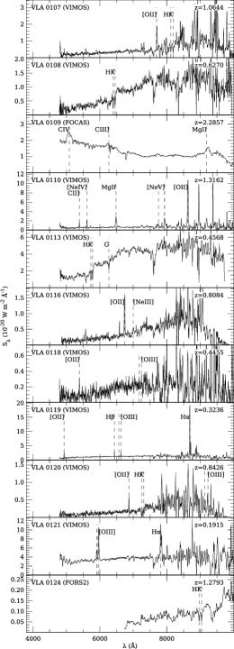
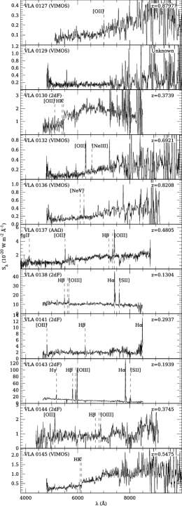
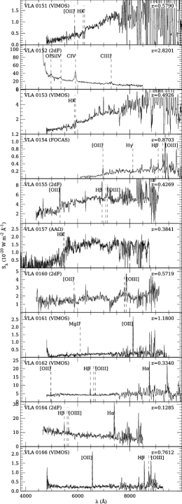
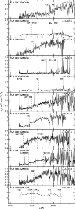
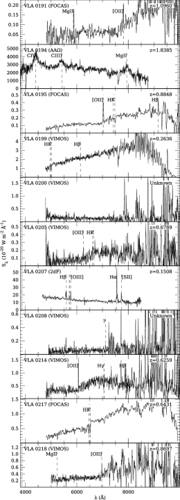
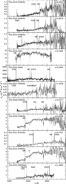
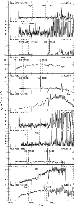
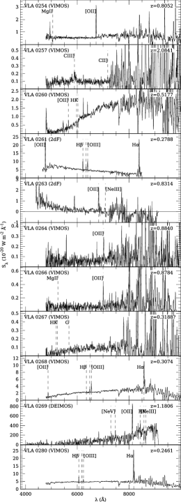
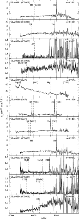
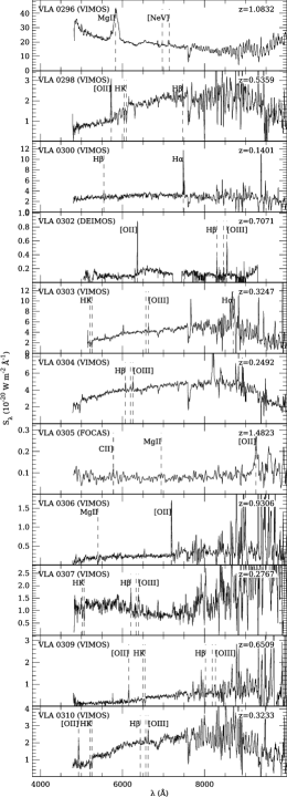
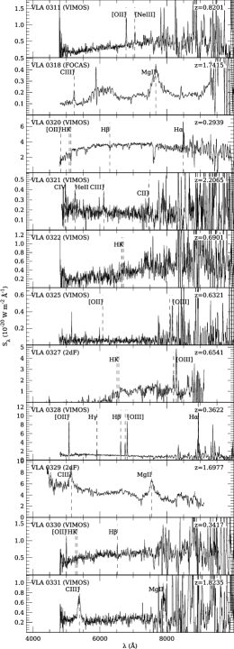
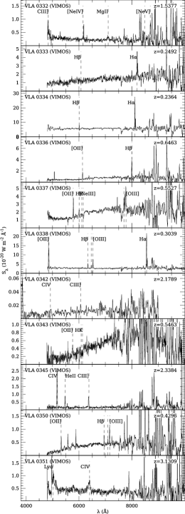
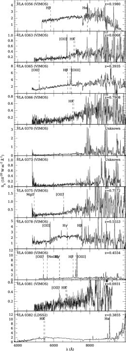
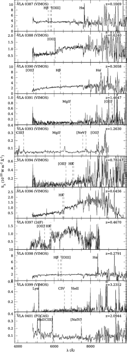
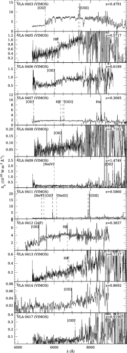
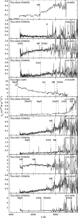
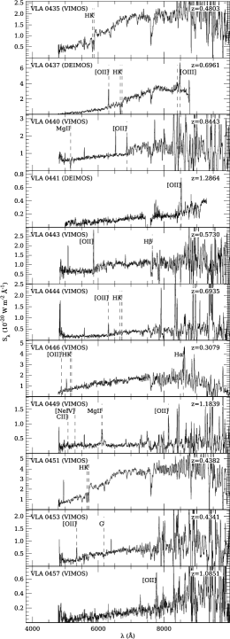
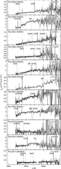
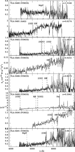
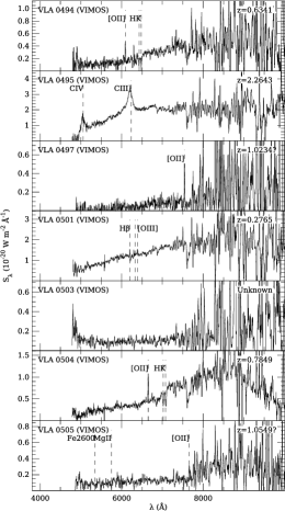
Figure 14: continued.

eazy derives its photometric redshifts by fitting a linear combination of six synthetic stellar population spectra to the observed broadband fluxes. These spectra have non-trivial star formation histories but three can be considered ‘old’ and three ‘young’, including one dusty starburst spectrum. We choose to characterise the stellar population of the best-fitting model with two numbers: the fraction of rest-frame $V$-band light which arises from old stars (i.e., the fraction from the three ‘old’ templates), $f_{{\rm old},V}$, and the fraction of rest-frame $K$-band light produced by the dusty starburst template, $f_{{\rm dusty},K}$. When we compare this to the spectroscopic classifications (Fig. 5), there is a clear correspondence between objects classified as ‘old’ and those lacking emission lines. Outliers are labelled in the figure, and their locations are readily understood. The photometric measurements of VLA 0033 and VLA 0382 are contaminated by nearby objects (a $z>1$ gravitationally-lensed arc in the case of VLA 0033; see Geach et al. 2007 for more details). VLA 0028 is unusual in that, while clearly resolved at longer wavelengths, it appears stellar in the $u^{*}$ and $B$ filters. This can also be seen in the unusual ‘concave’ nature of its spectrum in Fig. 14. It may be a chance superposition of an early-type Galactic star with the radio galaxy, or the galaxy may harbour a BL Lac nucleus.

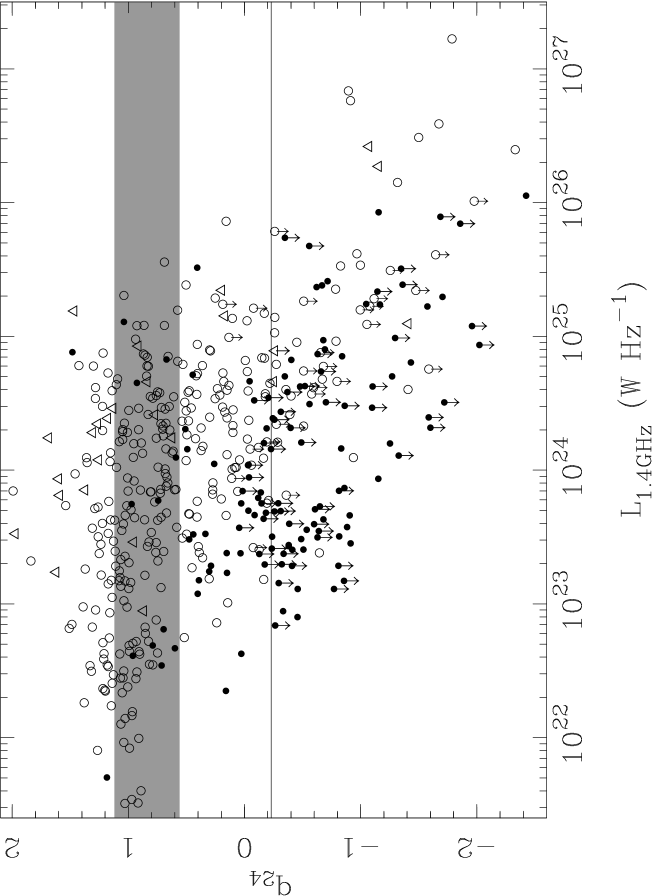
Figure 6: Plot of $k$-corrected $q_{24}$ values against 1.4-GHz luminosity density. Objects classified as BLAGN are shows as triangles. Filled symbols indicate galaxies whose stellar populations are classified as ‘old’ according to the criterion of Section 4.1. The shaded region shows the $\pm 1\sigma$ range for star-forming galaxies from Appleton et al. (2004), while the horizontal line indicates Ibar et al.’s (2008) boundary between radio-loud and radio-quiet sources, which we also adopt.

The criterion $f_{{\rm old},V}>0.82$ selects 90% (52/58) of sources classified as ‘Weak’ or ‘Abs’, but only 11% (21/192) of other sources, and we therefore use this criterion to identify host galaxies without any significant recent star-formation activity or strong unobscured accretion, which we term ‘old’. We independently assess this criterion by using 24-$\mu$m imaging from the SpUDS Spitzer survey (PI: J. Dunlop) to identify objects with strong star-formation or accretion activity. Due to the high source density of this image, we follow the method of Rodighiero et al. (2006) by running the clean algorithm (Högbom 1974) on the image to reduce the effects of confusion from the Airy rings. The cleaned image is then convolved with a Gaussian of FWHM 5.5^′′ and added to the residual image. A 24-$\mu$m flux density is measured for each radio source by fitting a Gaussian at its location in this image. Where this fit was affected by a nearby 24-$\mu$m source we employed a ‘search and destroy’ method to eliminate such sources before fitting a point spread function to the counterpart. We $k$-correct the 24-$\mu$m photometry using Silva et al.’s (1998) model fit to the spectral energy distribution of M82, which we convolve with the transmission profile of the MIPS filter. We have also undertaken all subsequent analysis assuming an AGN-like spectral energy distribution that is flat in $\nu L_{\nu}$ and find no significant differences in our results. After $k$-correcting the 1.4-GHz radio flux, we compute the ratio of mid-infrared to radio flux $q_{24}=\log(S_{\rm 24\mu m}/S_{\rm 1.4GHz})$. This quantity identifies radio-loud AGNs which lie away from the tight infrared–radio correlation that is obeyed by both star-forming galaxies and radio-quiet AGNs (e.g., Sopp & Alexander 1991).

In Fig. 6 we plot $q_{24}$ against radio luminosity and indicate which galaxies have been classified as ‘old’ by our criterion. We also plot a line at $q_{24}=-0.23$, which Ibar et al. (2008) used to select radio-loud galaxies: this is equivalent to a radio-loudness parameter $R\approx 30$ (cf. Kellermann et al. 1989) if we assume the relationship between 24-$\mu$m and $B$-band luminosities implied by the radio-loud QSO spectral energy distribution of Shang et al. (2011). It is clear that old galaxies do not represent a random sample of the population, with the fraction of old galaxies among the radio-loud population decreases from nearly 100 per cent at $L_{\rm 1.4GHz}\sim 10^{23}\rm\,W\,Hz^{-1}$ to almost zero at $L_{\rm 1.4GHz}>10^{26}\rm\,W\,Hz^{-1}$. This can be understood as a result of the Hine & Longair Class A fraction increasing with luminosity, since these objects possess a strong non-stellar ionizing continuum (which may be obscured) and also frequently show evidence for recent star formation (see Tadhunter et al. 2011 and references therein), both of which would prevent the host galaxy from being classified as old. Class B sources dominate at lower radio luminosities and these sources usually display the spectra of old stellar populations.

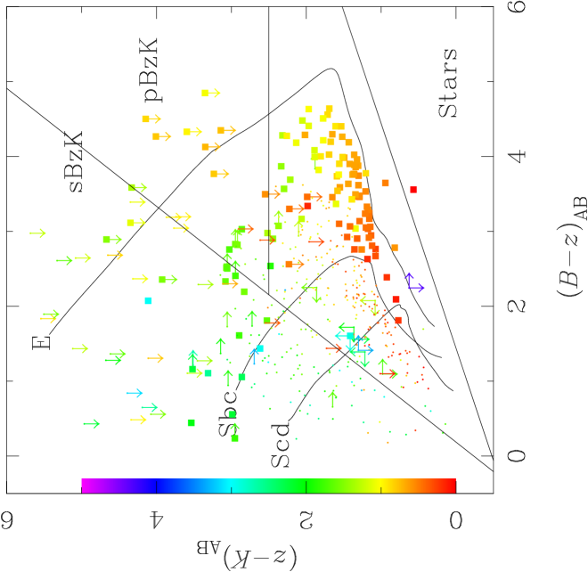
Figure 7: Colour–colour plot for all radio sources, colour-coded according to their redshifts (spectroscopic where available, otherwise photometric), as indicated by the bar on the $y$-axis. Large filled symbols indicate objects classified as ‘old’ according to the criterion in the text. The parameter space is split in the manner of Daddi et al. (2004), after applying photometric corrections to account for filter differences (W. Hartley, private communication). The loci of non-evolving galaxy templates from Coleman, Wu, & Weedman (1980) are plotted (W. Hartley, private communication).

We compare our classification with the locations of sources in the BzK colour–colour diagram of Daddi et al. (2004) in Fig. 7, where we also plot the loci of the non-evolving E, Sbc, and Scd galaxy templates from Coleman, Wu, & Weedman (1980). This diagram is used to select galaxies at $z\ga 1.4$ and classify them as either passively-evolving (pBzK) or star-forming (sBzK) objects. Surprisingly, the pBzK region of this diagram contains very few sources, with the locus of ‘passive’ radio galaxies lying between the E and Sbc curves. Since passive galaxies at $z>1.4$ have very red $(B-z)$ colours, even a small amount of ultraviolet luminosity will cause galaxies to migrate from the pBzK region into the sBzK region of the diagram, as is apparent from the presence of ‘old’ galaxies in the sBzK region of the diagram. It therefore appears that there is some ultraviolet emission associated with AGN activity even in sources which display no line emission but we cannot say whether this arises from stellar or non-stellar processes. We conclude from Figures 6 and 7 that our criterion for selecting old galaxies is reliable although it is not as severe as the pBzK criterion.

4.2 The K–z relation for faint radio sources

It is well-known that radio galaxies (i.e., the host galaxies of radio-loud AGNs) follow a tight locus in the $K$-band Hubble diagram, the so-called $K$–$z$ relation (Lilly & Longair 1984; Jarvis et al. 2001; De Breuck et al. 2002; Willott et al. 2003). Historically, the $K$-band magnitudes used in this diagram have been measured in a fixed metric aperture of 63.9 kpc diameter, which corresponds to $\sim 8^{\prime\prime}$ at high redshift. However, the compact nature of distant radio galaxies means that the magnitudes are almost universally measured in smaller apertures to reduce the photometric uncertainty, and then an offset is applied based on an assumed curve of growth (the prescription of Eales et al. 1997 is frequently followed). While this does, in principle, enable objects from different samples to be plotted on the same plot, it is only valid if all objects obey the same curve of growth, or have all had their photometry measured in identical angular apertures so that the same offset is applied to all. The Eales et al. (1997) prescription was derived for bright radio sources which are known to be massive ellipticals, but this is clearly not applicable to sources from fainter radio samples such as the one studied here. We therefore follow Bryant et al. (2009a) in using apertures of the same angular size (4-arcsecond diameter) at all redshifts. Once again, we apply a correction to the 2MASS photometry and, following the method in Section 3.1.1, we determine $K_{\rm 2MASS}(\phi 4^{\prime\prime})-K_{\rm UDS}(\phi 4^{\prime\prime})=0.35$. These measurements are also quoted in Table 1.

Figure 8: Plot of $K$-band magnitude ($\phi 4^{\prime\prime}$) against 1.4-GHz radio flux density. Large symbols show the median $K$ magnitude in each flux density bin, derived from the unbiased subset of objects with UDS photometry. The vertical error bars show the 16th and 84th percentiles of the distribution in each bin, while the boxes show the 1$\sigma$ uncertainty on the median estimated from 500 bootstrapped samples.

In Paper I we showed that there was no significant change in the optical colours of radio sources over the radio flux density range $0.1{\rm\,mJy}\leq S_{\rm 1.4GHz}<100\rm\,mJy$, and inferred that, although present, a population of star-forming galaxies could not be dominating at the faintest fluxes. Fig. 8 shows that there is also no significant variation in the median $K$-band magnitudes of radio sources as a function of radio flux density.

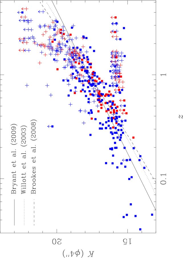
Figure 9: $K$-band Hubble diagram for the SXDF 100-$\mu$Jy sample. Squares indicate spectroscopic redshifts, while crosses show objects with photometric redshift estimates only. Red and blue points indicate radio-loud and radio-quiet sources, respectively. The lines indicate the $K$–$z$ relations from Bryant et al. (2009b; fit over the entire redshift range), Willott et al. (2003), and Brookes et al. (2008). The relations from the latter two papers have been corrected to our 4-arcsec aperture using the prescription of Eales et al. (1997).

The original $K$–$z$ relation was determined for the most powerful radio sources from the 3C catalogue (Lilly & Longair 1984) and, as deeper radio surveys have been undertaken, a number of papers have appeared in the literature investigating the variation in the $K$–$z$ relation with radio luminosity. Eales et al. (1997) and Willott et al. (2003) showed that galaxies from the fainter 6C and 7C catalogues were 0.6 magnitudes fainter at a given redshift which, after excluding a direct correlation with AGN luminosity (Leyshon & Eales 1998; Simpson, Rawlings & Lacy 1999), was determined to be due to a difference in the stellar luminosities of their host galaxies. However, the faintest of these samples (7C) has a radio flux limit approximately 1000 times brighter than that of our sample, compared to a factor of only 20 between 7C and 3C. Vardoulaki et al. (2012) extended this analysis a further factor of $\sim 30$ using the bright SXDF sample of Paper II and identified sources significantly fainter than the $K$–$z$ relation. A problem with the analysis of faint samples is that the strong correlation between emission-line and radio luminosity (e.g., Rawlings & Saunders 1991) means that sources from fainter samples will have lower line fluxes, frequently resulting in the (often marginal) detection of only a single line. While in some cases this line can be confidently identified due to the absence of other lines, many authors have used the observed $K$ magnitude to support an identification (we stress that Vardoulaki et al. do not do this). This leads to circular reasoning because objects are placed on the $K$–$z$ at least partly under the assumption that the $K$–$z$ relation is reliable, and these objects are then used to support that very assumption. We reiterate that all the spectroscopic redshifts presented here are based solely on the results of the spectroscopy, and in Fig. 9 we plot the $K$-band Hubble diagram for our sample. We include on this plot the $K$–$z$ relation of Bryant et al. (2009), plus those presented by Willott et al. (2003) and Brookes et al. (2008), both of which have been corrected to our fixed angular-diameter aperture using the same method from Eales et al. (1997) that they used to correct their data to the standard 63.9-kpc aperture. The relation of Brookes et al. differs from the other two in that the least-squares fit minimized the residuals in $z$, rather than $K$, since $K$ is the independent variable when the relation is used to infer redshifts. It is also derived from a radio source sample that is fainter than those of Willott et al. and Bryant et al., although the radio flux limit is still 72 times brighter than ours. Fig. 9 shows quite clearly that all three $K$–$z$ relations fail to provide a good fit to our data at $z\ga 1$, where the sources are systematically fainter than the relation.

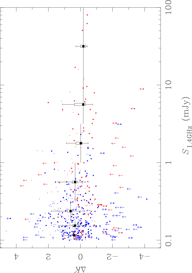
Figure 10: Plot of the deviation from the $K$–$z$ relation of Bryant et al. (2009b) against 1.4-GHz radio flux density. Filled squares show objects with spectroscopic redshifts. The large filled circles show the median $K$ magnitude in each flux density bin, derived from the unbiased subset of objects with UDS photometry. The vertical error bars and boxes have the same meaning as in Fig. 8.

Table 2: Median $K$ magnitude offset from the $K$–$z$ relations of Fig. 9 for our $z>1$ sources. The error bars indicate the 1$\sigma$ uncertainty in the median from 500 bootstrapped samples.

$S_{\rm 1.4GHz}$		Median offset from $K$–$z$ relation
(mJy)		Bryant	Willott	Brookes
10.000–	100.000	$-0.13^{+0.25}_{-0.10}$	$-0.23^{+0.29}_{-0.07}$	$-0.42^{+0.26}_{-0.08}$
3.162–	10.000	$0.64^{+0.47}_{-0.19}$	$0.61^{+0.33}_{-0.23}$	$0.41^{+0.20}_{-0.25}$
1.000–	3.162	$0.28^{+0.19}_{-0.31}$	$0.35^{+0.02}_{-0.29}$	$0.08^{+0.08}_{-0.06}$
0.316–	1.000	$0.52^{+0.16}_{-0.17}$	$0.40^{+0.22}_{-0.11}$	$0.18^{+0.17}_{-0.12}$
0.178–	0.316	$0.96^{+0.24}_{-0.11}$	$0.92^{+0.21}_{-0.13}$	$0.73^{+0.16}_{-0.16}$
0.133–	0.178	$0.69^{+0.23}_{-0.22}$	$0.69^{+0.13}_{-0.24}$	$0.44^{+0.16}_{-0.27}$
0.100–	0.133	$0.57^{+0.05}_{-0.12}$	$0.52^{+0.06}_{-0.14}$	$0.25^{+0.08}_{-0.10}$

We also show the classification of sources as radio-loud or radio-quiet in this figure, based on the analysis of Section 4.1. For sources outside the SpUDS region or with $q_{24}$ upper limits larger than $-$0.23, where we cannot make a conclusive determination as to whether they are radio-loud or radio-quiet, we use the result of Fig. 6 to identify ‘old’ galaxies as being radio-loud. Although the redshift distributions of the radio-loud and radio-quiet populations differ, with the lowest-redshift sources being exclusively radio-quiet, it is clear that this deviation from the $K$–$z$ relation is not simply caused by the presence of radio-quiet sources in the sample.

We investigate further by plotting the deviation from the $K$–$z$ relation of Bryant et al. (2009b) against radio flux density in Fig. 10. Using only the unbiased set of objects within the UDS region and including magnitude limits, the Kendall’s rank correlation statistic (Brown, Hollander & Korwar 1974; Isobe, Feigelson & Nelson 1986) indicates the presence of an anticorrelation between these quantities at greater than 95 per cent significance. If only those objects with secure spectroscopic redshifts are used, the level of significance is slightly lower (92 per cent), but this subsample suffers from numerous biases that are hard to quantify, such as a bias against objects with low emission-line fluxes, or those in the ‘redshift desert’.

This result is not caused by our choice of $K$–$z$ relation. Table 2 shows the median offset of our $z>1$ sources from each of the three relations. We consider only the highest-redshift sources since these are the ones for which this form of redshift estimator is most likely to be used, and the differences between the different relations is dominated by aperture corrections at low redshift. We also undertake this analysis for radio-loud and radio-quiet sources separately, and find no significant difference between the two samples. We find that the sub-mJy radio sources are systematically fainter than the $K$–$z$ relations by up to a magnitude, resulting in the overestimation of redshifts and hence luminosities (by up to a factor of two). In reality, however, the use of a combination of spectroscopic redshifts and those estimated from the $K$–$z$ relation will produce larger errors. As Fig. 10 clearly shows, the distribution of deviations is not symmetric about the median but has a tail to even fainter magnitudes, and it is these objects which are less likely to have measured spectroscopic redshifts. Results that stem from the use of ‘single-band photometric redshifts’, or from spectroscopic redshifts derived from a single emission line plus a broad-band magnitude, must therefore be treated with extreme caution. This bias can only be eliminated by estimating the redshift of a source based on its $K$ magnitude and radio flux density, and also whether or not spectroscopy has been attempted, using an extension of the method of Cruz et al. (2007). However, this requires a faint radio sample with 100 per cent reliable redshifts and that does not yet exist.

4.3 Evolution of the radio luminosity function

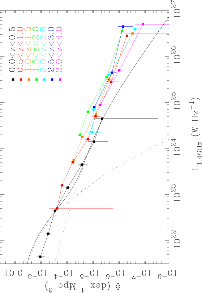
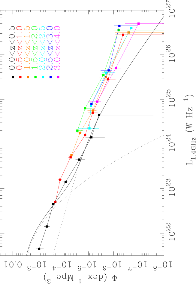
Figure 11: Evolution of the radio luminosity function with redshift for the SXDF sample. The left-hand plot ignores photometric redshift uncertainties, while the right-hand plot incorporates these using 1000 Monte Carlo realizations as described in the text, with the error bars indicating the range between the 16th and 84th percentile for each data point. Different colour symbols denote different redshift ranges as indicated in the key. Bins are of of width $\Delta\log L_{\rm 1.4GHz}=0.5$ for $L_{\rm 1.4GHz}\leq 10^{25}$ W Hz^-1 and $\Delta\log L_{\rm 1.4GHz}=1.0$ at higher luminosities. Points have only been plotted where there is at least one object in the bin, and points within the same luminosity bin representing different redshift bins are offset horizontally for clarity. The black solid line is the parametrized fit to the local radio luminosity function of Mauch & Sadler (2007), and the dotted curves show the separate contributions from star-forming galaxies and AGNs.

At the flux densities we are studying, the extragalactic radio source counts are comprised of (at least) four populations: star-forming galaxies, radio-quiet AGNs, and two types of radio-loud AGN. Due to their physically distinct natures, these populations need not undergo similar evolution and therefore an accurate parametrization of the RLF and its evolution is not a realistic proposition. Instead we construct binned luminosity functions using the method of Page & Carrera (2000) and present these in Fig. 11. The error bars in Fig. 11(a) account for only the Poisson errors and ignore the photometric redshift uncertainties, while we have propagated these uncertainties to produce Fig. 11(b) by running 1000 Monte Carlo realisations where each source without a spectroscopic redshift is assigned a photometric redshift based on the probability density function returned by eazy. We calculate the asymmetric 1-$\sigma$ error bar from the 16th and 84th percentiles of the distribution in each bin and add this in quadrature to the Poisson uncertainty. Unsurprisingly, the contribution to the error budget from the photometric redshift uncertainty increases with redshift as the hosts become fainter and the photometric errors grow. There will also be a further contribution to the error budget from our lack of knowledge of the sources’ spectral indices and a systematic effect caused by spectral curvature (e.g., Jarvis & Rawlings 2000), although we presently lack sufficiently deep multifrequency radio data to quantify these effects. Accounting for the photometric redshift uncertainties is important since we can construct the RLF for all radio sources (except the seven sources described in Section 3.2 whose photometry is contaminated by nearby objects), even if they lack a formal optical or infrared counterpart. We have not corrected for incompleteness towards marginally-resolved sources near the radio flux limit since Fig. 4 suggests that this only affects objects in the lowest redshift bin. Indeed, the difference between our $z<0.5$ RLF and that of Mauch & Sadler (2007) in Fig. 11 supports this suggestion.

The radio source population shows strong evolution out to $z\sim 1$ over the entire luminosity range probed by our sample, with the space density of these objects increasing by a factor of 3 over this lookback time. The evolution is stronger for higher luminosity radio sources when our results are compared with the local RLF. This is consistent with the evolution found by Sadler et al. (2007) in their comparison between the 6dFGS and 2SLAQ radio galaxy samples. At higher redshift, there appears to be a slowing down of this evolution and there is a hint of negative evolution at higher redshift, with the space densities at $z>2$ being systematically lower than at later cosmic times, albeit at very low significance. This is not straightforward to interpret due the composition of the radio population evolving at these intermediate luminosities. Locally, sources with $L_{\rm 1.4GHz}\sim 10^{24{\rm-}26}\rm\,W\,Hz^{-1}$ belong to Hine & Longair’s Class B and are massive ellipticals engaged in a constant cycle of heating infalling gas so as to prevent additional star formation, operating in what Croton et al. (2006) dub ‘radio-mode’ feedback. However, as lookback time increases, the strong evolution in the number of rapidly star-forming galaxies and luminous radio-quiet AGNs causes these to become significant contributors. For example, $L_{\rm 1.4GHz}=10^{24}\rm\,W\,Hz^{-1}$ corresponds to a star-formation rate of $\sim 200\rm\,M_{\odot}\,yr^{-1}$ in $M>5\rm\,M_{\odot}$ stars (Condon 1992), or $\sim 540\rm\,M_{\odot}\,yr^{-1}$ in all stars above 0.08 M_⊙ using the Kroupa (2001) initial mass function and, while such objects are rare in the local Universe, they are found in submillimetre surveys with a redshift distribution that peaks at $z\sim 2$ (e.g., Chapman et al. 2005).

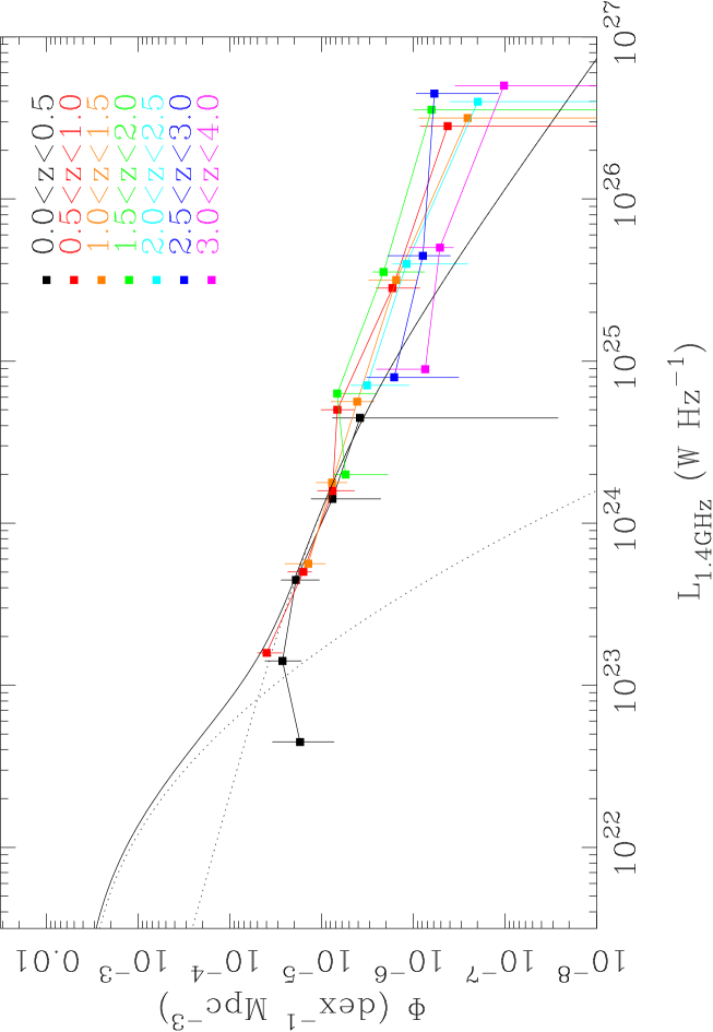
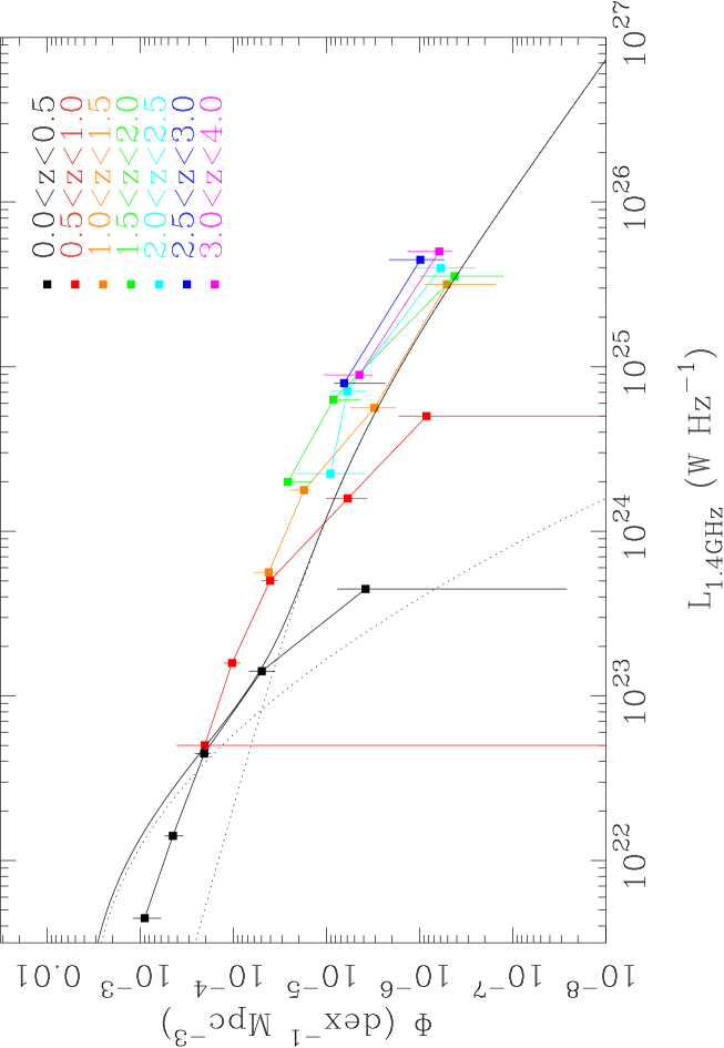
Figure 12: Evolution of the radio luminosity function for (a) radio-loud and (b) radio-quiet galaxies. We define galaxies as radio-loud if they have $q_{24}<-0.23$ or have $q_{24}$ upper limits greater than this value and have been classified as ‘old’ in Fig. 5.

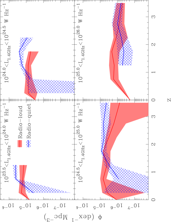
Figure 13: Plots of the redshift evolution of the space density of radio sources from Fig. 12, binned by luminosity. The shaded regions show the 1-$\sigma$ uncertainties in each bin. The radio-loud curves have been extended to $z=0$ using the Mauch & Sadler (2007) AGN radio luminosity function, since this is dominated locally by radio-loud objects at these luminosities.

We next investigate the evolution of the radio-loud and radio-quiet subpopulations independently, again running 1000 Monte Carlo trials to quantify the effect on the RLF of the photometric redshift uncertainties and reclassifying objects as radio-loud or radio-quiet based on their new $k$-corrected $q_{24}$ values. This results in the luminosity functions shown in Fig. 12. We see first that this split agrees fairly well at low redshift with the separate AGN and star-formation RLFs of Mauch & Sadler (2007), despite the fact that radio-quiet AGNs are grouped with star-forming galaxies in our classification scheme but with radio-loud AGNs by Mauch & Sadler. Such objects comprise only a few per cent of the 6dFGS–NVSS sample and so the RLF is not particularly sensitive to their classification except at the bright end of the radio-quiet RLF, where AGNs dominate over star-forming galaxies (we note also the recent claim that the radio emission from some radio-quiet AGNs may be powered by star formation; Kimball et al. 2011). It is also clear that the evolution at intermediate radio luminosities is driven by the radio-quiet sources, as we find zero or negative evolution among the radio-loud sources with $L_{\rm 1.4GHz}\la 10^{24}\rm\,W\,Hz^{-1}$. This agrees with the finding of Padovani et al. (2011) and Fig. 13 shows very clearly that the space density of radio-quiet sources can exceed that of radio-loud ones, even at radio luminosities close to the Fanaroff–Riley break. At $L_{\rm 1.4GHz}\approx 10^{24}\rm\,W\,Hz^{-1}$ the radio-quiet sources outnumber the radio-loud ones by $z\sim 1$ as one looks to earlier cosmic epochs, whereas this does not happen until $z\sim 2$ for sources with $L_{\rm 1.4GHz}\approx 10^{25}\rm\,W\,Hz^{-1}$.

Fig. 13 also shows hints of a decline in the space density of radio-loud galaxies at $z\ga 1$, and this decline appears to happen later (i.e., at lower redshift) for lower-luminosity objects. Similar claims have been made by Waddington et al. (2001) and Rigby et al. (2011) and our results are quantitatively consistent with these claims, although we fail to robustly identify the turnover at $z\sim 1$ for sources with $L_{\rm 1.4GHz}>10^{25}\rm\,W\,Hz^{-1}$ claimed by Rigby et al. Any decline of the radio-quiet population is less severe and/or happens at higher redshift where we lack sensitivity. Although we do not separate our radio-quiet sources into AGN and star-forming subsamples, we note that Padovani et al. (2011) found very similar evolution for these two samples in their study of radio sources in the Chandra Deep Field South, and we find similarly strong evolution. At luminosities where star-forming galaxies dominate locally ($L_{\rm 1.4GHz}\sim 10^{23}\rm\,W\,Hz^{-1}$) we see evolution of the space density that is consistent with the increase in the cosmic star formation density (e.g., fig. 1 of Hopkins & Beacom 2006). At higher luminosities, where the population is composed of radio-quiet AGNs, the evolution over the range $0.5\la z\la 2$ is consistent with the rapid increase in the number of optically-selected QSOs (e.g., Croom et al. 2004). Adopting the radio-quiet QSO spectral energy distribution of Shang et al. (2011), radio-quiet QSOs with $L_{1.4GHz}=10^{25}\rm\,W\,Hz^{-1}$ should have $M_{b_{J}}\approx-27$ but the space density of the former is several times greater than that of the latter. This is readily explained by a combination of two factors. First, the radio-selected sample includes not just optically-bright QSOs but also obscured AGNs. These can be ‘Type 2’ objects of the unified model (e.g., VLA0074) or ‘host-obscured’ objects that Martínez-Sansigre et al. (2008) claim dominate the accretion onto supermassive black holes. Second, radio selection will inevitably find the ‘radio-intermediate’ objects that are believed to be Doppler-boosted radio-quiet sources (Falcke, Sherwood & Patnaik 1996) and therefore have fainter optical luminosities.

The luminosity-dependent turnover in the space density of radio-loud AGNs appears to be similar to the finding of Fiore et al. (2003) that the space density of luminous X-ray-selected AGNs peaks at a higher redshift than the space density of lower-luminosity sources. Both results have been explained in the context of ‘downsizing’ but radio selection produces a more complex sample than shorter-wavelength selection methods. This is because other selection methods (e.g., optical or X-ray) can only find supermassive black holes that are undergoing radiatively-efficient accretion (‘quasar mode’) and there is a correlation between luminosity and black hole mass because the range of black hole masses is greater than the spread in Eddington ratios (e.g., Kelly et al. 2010). However, radio selection also finds black holes that are accreting in a radiatively-inefficient mode (‘radio mode’) so this correlation is broken as one moves below the Hine & Longair boundary.

To understand this result we first turn to the work of Best et al. (2005a,b) who determined the fraction, $f_{\rm radio-loud}$, of galaxies in the local Universe brighter than some 1.4-GHz luminosity, $L$, as a function of black hole mass, estimated from the stellar velocity dispersion. They found that more massive black holes (in more massive galaxies) were more likely to host the most luminous radio sources and derived an expression for $f_{\rm radio-loud}$ as a function of $L$ and black hole mass, $M$. From this definition, it follows that the probability that a galaxy with a given black hole mass has a radio luminosity between $L$ and $L+dL$ is given by

$$p(L|M)\,dL=-\frac{\partial f_{\rm radio-loud}}{\partial L}\,dL$$ (2)

and hence the overall RLF is given by

$$\Phi(L)=\int\phi(M)\,p(L|M)\,dM\,,$$ (3)

where $\phi(M)$ is the black hole mass function. However, Best et al. (2005b) were able to write the functional form of $f_{\rm radio-loud}$ in a manner that is separable in $L$ and $M$ and, for any such separable form,

$$f_{\rm radio-loud}=f(L)\,g(M)$$ (4)

we can write

$$\Phi(L)=-f^{\prime}(L)\int\phi(M)\,g(M)\,dM\,,$$ (5)

where $f^{\prime}(L)$ is the first derivative of $f(L)$ with respect to luminosity. The shape of the RLF is therefore independent of the black hole mass distribution if Best et al.’s expression for $f_{\rm radio-loud}$ is true at all redshifts. However, their sample was dominated by Hine & Longair Class B objects and the expression might not be applicable to Class A objects due to the different mode of accretion. Nonetheless, in a general sense, if the likelihood of a black hole powering a radio-loud AGN increases with its mass and $\phi(M)$ has a Schechter-like form with a sharp cutoff at high mass (e.g., Graham et al. 2007), it is black holes with masses near the characteristic mass, $M^{*}$, that drive the overall shape of the RLF.

In the most recent theoretical models for the evolution of supermassive black holes, radio jets are powered by the Blandford–Znajek mechanism (Blandford & Znajek 1977) and the radio jet power is a function of the black hole spin (e.g., Fanidakis et al. 2011; Martínez-Sansigre & Rawlings 2011). The panels in Fig. 13 therefore represent different black hole spins, with the lowest luminosity objects having the lowest spins. The luminosity-dependent turnover is therefore due to slowly-rotating black holes becoming radio-loud AGNs at a later cosmic epoch and one can speculate on plausible scenarios for this. For example, a major galaxy merger can produce a rapidly-spinning black hole (e.g., Wilson & Colbert 1995) as well as promoting vigorous star formation that exhausts the cold gas supply, leading to a luminous radio mode AGN. Galaxies that do not undergo such mergers will not have their black holes spun up and will retain their cold gas for longer, allowing them to operate in quasar-mode until a later cosmic epoch when they eventually become low-luminosity radio mode AGNs.

A major observational challenge that hampers further study of the radio-mode AGN population’s evolution is the difficulty in separating these objects from the rapidly evolving quasar-mode sources, both radio-loud and radio-quiet. If this is to be done by using the infrared–radio correlation, as we have, it requires mid-infrared imaging to levels $\ll 1\,$mJy, which is beyond the capabilities of Herschel and hence is only possible in the immediate future within the regions of sky that already possess deep MIPS imaging. These cover just a few square degrees of the sky and so this method is not suitable for the analysis of faint radio sources from the large-area surveys about to be undertaken by new radio telescopes. Section 4.1 suggests that a method based on the stellar population of the host galaxy might be viable, and this is supported by the work of Best & Heckman (2011).

5 Summary

We have presented spectra for 277 of the 505 radio sources in the sample of Simpson et al. (2006), with reliable redshifts for 256, and a further 11 possible redshifts. Spectroscopic observations of a further 129 sources failed to produce any significant continuum or line detections. Photometric redshifts have been derived for the entire sample, bar seven sources strongly affected by foreground objects.

We have found the observed redshift distribution of our sources to be consistent with that predicted by recent semi-empirical simulations, and have found that the median $K$-band magnitude of radio sources does not change with radio flux density. However, we have demonstrated that sources with $S_{\rm 1.4GHz}\la 1$ mJy are systematically offset from the $K$–$z$ relation to fainter magnitudes, compared to sources at brighter radio fluxes. This argues strongly against the use of ‘single-band photometric redshifts’ for such sources.

We have used the infrared–radio correlation to separate our sample into radio-loud and radio-quiet sources and investigate the stellar populations of both types. We found that almost all radio-quiet sources show evidence for recent activity, while the stellar properties of radio-loud AGNs vary as a function of radio luminosity, with the fraction of galaxies showing recent activity increasing from almost zero at $L_{\rm 1.4GHz}\approx 10^{23}\rm\,W\,Hz^{-1}$ to nearly 100 per cent at $L_{\rm 1.4GHz}>10^{26}\rm\,W\,Hz^{-1}$. Even among the predominantly old host galaxies, we find few sources that satisfy the ‘pBzK’ criterion of Daddi et al. (2004).

We have calculated the radio luminosity function in redshift bins out to $z=4$ and found more rapid evolution among the most luminous sources. However, we find that the evolution at intermediate radio luminosities is a combination of strong evolution among the radio-quiet population and very weak evolution among radio-loud AGNs. We find hints of a decline in the space density of radio-loud sources at $z\ga 1$, with the redshift of the turnover being dependent on radio luminosity. While qualitatively consistent with other studies, we find an earlier turnover than has been found previously. Our sample is large enough to show evidence for a turnover at luminosities well below the break in the local radio luminosity function, where the radio-loud population is dominated by sources undergoing radiatively-inefficient accretion that, in the current paradigm, curtails the cooling of halo gas and hence inhibits further star formation. This is different from the ‘downsizing’ seen in the X-ray AGN population as the relationship between radio luminosity and black hole mass is much weaker at these luminosities. Instead, if radio luminosity is primarily dependent on black hole spin, this suggests that the fuel supply for slowly-rotating black holes is exhausted later than for rapidly-rotating holes.

Further analysis of this effect is hampered by the strong evolution within the radio-quiet population, which therefore contributes significantly to the source counts at these luminosities. Although we have used mid-infrared data to classify objects as either radio-loud or radio-quiet, similar data exist over only small regions of the sky and is is necessary to investigate alternative classification methods in order to take full advantage of the large samples of these objects about to be discovered by new radio telescopes. New radio data in the UDS reach an r.m.s. sensitivity of $\sim 6\,\mu$Jy beam^-1 and provide a sample of over 1500 radio sources with deep optical and near-infrared imaging, including deeper imaging in the $z^{\prime}$ and $u^{*}$ filters (the latter to be described in Foucaud et al., in preparation) and new $Y$-band images from the VISTA VIDEO Public Survey. These data will improve the photometric redshift estimates at $z\ga 1$, and will be complemented with the extensive spectroscopic observations from the UDSz program (Almaini et al., in preparation). Multi-colour Hubble Space Telescope imaging has also recently been taken as part of the Cosmic Assembly Near-Infrared Deep Extragalactic Legacy Survey (CANDELS; Grogin et al., in preparation), allowing detailed galaxy morphologies to be studied over approximately 10 per cent of the combined SXDF/UDS field.

Appendix A Optical spectra of radio sources

This figure is available in the online journal.

Figure 14: continued.

Figure 14: continued.

Figure 14: continued.

Figure 14: continued.

Figure 14: continued.

Figure 14: continued.

Figure 14: continued.

Figure 14: continued.

Figure 14: continued.

Figure 14: continued.

References

- [1] Antonucci R., 1993, ARA&A, 31, 473
- [2] Appleton P. N., et al., 2004, ApJS, 154, 147
- [3] Baldwin J. A., Phillips M. M., Terlevich R., 1981, PASP, 93, 5
- [4] Banerji M., Chapman S. C., Smail I., Alaghband-Zadeh S., Swinbank A. M., Dunlop J. S., Ivison R. J., Blain A. W., 2011, MNRAS, 418, 1071
- [5] Bertin E., Arnouts S., 1996, A&AS, 117, 393
- [6] Best P. N., Heckman T. M., 2011, MNRAS, submitted
- [7] Best P. N., Kauffmann G., Heckman T. M., Ivezić Ž, 2005a, MNRAS, 362, 9
- [8] Best P. N., Kauffmann G., Heckman T. M., Brinchmann J., Charlot S., Ivezić Ž., White S. D. M., 2005b, MNRAS, 362, 25
- [9] Bicknell G. V., 1985, PASA, 6, 130
- [10] Blandford R. D., Znajek R. L., 1977, MNRAS, 179, 433
- [11] Bower R. G., Benson A. J., Malbon R., Helly J. C., Frenk C. S., Baugh C. M., Cole S., Lacey C. G., 2006, MNRAS, 370, 645
- [12] Brammer G. B., van Dokkum P. G., Coppi P., 2008, ApJ, 686, 1503
- [13] Brookes M. H., Best P. N., Peacock J. A., Röttgering H. J. A., Dunlop J. S., 2008, MNRAS, 385, 1297
- [14] Brown B. W. M., Hollander M., Korwar R. M., 1974, in Reliability and Biometry, eds F. Proschan and R. J. Serfling (Philadelphia: SIAM), p. 327
- [15] Bruzual G., Charlot S., 2003, MNRAS, 344, 1000
- [16] Bryant J. J., Broderick J. W., Johnston H. M., Hunstead R. W., Gaensler B. M., De Breuck, C., 2009a, MNRAS, 394, 2197
- [17] Bryant J. J., Johnston H. M., Broderick J. W., Hunstead R. W., De Breuck C., Gaensler B. M., 2009b, MNRAS, 395, 1099
- [18] Chapman S. C., Blain A. W., Smail I., Ivison R. J., 2005, ApJ, 622, 772
- [19] Chuter R. W., 2011, Ph.D. thesis, University of Nottingham
- [20] Clewley L., Jarvis M. J., 2004, MNRAS, 352, 909
- [21] Coleman G. D., Wu C.-C., Weedman D. W., 1980, ApJS, 43, 393
- [22] Condon J. J., 1974, ApJ, 188, 279
- [23] Condon J. J., 1992, ARA&A, 30, 575
- [24] Coppin K., et al., 2006, MNRAS, 372, 1621
- [25] Croom S. M., Smith R. J., Boyle B. J., Shanks T., Miller L., Outram P. J., Loaring N. S., 2004, MNRAS, 349, 1397
- [26] Croton D. J., et al., 2006, MNRAS, 365, 11
- [27] Cruz M. J., Jarvis M. J., Rawlings S., Blundell K. M., 2007, MNRAS, 375, 1349
- [28] Daddi E., Cimatti A., Renzini A., Fontana A., Mignoli M., Pozzetti L., Tozzi P., Zamorani G., 2004, ApJ, 617, 746
- [29] De Breuck C., van Breugel W., Stanford S. A., Röttgering H., Miley G., Stern D., 2002, AJ, 123, 637
- [30] De Young D. S., 1993, ApJ, 405, L13
- [31] Dunkley J., et al., 2009, ApJS, 180, 306
- [32] Dunlop J. S., Peacock J. A., 1990, MNRAS, 247, 19
- [33] Eales S., Rawlings S., Law-Green D., Cotter G., Lacy M., 1997, MNRAS, 291, 593
- [34] Falcke H., Sherwood W., Patnaik A. K., 1996, ApJ, 471, 106
- [35] Fanaroff B. L., Riley J. M., 1974, MNRAS, 167, 31p
- [36] Fanidakis N., Baugh C. M., Benson A. J., Bower R. G., Cole S., Done C., Frenk C. S., 2011, MNRAS, 410, 53
- [37] Ferland G. J., Osterbrock D. E., 1986, ApJ, 300, 658
- [38] Ferrarese L., Merritt D., 2000, ApJ, 539, L9
- [39] Fiore F., et al., 2003, A&A, 409, 79
- [40] Furusawa H., et al., 2008, ApJS, 176, 1
- [41] Geach J. E., Simpson C., Rawlings S., Read A. M., Watson M., 2007, MNRAS, 381, 1369
- [42] Gebhardt K., et al., 2000, ApJ, 543, L5
- [43] Graham A. W., Driver S. P., Allen P. D., Liske J., 2007, MNRAS, 378, 198
- [44] Hine R. G., Longair M. S., 1979, MNRAS, 188, 111
- [45] Högbom J. A., 1974, A&AS, 15, 417
- [46] Hopkins A. M., Beacom J. F., 2006, ApJ, 651, 142
- [47] Ibar E., et al., 2008, MNRAS, 386, 953
- [48] Ibar E., Ivison R. J., Biggs A. D., Lal D. V., Best, P. N., Green D. A., 2009, MNRAS, 397, 281
- [49] Isobe T., Feigelson E. D., Nelson P. I., 1986, ApJ, 306, 490
- [50] Ivison R. J., et al., 2007, MNRAS, 380, 199
- [51] Jarvis M. J., Rawlings S., 2000, MNRAS, 319, 121
- [52] Jarvis M. J., Rawlings S., Eales S. A., Blundell K. M., Bunker A. J., Croft S., McLure R. J., Willott C. J., 2001, MNRAS, 326, 1585
- [53] Jarvis M. J., Rawlings S., 2004, NewAR, 48, 1173
- [54] Jarvis M. J., Teimourian H., Simpson C., Smith D. J. B., Rawlings S., Bonfield D., 2009, MNRAS, 398, L83
- [55] Kellermann K. I., Sramek R., Schmidt M., Shaffer D. B., Green R., 1989, AJ, 98, 1195
- [56] Kelly B. C., Vestergaard M., Fan X., Hopkins P., Hernquist L., Siemiginowska A., 2010, ApJ, 719, 1315
- [57] Kimball A. E., Kellermann K. I., Condon J. J., Ivezić Ž., Perley R. A., 2011, ApJ, 739, L29
- [58] Kinney A. L., Calzetti D., Bohlin R. C., McQuade K., Storchi-Bergmann T., Schmitt H. R., 1996, ApJ, 467, 38
- [59] Kroupa P., 2001, MNRAS, 322, 231
- [60] Laing R. A., Jenkins C. R., Wall J. V., Unger S. W., 1994, in Bicknell G. V., Dopita M. A., Quinn P. J., eds, ASP 54: The First Stromlo Symposium: The Physics of Active Galaxies, p. 201
- [61] Lawrence A., et al., 2007, MNRAS, 379, 1599
- [62] Ledlow M. J., Owen F. N., 1996, AJ, 112, 9
- [63] Le Fèvre O. et al., 2003, SPIE 4841, 1670
- [64] Leyshon G., Eales S. A., 1998, MNRAS, 295, 10
- [65] Lilly S. J., Longair M. S., 1984, MNRAS, 211, 833
- [66] Lonsdale C. J., et al., 2003, PASP, 115, 897
- [67] McAlpine K., Jarvis M. J., 2011, MNRAS, 413, 1054
- [68] McCarthy P. J., 1993, ARA&A, 31, 639
- [69] Martínez-Sansigre A., et al., 2007, MNRAS, 379, L6
- [70] Martínez-Sansigre A., Lacy M., Sajina A., Rawlings S., 2008, ApJ, 674, 676
- [71] Martínez-Sansigre A., Rawlings S., 2011, MNRAS, 414, 1937
- [72] Mauch T., Sadler E. M., 2007, MNRAS, 375, 931
- [73] Morrison G. E., Owen F. N., Dickinson M., Ivison R. J., Ibar E., 2010, ApJS, 188, 178
- [74] Ouchi M., et al., 2008, ApJS, 176, 301
- [75] Owen F. N., White R. A., 1991, MNRAS, 249, 164
- [76] Padovani P., Miller N., Kellermann K. I., Mainieri V., Rosati P., Tozzi P., 2011, ApJ, 740, 20
- [77] Page M. J., Carrera F. J., 2000, MNRAS, 311, 433
- [78] Pei Y. C., 1992, ApJ, 395, 130
- [79] Rawlings S., Saunders R., 1991, Nature, 349, 138
- [80] Rigby E. E., Best P. N., Snellen I. A. G., 2008, MNRAS, 385, 310
- [81] Rigby E. E., Best P. N., Brookes M. H., Peacock J. A., Dunlop J. S., Röttgering H. J. A., Wall J. V., Ker L., 2011, MNRAS, 416, 1900
- [82] Rodighiero G., et al., 2006, MNRAS, 371, 1891
- [83] Sadler E. M., et al., 2007, MNRAS, 381, 211
- [84] Schlegel D. J., Finkbeiner D. P., Davis M., 1998, ApJ, 500, 525
- [85] Seymour N., McHardy I. M., Gunn K. F., 2004, MNRAS, 352, 131
- [86] Seymour N., et al., 2008, MNRAS, 386, 1695
- [87] Shang Z., et al., 2011, ApJS, in press (arXiv:1107.1855)
- [88] Silva L., Granato G. L., Bressan A., Danese L., 1998, ApJ, 509, 103
- [89] Simpson C., 2005, MNRAS, 360, 565
- [90] Simpson C., Eisenhardt P., 1999, PASP, 111, 691
- [91] Simpson C., Rawlings S., Lacy M., 1999, MNRAS, 306, 828
- [92] Simpson C., et al., 2006, MNRAS, 372, 741 (Paper I)
- [93] Skrutskie M. F., et al., 2006, AJ, 131, 1163
- [94] Smail, I., Sharp, R., Swinbank, A.M., Akiyama, M., Ueda, Y., Foucaud, S., Almaini, O., Croom, S., 2008, MNRAS, 389, 407
- [95] Smolčić V., et al., 2008, ApJS, 177, 14
- [96] Sopp H. M., Alexander P., 1991, MNRAS, 251, 14p
- [97] Tadhunter C., et al., 2011, MNRAS, 412, 960
- [98] Ueda Y., et al., 2008, ApJS, 179, 124
- [99] van Breukelen C., et al., 2009, MNRAS, 395, 11
- [100] Vardoulaki E., Rawlings S., Simpson C., Bonfield D. G., Ivison R. J., Ibar E., 2008, MNRAS, 387, 505 (Paper II)
- [101] Vardoulaki E., Rawlings S., Mauch T., Hill G. J., Simpson C., 2012, in preparation
- [102] Waddington I., Dunlop J. S., Peacock J. A., Windhorst R. A., 2001, MNRAS, 328, 896
- [103] Warren S., Hewett P. C., Foltz C. B., 2000, MNRAS, 312, 827
- [104] Williams R. J., Quadri R. F., Franx M., van Dokkum P., Labbé I., 2009, ApJ, 691, 1879
- [105] Willott C. J., Rawlings S., Blundell K. M., Lacy M., Eales S. A., 2001, MNRAS, 322, 536
- [106] Willott C. J., Rawlings S., Jarvis M. J., Blundell K. M., 2003, MNRAS, 339, 173
- [107] Wilman R. J., et al., 2008, MNRAS, 388, 1335
- [108] Wilson A. S., Colbert E. J. M., 1995, ApJ, 438, 62