Dynamical brane with angles : Collision of the universes

Abstract

We present the time-dependent solutions corresponding to the dynamical D-brane with angles in ten-dimensional type II supergravity theories. Our solutions with angles are different from the known dynamical intersecting brane solutions in supergravity theories. Because of our ansatz for fields, all warp factors in the solutions can depend on time. Applying these solutions, we construct cosmological models from those solutions by smearing some dimensions and compactifying the internal space. We find the Friedmann-Lemaître-Robertson-Walker (FLRW) cosmological solutions with power-law expansion. We also discuss the dynamics of branes based on these solutions. When the spacetime is contracting in ten dimensions, each brane approaches the others as the time evolves. However, for D$p$-brane ($p\leq 7$) without smearing branes, a singularity appears before branes collide. In contrast, the D6-D8 brane system or the smeared D$(p-2)$-D$p$ brane system with one uncompactified extra dimension can provide an example of colliding branes (and collision of the universes), if they have the same charges.

I Introduction

Lately, many dynamical solutions of $p$-brane system in different dimensions have been studied using various approaches based on string theory Gibbons:2005rt ; Chen:2005jp ; Kodama:2005fz ; Binetruy:2007tu ; Maeda:2009tq ; Maeda:2009zi ; Gibbons:2009dr ; Maeda:2009ds ; Maeda:2010yk ; Maeda:2010ja ; Minamitsuji:2010fp ; Maeda:2010aj ; Minamitsuji:2010kb ; Minamitsuji:2010uz ; Maeda:2011sh ; Minamitsuji:2011jt . These solutions have varying applications and shed light on many different aspects of dynamics of the higher-dimensional spacetime.

In a brane world scenario brane_world0 ; brane_world1 ; brane_world2 ; brane_world3 , the brane dynamics is very important. If we construct a cosmological scenario based on a brane world scenario from a fundamental unified theory, we may find a brane inflation modelbrane_inflation ; brane_collision or an alternative model such as a cyclic universecyclic_universe in the early stage of the universe. However, in most of those models, a probe test brane is assumed and the dynamics of our universe is discussed in a lower-dimensional effective theory. No back reaction is taken into account. Since the existence of branes cause inhomegeneity of spacetime, a simple truncation of extra dimensions for an effective theory may lead us to a wrong answerKodama:2005fz ; Binetruy:2007tu ; Kodama:2005cz , except for Kaluza-Klein comcatification. We may have to discuss such a dynamics in the original higher dimensions.

The purpose of the present paper is to discuss a brane dynamics by use of exact solutions in higher dimensions. In order to find appropriate solutions, we adopt the most classical riddles of higher-dimensional dynamics such as intersection, T-duality, and the relation, if any, between them in a situation as simple as possible while still more or less tractable. For this aim, we explore a higher-dimensional time-dependent model that is a relatively close analog of ordinary supergravity theories. Such a model is the $p$-brane model with a $B$-field Breckenridge:1996tt ; Youm:1997hw ; DiVecchia:1999uf ; Di Vecchia:1999rh ; Di Vecchia:1999fx ; Maldacena:1999mh ; Lu:1999rm ; Lu:2000ys ; Cai:1999aw ; Cai:2000hn ; Cai:2000yk . This model is possible to exhibit time dependence where all harmonic functions in the metric depend on time. In the intersecting brane system, the warp factors arise from field strengths. Then the dynamics of a system composed of $n$ branes can be characterized by $n$ warp factors arising from $n$ field strengths. Unfortunately, since we have ever found that among these warp factors for M-branes and D-branes, only one function can depend on time Binetruy:2007tu ; Maeda:2009tq ; Minamitsuji:2010kb ; Minamitsuji:2010uz , there are little-known solutions in which all harmonic functions depend on time for M-branes and D-branes. These are some of the main properties that we would like to understand in cosmological solutions. Many other interesting models contain cosmological solutions, as a result of which they are not such close relatives of supergavity theories if all warp factors in the metric depend on time Minamitsuji:2010uz . Another important property that the $p$-brane model is believed to share in common with ordinary Kaluza-Klein compactification is a limit of cosmic time in which the time dependence in the warp factor is the dominant contribution, and the effects of field strengths vanish. For these cosmological $p$-brane solutions, though there are realistic cosmological model in the four-dimensional effective theory Gibbons:2009dr , nobody knows the $p$-brane solution which exhibits an accelerating expansion of our universe in the viewpoint of original higher-dimensional supergravity Binetruy:2007tu ; Maeda:2009tq ; Minamitsuji:2010kb ; Minamitsuji:2010uz ; Minamitsuji:2011jt . Understanding of this result, perhaps via a new kind of ansatz for fields, is probably well out of reach with present methods, but may offer the best long term hope of a much better understanding of cosmological evolutions than we now possess. Note that ten-dimensional string theory is believed to have the cosmological solution with accelerating expansion of our universe in the four-dimensional effective theory. This fact is important in the cosmological model of string theory or M-theory Kachru:2003aw ; Kachru:2003sx ; Silverstein:2007ac ; Gibbons:2009dr .

To study the dynamics of the $p$-brane, we follow a path that has been followed for a variety of D-brane in ten-dimensional type II supergravity models: we construct a configuration of dynamical branes with $B$-field in a supergravity theory that realizes the string theory of interest at low energies, and then we find the cosmological solutions using the T duality map between the type IIA and type IIB superstring theories. A method of doing this in the case at hand will be described in the sections II and III. We establish by a geometrical argument a new result which has not been guessed previously: the two kinds of metric functions depend on time as well as the coordinates of the transverse space to the intersecting brane for the D$(p-2)$- and D$p$-branes in the supergravity theory. A dependence of angles in the ten-dimensional metric is obtained via the T duality map. These dynamical solutions are a straightforward generalization of the bound state of a static D$(p-2)$- and D$p$-branes system with a dilaton coupling Breckenridge:1996tt ; Cai:1999aw ; Cai:2000hn ; Cai:2000yk . We consider in detail the construction yielding the D3-D5 brane. We also provide the brief discussions for other D$(p-2)$-D$p$ brane system in section III. In section IV, we describe how our universe could be represented in the present formulation via an appropriate compactification Binetruy:2007tu ; Maeda:2009zi ; Minamitsuji:2010kb ; Minamitsuji:2010uz . We show that there exist no accelerating expansion of our universe, although the conventional power-law expansion of the universe is possible. To illustrate this, we construct cosmological models for the D$(p-2)$-D$p$ brane system, which is relevant to the ordinary ten-dimensional type II string theory. We give the classification of the D$(p-2)$-D$p$ brane system and the application to cosmology. We then discuss the dynamics of two D$p$ branes with smeared D$3$ branes (or the dynamics of two universes) in sec V. If there exists one uncompactified extra dimension (D6-D8 brane system or smeared D$(p-2)$-D$p$ brane systems $(p\leq 7)$) and two brane systems have the same charges, the solution describes a collision of two brane systems (or two universes),, which is similar to the result in Gibbons:2005rt ; Maeda:2010aj . Section VI is devoted to conclusion and remarks.

II Dynamical solution of the D3-D5 brane with angle

We discuss the dynamical solutions for D3-D5 brane system in the string theory. The starting point is a D5-brane which carries an electric charge of the 7-form field strength. Then its Hodge dual gives the magnetic 3-form field strength, which 2-form potential is easily expressed by the coordinates of the transverse space of the D5-brane.

For the D3-D5 brane system, the equations of motion of the ten-dimensional type IIB theory in the Einstein frame are written as

$$R_{MN}=\frac{1}{2}\partial_{M}\phi\partial_{N}\phi+\frac{1}{2\cdot 3!}{\rm e}^{\phi}\left(3F_{MAB}{F_{N}}^{AB}-\frac{1}{4}g_{MN}F_{(3)}^{2}\right)$$

$$~{}~{}~{}~{}~{}~{}+\frac{1}{2\cdot 3!}{\rm e}^{-\phi}\left(3H_{MAB}{H_{N}}^{AB}-\frac{1}{4}g_{MN}H_{(3)}^{2}\right)+\frac{1}{4\cdot 4!}F_{MABCD}{F_{N}}^{ABCD}\,,$$ (1a)

$$d\ast d\phi=\frac{1}{2\cdot 3!}{\rm e}^{\phi}F_{(3)}\wedge\ast F_{(3)}-\frac{1}{2\cdot 3!}{\rm e}^{-\phi}H_{(3)}\wedge\ast H_{(3)}\,,$$ (1b)

$$d\left({\rm e}^{\phi}\ast F_{(3)}\right)+H_{(3)}\wedge\ast F_{(5)}=0\,,$$ (1c)

$$d\left({\rm e}^{-\phi}\ast H_{(3)}\right)+\ast F_{(5)}\wedge F_{(3)}=0\,,$$ (1d)

$$F_{(5)}=\pm\ast F_{(5)}\,,$$ (1e)

where $\ast$ is the Hodge operator in the ten-dimensional spacetime, and we define

$$F_{(3)} = dC_{(2)}\,,$$ (2a)

$$H_{(3)} = dB_{(2)}\,,$$ (2b)

$$F_{(5)} = dC_{(4)}+\frac{1}{2}\left(C_{(2)}\wedge H_{(3)}-B_{(2)}\wedge F_{(3)}\right)\,.$$ (2c)

Here $B_{(2)}$, $C_{(2)}$ and $C_{(4)}$ are the NS 2-form, RR 2-form, and RR 4-form, respectively.

To solve the field equations, we assume a brane configuration shown in the following Table 1:

$A$	0	1	2	3	4	5	6	7	8	9
$X^{A}$	$x^{\mu}$				$y^{i}$		$z^{a}$
D3	$\circ$	$\circ$	$\circ$	$\circ$
D5	$\circ$	$\circ$	$\circ$	$\circ$	$\circ$	$\circ$

Table 1: Brane configuration for a D3-D5 brane system.

Then we assume the ten-dimensional metric as

$$ds^{2} = h^{1/2}(x,z)h_{\theta}^{1/4}(x,z)\left[h^{-1}(x,z)q_{\mu\nu}({\rm X})dx^{\mu}dx^{\nu}\right.$$ (3)

$$\left.+h_{\theta}^{-1}(x,z)\gamma_{ij}({\rm Y})dy^{i}dy^{j}+u_{ab}({\rm Z})dz^{a}dz^{b}\right],$$

where $q_{\mu\nu}$, $\gamma_{ij}$, and $u_{ab}$ are the metric of the four-dimensional spacetime ${\rm X}$, that of the two-dimensional space ${\rm Y}$, and that of the four-dimensional space ${\rm Z}$, which depend only on the four-dimensional coordinates $x^{\mu}$, on the two-dimensional ones $y^{i}$, and on the four-dimensional ones $z^{a}$, respectively. The function $h_{\theta}$, which depends on $x^{\mu}$ and $z^{a}$, is given by

$$h_{\theta}(x,z)=1+\cos^{2}\theta\left[h(x,z)-1\right]\,,$$ (4)

where $\theta$ is an angle parameter and the warp factor $h(x,z)$ is a function to be solved. The metric form (3) is a straightforward generalization of the case of a static bound state of D3-D5-brane system with a dilaton coupling Maldacena:1999mh . This ansatz denotes that the D3-brane is set in array parallelly on the D5-brane in order to smear the space ${\rm Y}$. We find this configuration via the T duality map between the type IIA and type IIB superstring theories, which we describe later.

Furthermore, we assume that the dilaton field $\phi$ and the gauge potentials are given by

$${\rm e}^{\phi} = h_{\theta}^{-1/2},$$ (5a)

$$C_{(2)} = \cos\theta\,\omega_{(2)}\,,$$ (5b)

$$B_{(2)} = \tan\theta\,\left(h_{\theta}^{-1}-1\right)\Omega({\rm Y})\,,$$ (5c)

$$C_{(4)} = \omega_{(4)}\pm\sin\theta h^{-1}\Omega({\rm X})\,,$$ (5d)

where $\Omega({\rm X})$ and $\Omega({\rm Y})$ denote the volume forms, defined by

$$\Omega({\rm X}) = \sqrt{-q}\,dt\wedge dx^{1}\wedge dx^{2}\wedge dx^{3},$$ (6a)

$$\Omega({\rm Y}) = \sqrt{\gamma}\,dy^{1}\wedge dy^{2},$$ (6b)

and the 2-form $\omega_{(2)}$ and the 4-form $\omega_{(4)}$ satisfy

$$d\omega_{(2)} = \mp\,\partial_{a}h\ast_{{\rm Z}}\left(dz^{a}\right),$$ (7a)

$$\omega_{(4)} = -\frac{1}{2}\sin\theta\left(h_{\theta}^{-1}+1\right)\Omega({\rm Y})\wedge\omega_{(2)}\,,$$ (7b)

respectively. Here $\ast_{{\rm Z}}$ denotes the Hodge operator on ${\rm Z}$.

Let us first consider the Einstein equations (1a). Using the assumptions (3) and (5), the Einstein equations are reduced to

$$R_{\mu\nu}({\rm X})-h^{-1}D_{\mu}D_{\nu}h+\frac{1}{8}q_{\mu\nu}h^{-1}\left(2-\cos^{2}\theta hh_{\theta}^{-1}\right)\left(\Box_{{\rm X}}h+h^{-1}{\triangle}_{{\rm Z}}h\right)=0\,,$$ (8a)

$$h^{-1}\partial_{\mu}\partial_{a}h=0\,,$$ (8b)

$$R_{ij}({\rm Y})-\frac{1}{4}\gamma_{ij}h_{\theta}^{-1}\left(2-3\cos^{2}\theta hh_{\theta}^{-1}\right)\left(\Box_{{\rm X}}h+h^{-1}{\triangle}_{{\rm Z}}h\right)=0\,,$$ (8c)

$$R_{ab}({\rm Z})-\frac{1}{8}u_{ab}\left(2+\cos^{2}\theta hh_{\theta}^{-1}\right)\left(\Box_{{\rm X}}h+h^{-1}{\triangle}_{{\rm Z}}h\right)=0\,,$$ (8d)

where $D_{\mu}$ is the covariant derivative with respective to the metric $q_{\mu\nu}({\rm X})$, and $\Box_{{\rm X}}$, $\triangle_{{\rm Z}}$ are the Laplace operator on the space X, ${\rm Z}$, and $R_{\mu\nu}({\rm X})$, $R_{ij}({\rm Y})$, and $R_{ab}({\rm Z})$ are the Ricci tensors of the metric $q_{\mu\nu}({\rm X})$, $\gamma_{ij}({\rm Y})$, and $u_{ab}({\rm Z})$, respectively.

From Eq. (8b), the warp factor $h$ must be in the form

$$h(x,z)=h_{0}(x)+h_{1}(z)\,.$$ (9)

With this form of $h$, the other components of the Einstein equations (8) are rewritten as

$$R_{\mu\nu}({\rm X})-h^{-1}D_{\mu}D_{\nu}h_{0}+\frac{1}{8}q_{\mu\nu}h^{-1}\left(2-\cos^{2}\theta hh_{\theta}^{-1}\right)\left(\Box_{{\rm X}}h_{0}+h^{-1}{\triangle}_{{\rm Z}}h_{1}\right)=0\,,$$ (10a)

$$R_{ij}({\rm Y})-\frac{1}{4}\gamma_{ij}h_{\theta}^{-1}\left(2-3\cos^{2}\theta hh_{\theta}^{-1}\right)\left(\Box_{{\rm X}}h_{0}+h^{-1}{\triangle}_{{\rm Z}}h_{1}\right)=0\,,$$ (10b)

$$R_{ab}({\rm Z})-\frac{1}{8}u_{ab}\left(2+\cos^{2}\theta hh_{\theta}^{-1}\right)\left(\Box_{{\rm X}}h_{0}+h^{-1}{\triangle}_{{\rm Z}}h_{1}\right)=0\,.$$ (10c)

Let us next consider gauge fields. In terms of the ansatz (5) for fields, the field equations for $F_{(3)}$ and $F_{(5)}$ are automatically satisfied. As a result, the equation of motion for the gauge field $H_{(3)}$ gives

$$\sin 2\theta\left(\Box_{{\rm X}}h_{0}+h^{-1}{\triangle}_{{\rm Z}}h_{1}\right)\,\Omega({\rm X})\wedge\Omega({\rm Z})=0\,,$$ (11)

where we have used (9). $\Omega({\rm Z})$ denotes the volume 4-form,

$$\Omega({\rm Z})=\sqrt{u}\,dz^{1}\wedge\cdots\wedge dz^{4}.\$$ (12)

The equation of motion for gauge field $H_{(3)}$ is thus reduced to

$$\Box_{{\rm X}}h_{0}=0,~{}~{}~{}~{}~{}{\triangle}_{{\rm Z}}h_{1}=0\,.$$ (13)

Next we consider the dilaton field equation (1b). Substituting Eqs. (3) and (5) into the equation of motion (1b), we find

$$h^{-3/2}h_{\theta}^{-5/4}\left(\Box_{{\rm X}}h_{0}+h^{-1}{\triangle}_{{\rm Z}}h_{1}\right)=0\,,$$ (14)

where we used Eqs. (4) and (9). Thus, the warp factor $h$ should satisfy the equations

$$\Box_{{\rm X}}h_{0}=0\,,~{}~{}~{}{\triangle}_{{\rm Z}}h_{1}=0\,.$$ (15)

Hence if one assumes

$$R_{\mu\nu}({\rm X})=0\,,$$ (16a)

$$R_{ij}({\rm Y})=0\,,$$ (16b)

$$R_{ab}({\rm Z})=0\,,$$ (16c)

$$D_{\mu}D_{\nu}h_{0}=0\,,$$ (16d)

$${\triangle}_{{\rm Z}}h_{1}=0\,,$$ (16e)

all equations are solved with the additional conditions

$$h(x,z)=h_{0}(x)+h_{1}(z)\,,$$ (17a)

$$h_{\theta}(x,z)=1+\cos^{2}\theta(h-1)\,.$$ (17b)

To see the solutions more explicitly, let us consider the case of $q_{\mu\nu}=\eta_{\mu\nu}$ and $u_{ab}=\delta_{ab}$, where $\eta_{\mu\nu}$ is the four-dimensional Minkowski metric, and $\delta_{ab}$ are the four-dimensional flat Euclidean metric. In this case, a general solution for the warp factor $h$ is obtained as

$$h(x,z)=c_{\mu}x^{\mu}+\tilde{c}+\sum_{l}\frac{M_{l}}{|z^{a}-z^{a}_{l}|^{2}}\,,$$ (18)

where $c_{\mu}$, $\tilde{c}$, $M_{l}$ and $z_{l}$ are integration constants. If $c_{0}\neq 0$, the solution (18) depends on time $t$.

Near any brane, which we assume to be located at the origin without loss of generality, writing

$$\gamma_{ij}=\delta_{ij}\,,~{}~{}~{}\delta_{ab}dz^{a}dz^{b}=dr^{2}+r^{2}d\Omega_{3}^{2}\,,$$ (19)

where $d\Omega_{3}^{2}$ is the line element of three-dimensional sphere, we find that the warp factor $h$ is approximated by

$$h(x,r)\approx\left(\frac{r_{0}}{r}\right)^{2}\,,$$ (20)

where $r_{0}$ is a constant, as $r\rightarrow 0$. Then, the metric (3) near the brane reads

$$ds^{2}=\cos^{1/2}\theta\left(\frac{r_{0}}{r}\right)^{-1/2}\left(\eta_{\mu\nu}dx^{\mu}dx^{\nu}+\cos^{-2}\theta\delta_{ij}dy^{i}dy^{j}+\frac{r_{0}^{2}}{r^{2}}dr^{2}+r_{0}^{2}d\Omega_{3}^{2}\right)\,,$$ (21)

which is static, while the dilaton field near the brane is given by

$${\rm e}^{\phi}\approx\left(\cos\theta\right)^{-1}\left(\frac{r}{r_{0}}\right)\,.$$ (22)

Ten-dimensional metric and dilaton field are static near any brane, and the spacetime is described by a warped geometry of ${\rm AdS}_{7}\times{\rm S}^{3}$.

Now we show how to obtain the solution (9) via the T-duality. We start from the dynamical D4-brane solution in the string frame in the type IIA theory;

$$ds^{2}_{(\rm A)} = h^{1/2}\left[h^{-1}\left(-dt^{2}+d\tilde{x}^{2}+\delta_{mn}dv^{m}dv^{n}\right)+d\tilde{y}^{2}+\delta_{ab}({\rm Z})dz^{a}dz^{b}\right]\,,$$ (23a)

$$C_{(3)} = \omega_{(3)}\,,$$ (23b)

$${\rm e}^{2\phi_{(\rm A)}} = h^{1/2}\,,$$ (23c)

where $(\tilde{x},v^{m})$ are the world volume coordinates of the D4-brane, and $(\tilde{y},z^{a})$ are the coordinates of the transverse space. $\delta_{mn}$ and $\delta_{ab}$ are the three-, and five-dimensional Euclidean metrics. The warp factor $h$ is given by

$$h=c_{0}t+c_{m}v^{m}+\tilde{c}+\sum_{l}\frac{M_{l}}{r_{l}^{3}}\,,$$ (24)

where $c_{0}$, $c_{m}$, $\tilde{c}$ and $M_{l}$ are arbitrary constants, and $r_{l}$ is defined by

$$r_{l}^{2}=(\tilde{y}-\tilde{y}_{l})^{2}+\sum_{a=1}^{4}|z^{a}-z_{l}^{a}|^{2}\,.$$ (25)

Here $(\tilde{y}_{A},z_{l}^{a})$ is the position of the $l$-th brane. The 3-form $\omega_{(3)}$ should satisfy the relation

$$d\omega_{(3)}=\pm\partial_{a}h\,d\tilde{y}\wedge\ast_{{\rm Z}}dz^{a}\,.$$ (26)

Now we delocalize the D4-brane in one of the transverse directions where we have singled out one of the transverse coordinate $\tilde{y}$. Since D4 brane is smeared out in the $\tilde{y}$ direction, the number of transverse dimensions to D4-brane becomes effectively four. Then, the function $h$ in Eq. (24) is replaced as

$$h(t,z)=c_{0}t+c_{m}v^{m}+\tilde{c}+\sum_{l}\frac{M_{l}}{|z^{a}-z^{a}_{l}|^{2}}\,.$$ (27)

Let us consider some rotation in the $(\tilde{x},\tilde{y})$ plane of the ten-dimensional metric (23a) by an angle $\theta$ such that

$$\left(\begin{array}[]{c}x\\ y\end{array}\right)=\left(\begin{array}[]{cc}\cos\theta&-\sin\theta\\ \sin\theta&\cos\theta\end{array}\right)\left(\begin{array}[]{c}\tilde{x}\\ \tilde{y}\end{array}\right).$$ (34)

Under the rotation (34), the ten-dimensional metric (23a) becomes

$$ds^{2}_{(\rm A)} = h^{1/2}\left[h^{-1}\left(-dt^{2}+\delta_{mn}dv^{m}dv^{n}\right)+\left(\sin^{2}\theta+h^{-1}\cos^{2}\theta\right)dx^{2}\right.$$ (35a)

$$\left.+\left(\cos^{2}\theta+h^{-1}\sin^{2}\theta\right)dy^{2}-2\cos\theta\sin\theta(1-h^{-1})+\delta_{ab}({\rm Z})dz^{a}dz^{b}\right],$$

$$C_{(3)} = \omega_{(3)}\,,$$ (35b)

$${\rm e}^{2\phi_{(\rm A)}} = h^{1/2}\,,$$ (35c)

where the 3-form $\omega_{(3)}$ have to satisfy the relation

$$d\omega_{(3)}=\pm\partial_{a}h\,\left(-\sin\theta dx+\cos\theta dy\right)\wedge\ast_{{\rm Z}}dz^{a}\,.$$ (36)

Here $\ast_{{\rm Z}}$ denotes the Hodge operator on ${\rm Z}$. Now we will obtain the dynamical solution of a D3-D5 brane after we apply T duality in the $y$ direction of the ten-dimensional spacetime (23a). The ten-dimensional T duality map from the type IIA theory to type IIB theory is given by Bergshoeff:1995as ; Breckenridge:1997ar

$$g^{(\rm B)}_{yy}=\frac{1}{g^{(\rm A)}_{yy}}\,,~{}~{}~{}~{}g^{(\rm B)}_{\mu\nu}=g^{(\rm A)}_{\mu\nu}-\frac{g^{(\rm A)}_{y\mu}g^{(\rm A)}_{y\nu}-B^{(\rm A)}_{y\mu}B^{(\rm A)}_{y\nu}}{g^{(\rm A)}_{yy}}\,,~{}~{}~{}~{}g^{(\rm B)}_{y\mu}=-\frac{B^{(\rm A)}_{y\mu}}{g^{(\rm A)}_{yy}}\,,$$

$${\rm e}^{2\phi_{(\rm B)}}=\frac{{\rm e}^{2\phi_{(\rm A)}}}{g^{(\rm A)}_{yy}}\,,~{}~{}~{}~{}B^{(\rm B)}_{\mu\nu}=B^{(\rm A)}_{\mu\nu}+2\frac{g^{(\rm A)}_{y[\mu}\,B^{(\rm A)}_{\nu]y}}{g^{(\rm A)}_{yy}},~{}~{}~{}~{}B^{(\rm B)}_{y\mu}=-\frac{g^{(\rm A)}_{y\mu}}{g^{(\rm A)}_{yy}},$$

$$C_{\mu\nu}=C_{\mu\nu y}-2C_{[\mu}B_{\nu]y}^{(\rm A)}+2\frac{g^{(\rm A)}_{y[\mu}\,B^{(\rm A)}_{\nu]y}C_{y}}{g^{(\rm A)}_{yy}}\,,~{}~{}~{}~{}C_{y\mu}=C_{\mu}-\frac{A^{(\rm A)}_{y}\,g^{(\rm A)}_{y\mu}}{g^{(\rm A)}_{yy}}\,,$$

$$C_{\mu\nu\rho y}=C_{\mu\nu\rho}-\frac{3}{2}\left(C_{[\mu}\,B^{(\rm A)}_{\nu\rho]}-\frac{g^{(\rm A)}_{y[\mu}B^{(\rm A)}_{\nu\rho]}\,C_{y}}{g^{(\rm A)}_{yy}}+\frac{g^{(\rm A)}_{y[\mu}\,C_{\nu\rho]y}}{g^{(\rm A)}_{yy}}\right)\,,~{}~{}~{}~{}C_{(0)}=-C_{y}\,,$$ (37)

where $y$ is the coordinate to which the T dualization is applied, and $\mu$, $\nu$, $\rho$ denote the coordinates other than $y$. In terms of the T-duality map (37), the solution (35) becomes

$$ds^{2}_{(\rm B)} = h^{1/2}\left[h^{-1}\left(-dt^{2}+\delta_{mn}dv^{m}dv^{n}\right)+h_{\theta}^{-1}\left(dx^{2}+dy^{2}\right)+\delta_{ab}dz^{a}dz^{b}\right]\,,$$ (38a)

$$C_{(2)} = \cos\theta\,\omega_{(2)}\,,$$ (38b)

$$B^{(\rm B)}_{(2)} = \tan\theta(h_{\theta}^{-1}-1)dx\wedge dy\,,$$ (38c)

$${\rm e}^{2\phi_{(\rm B)}} = h_{\theta}^{-1}\,,$$ (38d)

$$C_{(4)} = \omega_{(4)}\pm\sin\theta h^{-1}\Omega({\rm X})\,,$$ (38e)

where $\Omega({\rm X})$ is defined by (6a), and $\omega_{(2)}$ and $\omega_{(4)}$ satisfy the equation  (7). Finally we obtain the solution  (3) and (5) which is derived from the dynamical D4-brane solution via T-duality.

III The D$(p-2)$-D$p$ brane system

It is easy to obtain the dynamical solutions for other brane systems. Following the same procedure as the case of the D3-D5 brane, we can generalize the solution found in the previous section for the D$(p-2)$-D$p$ brane system, where $2\leq p\leq 6$, as follows.

The ten-dimensional metric is written by

$$ds^{2} = h^{(p-1)/8}(x,z)h_{\theta}^{1/4}(x,z)\left[h^{-1}(x,z)q_{\mu\nu}({\rm X})dx^{\mu}dx^{\nu}\right.$$ (39)

$$\left.+h_{\theta}^{-1}(x,z)\gamma_{ij}({\rm Y})dy^{i}dy^{j}+u_{ab}({\rm Z})dz^{a}dz^{b}\right]\,,$$

where $q_{\mu\nu}(x)$, $\gamma_{ij}(y)$, and $u_{ab}(z)$ are the metrics for $(p-1)$-dimensional spacetime ${\rm X}$, the two-dimensional space ${\rm Y}$, and $(9-p)$-dimensional space ${\rm Z}$, respectively. This metric form (39) is a straightforward generalization of a bound state of a static D$(p-2)$-D$p$ brane system with a dilaton coupling Cai:1999aw ; Cai:2000hn ; Cai:2000yk . The function $h_{\theta}$ is given by Eq. (18).

The ten-dimensional metric (39) must satisfy

$$R_{\mu\nu}({\rm X})=0\,,~{}~{}~{}R_{ij}({\rm Y})=0\,,~{}~{}~{}R_{ab}({\rm Z})=0\,,$$ (40a)

$$h(x,z)=h_{0}(x)+h_{1}(z)\,;~{}~{}D_{\mu}D_{\nu}h_{0}=0\,,~{}~{}{\triangle}_{{\rm Z}}h_{1}=0\,,$$ (40b)

where $D_{\mu}$ is the covariant derivative with respect to the metric $q_{\mu\nu}$, and $R_{\mu\nu}({\rm X})$, $R_{ij}({\rm Y})$, $R_{ab}({\rm Z})$ are the Ricci tensors of the metric $q_{\mu\nu}$, $\gamma_{ij}$, $u_{ab}$, respectively.

Let us consider the case $q_{\mu\nu}=\eta_{\mu\nu}$ and $u_{ab}=\delta_{ab}$ in more detail, where $\eta_{\mu\nu}$ is the $(p-1)$-dimensional Minkowski metric, and $\delta_{ab}$ are the $(9-p)$-dimensional flat Euclidean metric. The general solution of (40b) is given by

$$h(x,z)=c_{\mu}x^{\mu}+\tilde{c}+\sum_{l}\frac{M_{l}}{|z^{a}-z^{a}_{l}|^{7-p}}\,,$$ (41)

for $p\neq 7$, where $c_{\mu}$, $\tilde{c}$, $M_{l}$ and $z_{l}$ are integration constants. In the case of $p=7$, we have

$$h(x,z)=c_{\mu}x^{\mu}+\tilde{c}+\sum_{l}M_{l}\ln|z^{a}-z^{a}_{l}|\,.$$ (42)

If $c_{0}\neq 0$, the solution depends on time $t$.

Note that if we smear out some dimensions (e.g. $d_{\rm Z}\,(<9-p)$- dimensions) in ${\rm Z}$ space, the solution of (40b) is given by

$$h(x,z)=c_{\mu}x^{\mu}+\tilde{c}+\sum_{l}\frac{M_{l}}{|z^{a}-z^{a}_{l}|^{7-(p+q)}}\,,$$ (43)

for $p+q\neq 7$, and

$$h(x,z)=c_{\mu}x^{\mu}+\tilde{c}+\sum_{l}M_{l}\ln|z^{a}-z^{a}_{l}|\,.$$ (44)

for $p+q=7$.

The dilaton field $\phi$ and the gauge field except for $C_{(4)}$ are given by

$${\rm e}^{\phi}=h^{(5-p)/4}h_{\theta}^{1/2}\,,$$ (45a)

$$B_{(2)}=\tan\theta\left(h_{\theta}^{-1}-1\right)\wedge\Omega({\rm Y})\,,$$ (45b)

$$C_{(p-1)}=\pm\sin\theta\left(h^{-1}-1\right)\wedge\Omega({\rm X})\,,$$ (45c)

$$C_{(p+1)}=\pm\cos\theta\left(h_{\theta}^{-1}-1\right)\wedge\Omega({\rm X})\wedge\Omega({\rm Y})\,,$$ (45d)

where $C_{(p-1)}$ and $C_{(p-1)}$ are gauge potentials for electrically charged D$(p-2)$-brane and D$p$-brane, respectively. $\Omega({\rm X})$ and $\Omega({\rm Y})$ denote the volume $(p-1)$-form and 2-form:

$$\Omega({\rm X}) = \sqrt{-q}\,dx^{0}\wedge dx^{1}\wedge\cdots\wedge dx^{p-2}\,,$$ (46a)

$$\Omega({\rm Y}) = \sqrt{\gamma}\,dy^{1}\wedge dy^{2}\,,$$ (46b)

where $q$ and $\gamma$ are the determinants of the metric $q_{\mu\nu}$ and $\gamma_{ij}$, respectively.

This type of solution is also obtained by the procedure of delocalization, rotation and T duality with respect to more than one of the transverse coordinates of the original D-brane solutions. For example, we consider the D0-D2-brane with D4-brane. The dynamical solution can be obtained by the same procedure of the delocalization and rotation on a D2-brane. Let us single out two orthogonal planes $(y^{1},y^{2})$ and $(v^{1},v^{2})$. If we apply the procedure of the delocalization and rotation on a D2-brane with respect to the $(y^{1},y^{2})$ plane, followed by T-duality map, we obtain the time-dependent solution for the D1-D3 brane with an rotation angle $\theta$. After repeating the same procedure of the delocalization and rotation on a D3-brane with respect to the $(v^{1},v^{2})$ plane, rotating by an angle $\psi$ to $(v^{1},v^{2})$, followed by T-duality map  (37), we can construct the solution of D0-, D2 and D4-brane system Breckenridge:1996tt . We summarize this solution in Appendix B.

The dynamical solutions certainly have many attractive properties. In the case of intersecting branes in supergravity, the field equations normally indicate that time dependent solutions can be found if only one harmonic function in the metric depends on time Maeda:2009zi ; Minamitsuji:2010kb . If the particular relation between dilaton couplings to antisymmetric tensor field strengths is satisfied, one can find the solutions where all harmonic functions depend on time. However these solutions are not apparently related to the classical solutions of string theory Minamitsuji:2010uz because we have to introduce a cosmological constant. In the present solution, two functions $h$ and $h_{\theta}$ can depend on both time and spatial coordinates of the transverse space ${\rm Z}$. Although it is an intersecting brane solution in supergravity with two harmonic functions, it turns out that there is an appropriate relation (4) between $h$ and $h_{\theta}$. It is because our solution is obtained by T-dualization from the solution with one time-dependent brane.

Applying our dynamical solutions, we shall discuss two important cases in the following sections: One is cosmology and the other is a collision of branes.

IV Cosmological solutions

In order to discuss cosmology by our new solution, we first specify which dimensions correspond to our three space. Since our universe is isotropic and homogeneous, three space dimensions of the universe can be a part of a uniform brane. So if $p\geq 5$, we find a three-dimensional isotropic and homogeneous space in the ${\rm X}$ spacetime, which describes our three-space. After compactifying some dimensions $(p-2)$ in ${\rm X}$ space, whole ${\rm Y}$ space, and some smeared dimensions $d_{\rm Z}$ in ${\rm Z}$ space, we can regard three-dimensional part of the D$(p-2)$ branes as our universe, which is localized in the rest uncompactified extra dimensions $(9-p-d_{\rm Z})$ of ${\rm Z}$ space. One typical example is the D3-D5 brane system. The D3 brane in $(4-d_{\rm Z})$-dimensional subspace of ${\rm Z}$ can be our universe (see the U1 model of D3-D5 brane system in Table II). The uniform $(2+d_{\rm Z})$ dimensions are compactified.

Branes

0

1

2

3

4

5

6

7

8

9

our space $\tilde{\rm M}$

power exponent $\lambda(\tilde{{\rm M}})$

D0

$\circ$

$\oplus$

$\oplus$

$\star$

$\star$

$\star$

D2

$\circ$

$\copyright$

$\copyright$

$\star$

$\star$

$\star$

$\tilde{{\rm Z}}$(type U2)

$\lambda(\tilde{{\rm Z}})=\displaystyle{\frac{3d_{\rm Z}-4}{3(d_{\rm Z}+4)}}$

$X^{A}$

$t$

$y^{1}$

$y^{2}$

$z^{1}$

$z^{2}$

$z^{3}$

$z^{4}$

$z^{5}$

$z^{6}$

$z^{7}$

$(0\leq d_{\rm Z}\leq 3)$

D1

$\circ$

$\copyright$

$\oplus$

$\oplus$

$\star$

$\star$

D3

$\circ$

$\copyright$

$\copyright$

$\copyright$

$\star$

$\star$

$\tilde{{\rm Z}}$(type U2)

$\displaystyle{\lambda(\tilde{{\rm Z}})=\frac{d_{\rm Z}-1}{d_{\rm Z}+3}}$

$X^{A}$

$t$

$x^{1}$

$y^{1}$

$y^{2}$

$z^{1}$

$z^{2}$

$z^{3}$

$z^{4}$

$z^{5}$

$z^{6}$

$(0\leq d_{\rm Z}\leq 2)$

D2

$\huge{\circ}$

$\copyright$

$\copyright$

$\oplus$

$\oplus$

$\star$

D4

$\circ$

$\copyright$

$\copyright$

$\copyright$

$\copyright$

$\star$

$\tilde{{\rm Z}}$(type U2)

$\displaystyle{\lambda(\tilde{{\rm Z}})=\frac{5d_{\rm Z}-2}{5d_{\rm Z}+14}}$

$X^{A}$

$t$

$x^{1}$

$x^{2}$

$y^{1}$

$y^{2}$

$z^{1}$

$z^{2}$

$z^{3}$

$z^{4}$

$z^{5}$

$(0\leq d_{\rm Z}\leq 1)$

D3

$\circ$

$\copyright$

$\copyright$

$\copyright$

$\oplus$

$\oplus$

D5

$\circ$

$\copyright$

$\copyright$

$\copyright$

$\copyright$

$\copyright$

$\tilde{{\rm Z}}$(type U2)

$\displaystyle{\lambda(\tilde{{\rm Z}})=\frac{1}{9}}$

$X^{A}$

$t$

$x^{1}$

$x^{2}$

$x^{3}$

$y^{1}$

$y^{2}$

$z^{1}$

$z^{2}$

$z^{3}$

$z^{4}$

D3

$\circ$

$\bullet$

$\bullet$

$\bullet$

$\oplus$

$\oplus$

$\star$

$\star$

$\star$

D5

$\circ$

$\bullet$

$\bullet$

$\bullet$

$\copyright$

$\copyright$

$\star$

$\star$

$\star$

$\tilde{{\rm X}}$(type U1)

$\displaystyle{\lambda(\tilde{{\rm X}})=\frac{3d_{\rm Z}-4}{3(d_{\rm Z}+4)}}$

$X^{A}$

$t$

$x^{1}$

$x^{2}$

$x^{3}$

$y^{1}$

$y^{2}$

$z^{1}$

$z^{2}$

$z^{3}$

$z^{4}$

$(0\leq d_{\rm Z}\leq 3)$

D4

$\circ$

$\bullet$

$\bullet$

$\bullet$

$\copyright$

$\oplus$

$\oplus$

$\star$

$\star$

D6

$\circ$

$\bullet$

$\bullet$

$\bullet$

$\copyright$

$\copyright$

$\copyright$

$\star$

$\star$

$\tilde{{\rm X}}$(type U1)

$\displaystyle{\lambda(\tilde{{\rm X}})=\frac{7d_{\rm Z}-5}{7d_{\rm Z}+27}}$

$X^{A}$

$t$

$x^{1}$

$x^{2}$

$x^{3}$

$x^{4}$

$y^{1}$

$y^{2}$

$z^{1}$

$z^{2}$

$z^{3}$

$(0\leq d_{\rm Z}\leq 2)$

D5

$\circ$

$\bullet$

$\bullet$

$\bullet$

$\copyright$

$\copyright$

$\oplus$

$\oplus$

$\star$

D7

$\circ$

$\bullet$

$\bullet$

$\bullet$

$\copyright$

$\copyright$

$\copyright$

$\copyright$

$\star$

$\tilde{{\rm X}}$(type U1)

$\displaystyle{\lambda(\tilde{{\rm X}})=\frac{d_{\rm Z}}{d_{\rm Z}+4}}$

$X^{A}$

$t$

$x^{1}$

$x^{2}$

$x^{3}$

$x^{4}$

$x^{5}$

$y^{1}$

$y^{2}$

$z^{1}$

$z^{2}$

$(0\leq d_{\rm Z}\leq 1)$

D6

$\circ$

$\bullet$

$\bullet$

$\bullet$

$\copyright$

$\copyright$

$\copyright$

$\oplus$

$\oplus$

D8

$\circ$

$\bullet$

$\bullet$

$\bullet$

$\copyright$

$\copyright$

$\copyright$

$\copyright$

$\copyright$

$\tilde{{\rm X}}$(type U1)

$\displaystyle{\lambda(\tilde{{\rm X}})=\frac{7}{39}}$

$X^{A}$

$~{}t~{}$

$x^{1}$

$x^{2}$

$x^{3}$

$x^{4}$

$x^{5}$

$x^{6}$

$y^{1}$

$y^{2}$

$z^{1}$

TABLE II   Brane configuration for the D$(p-2)$-D$p$ brane system and construction of our universe. Depending on which dimensions are compactified, there are two possibilities as the candidate for our universe. One is given by U1 and the other is U2. $\copyright$ denotes that the corresponding brane dimension is compactified, while $\oplus$ denotes that the corresponding empty dimension is smeared and compactified. $\star$ means that the corresponding empty dimension can be either smeared and compactified or vacuum as it is. The compactified dimension in ${\rm Z}$ space (the number of $\star$’s) is $d_{\rm Z}$. Our three space is given by either $\bullet$ (U1) or   (U2). We also show the power exponent of our three-dimensional universe for D$(p-2)$-D$p$ brane system.

The other possibility is the case that we live in the three-dimensional uniformly smeared subspace of the transverse space ${\rm Z}$, with compactification of the rest smeared subspace in ${\rm Z}$-space and of the $p$-dimensional space in the ${\rm X}\otimes{\rm Y}$ spacetime. It is possible for the case of $p\leq 5$. For example, in the case of D3-D5 brane system, the ${\rm Z}$ space is four-dimensional. So we smear out the three directions $z^{2},z^{3}$ and $z^{4}$. Then we can put our universe at $z^{1}=z_{0}^{1}$. As a result, we find our universe is described by the coordinates $(t,z^{2},z^{3},z^{4})$ with $5$-dimensional compactified space (see the U2 model of D3-D5 brane system in Table II).

Although both solutions are exact, our 3-space in the latter case is an aggregation of the smeared branes and it is unclear how we can recover four-dimensional gravity in our universe, except for the conventional Kaluza-Klein realization of 4D gravity by compactification. On the other hand, since our 3-space in the former case is a part of branes, we may invoke a brane world scenario brane_world0 ; brane_world1 ; brane_world2 ; brane_world3 .

Here we show how to construct our universe from D$(p-2)$-D$p$ brane system in the former case. The ten-dimensional metric in the D$(p-2)$-D$p$ brane system is expressed as

$$ds^{2}=-h^{(p-9)/8}h_{\theta}^{1/4}\left[-dt^{2}+ds^{2}(\tilde{{\rm X}})\right]+h^{(p-1)/8}h_{\theta}^{-3/4}ds^{2}({\rm Y})+h^{(p-1)/8}h_{\theta}^{1/4}ds^{2}({\rm Z})\,,$$ (47)

where

$$ds^{2}(\tilde{{\rm X}}) \equiv \delta_{pq}(\tilde{{\rm X}})dx^{p}dx^{q}\,,$$ (48a)

$$ds^{2}({\rm Y}) \equiv \gamma_{ij}({\rm Y})dy^{i}dy^{j}\,,$$ (48b)

$$ds^{2}({\rm Z}) \equiv u_{ab}({\rm Z})dz^{a}dz^{b}\,.$$ (48c)

Here $\tilde{{\rm X}}$ is the $(p-2)$-dimensional Euclidean space, which coordinates are described by $x^{p}$ and the metric is given by $\delta_{PQ}(\tilde{{\rm X}})$. $h$ and $h_{\theta}$ are given by $h_{\theta}=1+\cos^{2}\theta(h-1)$ and $h=c_{0}t+h_{1}(z)$, where $c_{0}$ is a constant. Here, in order to discuss an isotropic and homogeneous universe, we assume that $c_{i}=0$ in (43).

Now we compactify $d\,(\equiv d_{\rm X}+d_{\rm Y}+d_{\rm Z})$ dimensional space to find our universe, where $d_{\rm X}$, $d_{\rm Y}$, and $d_{\rm Z}$ denote the compactified dimensions with respect to the $\tilde{{\rm X}}$, ${\rm Y}$, and ${\rm Z}$ spaces. $d_{\rm X}=(p-2)-3=p-5$ is the compactified dimensions of $(p-2)$-branes. All dimensions of ${\rm Y}$ must be compactified, i.e., $d_{\rm Y}=2$. We also consider the possibility of smearing out some dimensions ($d_{\rm Z}$) of ${\rm Z}$ space, which are compactied. Since the function $h_{1}$ depends on the transverse directions, $d_{\rm Z}$ should satisfy $d_{\rm Z}<9-p$ . The metric (47) is then described by

$$ds^{2}=h^{B}h_{\theta}^{C}ds_{D}^{2}(\bar{{\rm M}})+h^{p-1\over 8}h_{\theta}^{1\over 4}u_{\bar{a}\bar{b}}(\bar{{\rm Z}})dz^{\bar{a}}dz^{\bar{b}}+ds^{2}({\rm N}^{\prime})\,,$$ (49)

where the exponents $B$ and $C$ are defined by

$$B = -{d(p-1)\over 8(D-2)}+{d_{\rm X}\over D-2}$$

$$C = -{d\over 4(D-2)}+{d_{\rm Y}\over D-2}\,.$$ (50)

We have used a bar for the variables in uncompactified space $ds_{D}^{2}(\bar{{\rm M}})$ is the $D$-dimensional metric in the Einstein frame, which is given by

$$ds_{D}^{2}(\bar{{\rm M}})=h^{\alpha}h_{\theta}^{\beta}\left[-dt^{2}+\delta_{\bar{p}\bar{q}}(\bar{{\rm X}})dx^{\bar{p}}dx^{\bar{q}}\right]\,,$$ (51)

with

$$D = p-1-d_{\rm X}$$

$$\alpha = {1\over 8(D-2)}\left[(D-2)(p-9)+d(p-1)-8d_{\rm X}\right]\,,$$

$$\beta = {1\over 4(D-2)}\left[D-2+d-4d_{\rm Y}\right]\,,$$ (52)

and $\bar{{\rm Z}}$ is the uncompactified transverse space with the coordinates $z^{\bar{a}}$. While a prime is used for the variables in the compactified space, i.e., $ds^{2}({\rm N}^{\prime})$ is the metric of compactified dimensions ${\rm N}^{\prime}$, which is given by

$$ds^{2}({\rm N}^{\prime})=h^{p-9\over 8}h_{\theta}^{1\over 4}\delta_{p^{\prime}q^{\prime}}(\tilde{{\rm X}}^{\prime})dx^{p^{\prime}}dx^{q^{\prime}}+h^{p-1\over 8}h_{\theta}^{-{3\over 4}}\delta_{ij}dy^{i}dy^{j}+h^{p-1\over 8}h_{\theta}^{1\over 4}\delta_{a^{\prime}b^{\prime}}dz^{a^{\prime}}dz^{b^{\prime}}\,.$$ (53)

Our universe is described by $ds_{D}^{2}(\bar{{\rm M}})$ on a D$(p-2)$-brane. The dimension of the uncompactified transverse space $\bar{{\rm Z}}$ is $9-p-d_{\rm Z}$. Although the warp factor $h$ diverges on the brane unless $9-p-d_{\rm Z}=1$, we expect that it will be regularized by a stringy effect. Hence we shall evaluate $h$ at $z_{0}^{~{}\bar{a}}$ near the brane, i.e., $h_{1}(z_{0}^{~{}\bar{a}})=\xi$ finite constant. For the case of $9-p-d_{\rm Z}=1$ (dim ($\bar{{\rm Z}}$)=1), the warp factor is finite on the brane without a stringy effect.

As a result, we evaluate the metric of our universe as

$$ds_{D}^{2}=(\cos^{2}\theta)^{\beta}h^{\alpha}(h+\tan^{2}\theta)^{\beta}\left(-dt^{2}+d\,\bar{\!\!\!\mbox{ \boldmath$x$}}^{2}\right)\,,$$ (54)

where $h=c_{0}t+h_{1}(z_{0}^{~{}\bar{a}})$. When $c_{0}>0$, in the limit of $t\rightarrow\infty$, introducing a cosmic time $\tau$ by

$$d\tau=(\cos\theta)^{\beta}c_{0}^{{1\over 2}(\alpha+\beta)}t^{{1\over 2}(\alpha+\beta)}dt$$ (55)

or

$$\tau\propto t^{{1\over 2}(\alpha+\beta+2)}\,,$$ (56)

we find the scale factor of our universe as

$$a_{E}(\tau)\approx(\cos\theta)^{\beta}c_{0}^{{1\over 2}(\alpha+\beta)}t^{{1\over 2}(\alpha+\beta)}\propto\tau^{\lambda}\,$$ (57)

where

$$\lambda = {\alpha+\beta\over\alpha+\beta+2}$$ (58)

$$= {(p+1)d_{\rm Z}+(p-1)(p-7)\over(p+1)d_{\rm Z}+p^{2}+8p-41-16d_{\rm X}}$$

$$= {(p+1)d_{\rm Z}+(p-1)(p-7)\over(p+1)d_{\rm Z}+p^{2}-8p+39}\,.$$ (59)

In the last equality, we set $D=4$.

In the case of the D3-D5 brane system, we find

$$\lambda={3d_{\rm Z}-4\over 3(d_{\rm Z}+4)}\,.$$ (60)

For $d_{\rm Z}=0,1,2$, and 3, we obtain $\lambda=-1/3,-1/15,1/9$, and $5/21$, respectively.

We can perform the similar analysis to construct the type U2 universe from D$(p-2)$-D$p$ brane system. Our three space is given by three-dimensional subspace $(z^{7-p},z^{8-p},z^{9-p})$ (marked by   in Table II) in ${\rm Z}$ space, which is smeared to obtain our homogeneous and isotropic universe. The power exponent $\lambda$ of the scale factor is given by

$$\lambda={(p+1)d_{\rm Z}+p(p-5)+2\over(p+1)d_{\rm Z}+p(p-5)+18}\,.$$ (61)

In Table II, we summarize the possible cosmological solutions (both U1 and U2) derived from D$(p-2)$-D$p$ brane systems and the power exponent $\lambda$ of the scale factors of our universe. The maximum value of $\lambda$ is 5/21 in the case of D3-D5 brane system for the type U1 universe, and in the case of D0-D2 brane system for the type U2 universe. Although we find the exact time-dependent brane solution, the power exponent of our scale factor may be too small to explain our expanding universe. Furthermore, in order to discuss an inflationary scenario in an interacting brane system, one may need additional ingredients such as a brane-antibrane interaction, which is beyond our present approach.

V Collision of branes (or universes)

Next, we apply our dynamical solutions to a collision of $N$ brane systems. If we construct a universe from each brane system by compactification as shown in §.IV, our solution describes collision of $N$ universes.

As the case of cosmology, $h$ is assumed to be

$$h(x,z)=c_{0}t+\tilde{c}+h_{1}(z)\,,$$ (62)

where $c_{0}$ and $\tilde{c}$ are constant parameters, and the harmonic function $h_{1}$ is given by

$$h_{1}(z) = \sum_{l=1}^{N}\frac{M_{l}}{|\,\!\!\!\mbox{ \boldmath$z$}-\,\!\!\!\mbox{ \boldmath$z$}_{l}|^{7-(p+d_{\rm Z})}}\,,~{}~{}~{}~{}~{}~{}{\rm for}~{}~{}p\neq 7-d_{\rm Z}\,,$$ (63a)

$$h_{1}(z) = \sum_{l=1}^{N}M_{l}\,\ln|\,\!\!\!\mbox{ \boldmath$z$}-\,\!\!\!\mbox{ \boldmath$z$}_{l}|\,,~{}~{}~{}~{}{\rm for}~{}~{}p=7-d_{\rm Z}\,,$$ (63b)

where $M_{l}~{}(l=1\,,\cdots\,,N)$ are mass constants of D$p$-branes located at $\,\!\!\!\mbox{ \boldmath$z$}_{l}$ and

$$|\,\!\!\!\mbox{ \boldmath$z$}-\,\!\!\!\mbox{ \boldmath$z$}_{l}|=\sqrt{\left(z^{1}-z^{1}_{l}\right)^{2}+\left(z^{2}-z^{2}_{l}\right)^{2}+\cdots+\left(z^{9-(p+d_{\rm Z})}-z^{9-(p+d_{\rm Z})}_{l}\right)^{2}}\,,$$ (64)

because $h_{1}$ is the harmonic function on the $[9-(p+d_{\rm Z})]$-dimensional Euclidean subspace in ${\rm Z}$. The metric, dilaton, and gauge field strength of the solution are given by Eqs. (39), and (45), respectively. We see that D$(7-d_{\rm Z})$-brane case is critical. For D$(8-d_{\rm Z})$-brane, the function $h_{1}$ is given by the sum of linear functions of $z$. The difference in the transverse dimensions causes significant difference in the behaviors of the gravitational field strengths in the transverse space, and the possibility of brane collisions.

Note that the ten-dimensional metric (39) is regular if and only if $h>0$ and $h_{\theta}>0$, but the spacetime shows curvature singularities at $h=0$ or at $h_{\theta}=0$. So the regular ten-dimensional spacetime is restricted to the region of $h>0$ and $h_{\theta}>0$, which is bounded by curvature singularities.

The solution (47) with $N$ D$(p-2)$-D$p$-branes takes the form

$$ds^{2} = \cos^{1\over 2}\theta\left[c_{0}t+h_{1}(z)\right]^{(p-1)/8}\left[\tan^{2}\theta+c_{0}t+h_{1}(z)\right]^{1/4}\left[{1\over c_{0}t+h_{1}(z)}\eta_{\mu\nu}dx^{\mu}dx^{\nu}\right.$$ (65)

$$\left.+{1\over\cos^{2}\theta\left(\tan^{2}\theta+c_{0}t+h_{1}(z)\right)}\delta_{ij}dy^{i}dy^{j}+\delta_{ab}dz^{a}dz^{b}\right]\,,$$

where we set $h_{0}=c_{0}t$ and the function $h_{1}$ is defined in (63). The behavior of the harmonic function $h_{1}$ is classified into two classes depending on the dimensions of the D-brane $p$, that is, $p\leq(6-d_{\rm Z})$ and $p=(8-d_{\rm Z})$, which we will discuss below separately. For the D$(7-d_{\rm Z})$-brane, the harmonic function $h_{0}$ diverges both at infinity and near D$(7-d_{\rm Z})$-branes. In particular, because $h_{1}\rightarrow-\infty$, there is no regular spacetime region near branes. Hence, such solutions are not physically relevant.

V.1 Collision of the D$(p-2)$-D$p$ brane ($p\leq(6-d_{\rm Z})$)

In the limit of $\,\!\!\!\mbox{ \boldmath$z$}\rightarrow\,\!\!\!\mbox{ \boldmath$z$}_{l}$ (near branes), the harmonic function $h_{1}$ becomes dominant. Hence, we find a static structure of D$(p-2)$-D$p$ brane system. On the other hand, in the far region from branes, i.e., in the limit of $|\,\!\!\!\mbox{ \boldmath$z$}|\rightarrow\infty$, the function $h$ depends only on time $t$ because $h_{1}$ vanishes. The metric is thus given by

$$ds^{2} = \left(c_{0}t\right)^{(p-1)\over 8}\cos^{1\over 2}\theta\left(c_{0}t+\tan^{2}\theta\right)^{1\over 4}\left[\left(c_{0}t\right)^{-1}\eta_{\mu\nu}dx^{\mu}dx^{\nu}\right.$$ (66)

$$\left.+{1\over\cos^{2}\theta\left(c_{0}t+\tan^{2}\theta\right)}\delta_{ij}dy^{i}dy^{j}+\delta_{ab}dz^{a}dz^{b}+\delta_{a^{\prime}b^{\prime}}dy^{a^{\prime}}dy^{b^{\prime}}+\delta_{\bar{a}\bar{b}}dz^{\bar{a}}dz^{\bar{b}}\right]\,.$$

To study more detail, we shall analyze one concrete example, in which two branes, are located at $\,\!\!\!\mbox{ \boldmath$z$}=(\pm L,0,\cdots,0)$. Since the behavior of spacetime highly depends on the signature of a constant $c_{0}$, we discuss the dynamics separately. The metric function is singular at zeros of the function (62). Namely the regular spacetime exists inside the domain restricted by

$$h(t,z)=c_{0}t+h_{1}(z)>0\,,~{}~{}~{}~{}~{}h_{\theta}(t,z)=\cos^{2}\theta\left[\tan^{2}\theta+c_{0}t+h_{1}(z)\right]>0\,,$$ (67)

where the function $h_{1}$ is defined in (63). The spacetime cannot be extended beyond this region, because not only the scalar field $\phi$ diverges but also the spacetime evolves into a curvature singularity.

The regular spacetime with two D$p$-branes ($p+d_{\rm Z}\leq 6$) ends on these singular hypersurfaces. Since the time dependence appears only in the form of $c_{0}t$, the solution with $c_{0}>0$ is the time reversal one of $c_{0}<0$. Hence we will analyze the case with $c_{0}<0$ in what follows.

For $t<0$, as the function $h$ is positive everywhere and the ten-dimensional spacetime is nonsingular. In the limit of $t\rightarrow-\infty$, it is asymptotically a time dependent uniform spacetime except for near branes, where the cylindrical forms of infinite throats exist.

When $t>0$, the spatial metric is initially ($t=0$) regular everywhere and the spacetime has a cylindrical topology near each brane. As $t$ increases slightly, a singularity appears from a far region ($|\,\!\!\!\mbox{ \boldmath$z$}-\,\!\!\!\mbox{ \boldmath$z$}_{l}|\rightarrow\infty$). As $t$ increases further, the singularity cuts off more and more of the space. As $t$ continues to increase, the singularity eventually splits and surrounds each of the brane throats individually. The spatial surface is then composed of two isolated throats.

The metric (66) implies that the transverse dimensions expand asymptotically as $t^{(p-1)/8}$ for fixed spatial coordinates ($z^{a}$) . However, it is observer-dependent. As we mentioned before, it is static near branes, and the spacetime approaches a FLRW universe in the far region ($|\,\!\!\!\mbox{ \boldmath$z$}-\,\!\!\!\mbox{ \boldmath$z$}_{l}|\rightarrow\infty$), which expands in all directions isotropically. For the period of $t<0$, the behavior of spacetime is the time reversal of the period of $t>0$.

Defining

$$z_{\perp}=\sqrt{\left(z^{2}\right)^{2}+\left(z^{3}\right)^{2}+\cdots+\left(z^{9-(p+d_{\rm Z})}\right)^{2}}\,,$$ (68)

the proper distance at $z_{\perp}=0$ between two branes is given by

$$d(t) = \cos^{1\over 4}\theta\int_{-L}^{L}dz^{1}\left[c_{0}t+{M\over|z^{1}+L|^{7-p}}+{M\over|z^{1}-L|^{7-p}}\right]^{(p-1)/16}$$ (69)

$$~{}~{}~{}~{}~{}~{}~{}~{}~{}~{}~{}~{}~{}~{}~{}~{}~{}\times\left[\tan^{2}\theta+c_{0}t+{M\over|z^{1}+L|^{7-p}}+{M\over|z^{1}-L|^{7-p}}\right]^{1/8}\,,$$

which is a monotonically increasing function of $t$. In Figs. 1 and 2, we show $d(t)$ for the case of D3-D5 brane system. We choose $c_{0}=-1$, $M_{1}=M_{2}=1$ and $L=1$. Initially ($t<0$), all of the region of ten-dimensional space is regular except at $|\,\!\!\!\mbox{ \boldmath$z$}-\,\!\!\!\mbox{ \boldmath$z$}_{l}|\rightarrow 0$. They are asymptotically time dependent spacetime and have the cylindrical form of an infinite throat near the D5-brane. At $t=0$, the singularity appears from a far region ($|\,\!\!\!\mbox{ \boldmath$z$}-\,\!\!\!\mbox{ \boldmath$z$}_{l}|\rightarrow\infty$). As time evolves ($t>0$), the singular hypersurface erodes the region with the large values of $|\,\!\!\!\mbox{ \boldmath$z$}-\,\!\!\!\mbox{ \boldmath$z$}_{l}|$. As a result, only the region of near D5-branes remains regular. A singular hypersurface eventually surrounds each D5-brane individually at $t=2$ and then the regular regions near D5-branes splits into two isolated throats. However Figs. 1 and 2 show that this singularity appears before the distance $d$ vanishes, i.e., a singularity between two branes forms before their collision. Two branes approach very slowly, a singularity suddenly appears at a finite distance and the spacetime splits into two isolated brane throats. Hence, we cannot discuss a brane collision in this example.

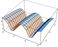
Figure 1: (a) The proper distance between two D5-branes for D3-D5 brane system given in (69) is depicted (a). It decreases monotonically as time increases. We set $M_{1}=1$, $M_{2}=1$, $c_{0}=-1$ and $L=1$. A singularity appears between two D5-branes at $t=2$ and the spacetime split into two isolated brane throats before they collide. (b) We also show the snapshots at $t=-2$ (bold),$0$ (solid), and $2$(dashed) from the top. Although the distance depends sensitively on the angle $\theta$, but not on time $t$.

Figure 2: The time change of the proper distance between two D5-branes for D3-D5 brane system at $\theta=0$ (bold), $\pi/4$ (solid) and $\pi/2$ (dashed). We choose the same parameters as Fig.1 ($M_{1}=1$, $M_{2}=1$, $c_{0}=-1$ and $L=1$). Two branes approach very slowly and a singularity appears at $t=2$.

V.2 Collision of the D$(p-2)$-D$p$ brane ($p=(8-d_{\rm Z})$)

In this case, we have one uncompactified extra dimension $z$ in ${\rm Z}$ space. Since the harmonic function $h_{1}$ is linear in $z$, we find difference behavior from the case (V.1). In order to discuss the detail, we consider one concrete example, i.e., the D3-D5 brane system which are smeared in the three transverse directions as well as ${\rm Y}$ space (see Table II).

Here we assume that D3-D5 brane system are smeared along $z^{2}$, $z^{3}$, $z^{4}$ directions. The ten-dimensional metric (48) can be written as

$$ds^{2} = \cos^{1\over 2}\theta\left(c_{0}t+h_{1}(z)\right)^{1/2}\left(\tan^{2}\theta+c_{0}t+h_{1}(z)\right)^{1/4}\left[{1\over c_{0}t+h_{1}(z)}\eta_{\mu\nu}dx^{\mu}dx^{\nu}\right.$$ (70)

$$\left.+{1\over\cos^{2}\theta\left(\tan^{2}\theta+c_{0}t+h_{1}(z)\right)}\delta_{ij}dy^{i}dy^{j}+\delta_{ab}dz^{a}dz^{b}\right]\,,$$

where we set $z=z^{1}$ and the harmonic function $h_{1}(z)$ is given by

$$h_{1}(z)=\sum_{l=1}^{N}M_{l}\,|\,z-\,z_{l}|\,.$$ (71)

We analyze the D3-D5 brane system with the brane charge $M_{1}$ at $z=0$ and the other $M_{2}$ at $z=L$. The proper distance between the two D5-branes is given by

$$d(t) = \cos^{1\over 4}\theta\int^{L}_{0}dz\left(c_{0}t+M_{1}|z|+M_{2}|z-L|\right)^{1/4}$$ (72)

$$\times\left[\tan^{2}\theta+c_{0}t+M_{1}|z|+M_{2}|z-L|\right]^{1/8}\,.$$

For $c_{0}<0$, the proper distance decreases as $t$ increases, and if $M_{1}\neq M_{2}$, a singularity appears at $t=t_{s}\equiv-[M_{1}|z|+M_{2}|z-L|]/c_{0}>0$ when the distance is still finite. This is just the same as the case in §. V.1. However, if $M_{1}=M_{2}=M$, the result changes completely. The distance eventually vanishes at $t=t_{s}:=-ML/c_{0}$ as

$$d(t)\approx\sin^{1\over 4}\theta|c_{0}|^{1\over 4}L(t_{s}-t)^{1\over 4}\propto a^{2\over 3}\,,$$ (73)

and two branes collide completely. A singularity appears at the same time. Note that the scale factor $a$ of our universe behaves as $a\propto(t_{s}-t)^{3/8}$ near collision.

We show $d(t)$ integrated numerically in Fig. 3 - Fig. 5 for the case of $c_{0}<0$.

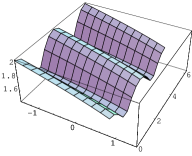
Figure 3: (a) For the case of $M_{1}\neq M_{2}$, the proper distance given in (72) is depicted. We fix $c_{0}=-1$, $M_{1}=10,M_{2}=1$ and $L=1$. (b) We also show the snapshots at $t=-1$ (thick bold), $0$ (bold), $0.5$ (solid), $0.8$ (dashed), and $1$ (dotted) from the top. Although the proper distance decreases as $t$ increases, the distance is still finite when a singularity appears at $t=1$ on the brane located at $z=0$.

In the past direction, the distance $d$ increases. Then, for $t<0$, each brane gradually separates as $|t|$ increases.

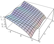
Figure 4: (a) For the case of $M_{1}=M_{2}$, the time change of the proper distance given in (72) is depicted (a). We fix $c_{0}=-1$, $M_{1}=1,M_{2}=1$ and $L=1$. The proper distance decreases as $t$ increases and it vanishes at $t=t_{s}>0$ when a singularity appears. (b) We also show the snapshots at $t=-1$ (thick bold), $0$ (bold), $0.5$ (solid), $0.8$ (dashed), and $0.99$ (dotted) from the top. $d$ vanishes at $t=1$.

Figure 5: The time change of the proper distance at $\theta=0$ (a) and $\theta=\pi/2$ (b) for $M_{1}=M_{2}=1$ and $M_{1}=10,M_{2}=1$. We fix $c_{0}=-1$, and $L=1$. The proper distance rapidly vanishes near two branes collide for the case of $M_{1}=M_{2}=1$. The dashed line denotes the case of $M_{1}=10,M_{2}=1$ while the solid one corresponds to $M_{1}=M_{2}=1$ case. While for the case of $M_{1}=10,M_{2}=1$, it is still finite when a singularity appears.

V.3 Collision of brane universes in a lower-dimensional effective theory

Next we consider the brane collision in the lower-dimensional effective theory. It is motivated by a brane world scenario, which is modeled in five dimensions after compactification brane_world0 ; brane_world1 ; brane_world2 ; brane_world3 .

We compactify the ${\rm Y}$ space and some directions of ${\rm Z}$, where D3-D5 branes have been smeared along such directions. As a result, we find the five-dimensional metric in the Einstein frame as

$$ds^{2}(\bar{{\rm M}}) = \left[c_{0}t+h_{1}(z)\right]^{1/3}\left(-dt^{2}+\delta_{pq}dx^{p}dx^{q}\right)+\left[c_{0}t+h_{1}(z)\right]^{4/3}dz^{2}\,,$$ (74)

where $h_{1}(z)$ is given by (71) . The five-dimensional metric turns out not to depend on $\theta$ , which makes some difference between analysis in full ten dimensions and that in the effective theory.

Suppose that our universe is given by D3 brane at $z=0$ and the other brane universe exists at $z=L$. The metric of our universe is given by the four-dimensional Einstein frame from the five-dimensional metric (74) as

$$ds_{4}^{2} = \left[c_{0}t+h_{1}(0)\right]\left(-dt^{2}+\delta_{pq}dx^{p}dx^{q}\right)\,,$$ (75)

where $h_{1}(0)=M_{2}L$. Introducing the cosmic time $\tau$ in four dimensions by

$${\tau_{s}-\tau\over\tau_{0}}=\left({t_{s}-t\over t_{0}}\right)^{3\over 2}\,,$$ (76)

where $t_{0}=-1/c_{0}$ and $\tau_{0}=2t_{0}/3$. $t_{s}=-M_{2}L/c_{0}$ and an integration constant $\tau_{s}$ correspond to times when a singularity appears in each time coordinate. The scale factor $a_{5}$ of our universe in the effective 5-dimensional spacetime is given by

$$a_{5}=\left({t_{s}-t\over t_{0}}\right)^{1\over 2}=\left({\tau_{s}-\tau\over\tau_{0}}\right)^{1\over 3}~{}~{}~{}~{}~{}{\rm for}~{}~{}~{}\tau<\tau_{s}\,.$$ (77)

The proper distance between two universes in this effective 5-dimensional spacetime is

$$d_{5}(t)=\left\{\begin{array}[]{ll}\displaystyle{\left({t_{s}-t\over t_{0}}\right)^{2/3}L}&~{}~{}~{}~{}{\rm for}~{}~{}M_{1}=M_{2}\\ \displaystyle{\frac{3}{5(M_{1}-M_{2})}\left[\left({t_{s}-t\over t_{0}}+(M_{1}-M_{2})L\right)^{5/3}-\left({t_{s}-t\over t_{0}}\right)^{5/3}\right]}&~{}~{}~{}~{}{\rm for}~{}~{}M_{1}\neq M_{2}\\ \end{array}\right.$$ (79)

As $t$ increases, the proper distance $d$ decreases and it eventually vanishes at $t=t_{s}\equiv ML\tau_{0}(>0)$ if $M_{1}=M_{2}=M$. When two branes approach, both universes are contracting, and a big crunch singularity appears when two branes collide. We find that a complete collision occurs simultaneously at $t=-ML/c_{0}$. The distance vanishes as $d_{5}\propto a_{5}^{4/3}$ near collision.

On the other hand, for the case of $M_{1}\neq M_{2}$, a singularity appears at at $t=t_{s}\equiv-[M_{1}|z|+M_{2}|z-L|]/c_{0}>0$, when the distance is still finite. We show $d(t)$ integrated numerically in Fig. 6.

Figure 6: The proper distance $d_{5}$ is depicted. We fix $c_{0}=-1$ and $L=1$. The proper distance decreases as $t$ increases. The bold line denotes the case of $M_{1}=10,M_{2}=1$ while the solid ones corresponds to $M_{1}=M_{2}=1$ case. If we set $M_{1}=M_{2}$, it causes the complete collision at $t=t_{s}(=1)$ simultaneously. For $M_{1}\neq M_{2}$, a singularity appears at $t=t_{s}$ when the distance is still finite. Then, the solution cannot describe collision of two branes.

We also show the comparison of the distance evaluated in the effective five dimensions and that in the original ten dimensions in Fig. 7. We find the behaviors are quite similar, i.e., two branes collide at a big crunch singularity if $M_{1}=M_{2}$, but it is not the case for $M_{1}\neq M_{2}$. However there exist quantitative differences, especially the approaching velocity of two branes in ten dimensions is much faster than that in the effective five dimensions when two branes collide ($d\propto(t_{s}-t)^{1/4}$ and $d_{5}\propto(t_{s}-t)^{2/3}$). Hence the real collision of two branes will be much more violent than that expected from the effective model.

Figure 7: The proper distance given in the effective theory is compared with that in 10-D theory ((a) $\theta=\pi/2$ (b) $\theta=0$). The bold line denotes the proper distance in the effective theory while the solid ones corresponds to the proper distance in the 10-D theory.

VI Conclusion and remarks

In this paper, we have derived the time-dependent solutions corresponding to the dynamical D-brane with angles in the ten-dimensional supergravity models and discussed their applications to cosmology and dynamics of branes. Our solutions, which have been constructed using the T-duality map between the type IIA and type IIB supergravity theories, are different from the known dynamical intersecting brane solutions in supergravity theories. These solutions are obtained by replacing a constant $c$ in the warp factor $h=c+h_{1}(z)$ of a supersymmetric static solution with a linear function of the coordinates $x^{\mu}$. This feature is shared by a wide class of supersymmetric solutions beyond the examples considered in the present paper, In the case of intersecting branes, the field equations normally indicate that time dependent solutions in supergravity can be found if only one harmonic function in the metric depends on time. However, the solutions of the intersecting brane with angles can contain two functions depending on both time as well as overall transverse space coordinates.

We then construct cosmological models from those solutions by smearing some dimensions and compactifying the internal space. We find the Friedmann-Lemaître-Robertson-Walker (FLRW) cosmological solutions with power-law expansion. Unfortunately, the power of the scale factor is so small that the solutions of field equations cannot give a realistic expansion law. The fastest expansion power is $\lambda=5/21\approx 0.238$, which is found in the case of the D3-D5 brane for the U1 type and in the D0-D2 brane system for the U2 type. This means that we have to include additional matter on the brane in order to obtain a realistic expanding universe. The properties we have discovered would also give a clue to investigate cosmological models in more complicated setup, such as D-brane with angles in the ten-dimensional string theory Breckenridge:1997ar ; Ohta:1997ku ; Ohta:1997fr ; Kitao:1998vn .

We then discuss the dynamics of branes. we have found that when the spacetime is contracting in ten dimensions, each brane approaches the others as the time evolves. All domain between branes connected initially ($t<0$), but it shrinks as the time increases. However, for the D$(p-2)$-D$p$-brane system ($p\leq 7$) without smearing branes, a singularity appears before branes collide. and eventually the topology of the spacetime changes such that parts of the branes are separated by a singular region surrounding each brane. Thus, the solution cannot describe the collision of two branes. In contrast, the D6-D8-brane system or the smeared D$(p-2)$D$p$ brane system with one uncompactified extra dimension can provide an example of colliding branes (and collision of the universes), if they have the same charges.

We also our results in ten-dimensional spacetime and those in the effective five-dimensional theory. Although the present models allow the Kaluza-Klein compactification, i.e., the dynamics is still correct in the effective theory, the behavior of collision looks different. The collision in ten dimensions is more violent than that in the effective five dimensions. It is just because the definitions of the distances are different. Hence we have to careful to analyze our results obtained in the effective theory.

Although the present examples illustrated in the this paper provide neither realistic cosmological model nor collision of branes (or of the universes), the features of the solutions or the method to obtain them could open new directions to study how to construct a realistic dynamics of branes as well as an appropriate higher-dimensional cosmological model.

Appendix A Dynamical brane in massive supergravity

In this appendix, we will derive another time dependent solution for D6-D8 brane system.

The action for the massive IIA supergravity in the Einstein frame can be written as Singh:2001gt ; Singh:2002eu

$$S = \frac{1}{2\kappa^{2}}\int\left(R\ast{\bf 1}-\frac{1}{2}d\phi\wedge\ast d\phi-\frac{1}{2\cdot 2!}{\rm e}^{3\phi/2}F_{(2)}\wedge\ast F_{(2)}-\frac{1}{2\cdot 3!}{\rm e}^{-\phi}H_{(3)}\wedge\ast H_{(3)}\right.$$ (80)

$$\left.-\frac{1}{2\cdot 4!}{\rm e}^{\phi/2}\bar{F}_{(4)}\wedge\ast\bar{F}_{(4)}-\frac{1}{2}{\rm e}^{5\phi/2}m_{0}^{2}\ast{\bf 1}-\frac{1}{2}B_{(2)}\wedge\bar{F}_{(4)}\wedge\bar{F}_{(4)}\right)\,,$$

where $\kappa^{2}$ is the ten-dimensional gravitational constant, $m_{0}$ is constant, $\ast$ is the Hodge dual operator in the ten-dimensional spacetime, and $F_{(2)}$, $H_{(3)}$, $\bar{F}_{(4)}$ are 2-form, 3-form, 4-form field strength, respectively. The expectation values of fermionic fields are assumed to vanish. The field strengths in the action (80) are given by

$$H_{(3)} = dB_{(2)}\,,$$ (81a)

$$F_{(2)} = dC_{(1)}+m_{0}B_{(2)}\,,$$ (81b)

$$F_{(4)} = \bar{F}_{(4)}+C_{(1)}\wedge H_{(3)}\,,$$ (81c)

$$\bar{F}_{(4)} = dC_{(3)}+m_{0}B_{(2)}\wedge B_{(2)}\,,$$ (81d)

where $C_{(1)}$, $B_{(2)}$, $C_{(3)}$ are 1-form, 2-form, 3-form, respectively.

After variations with respect to the metric, the scalar field, and the gauge field, the field equations of the D6-D8 brane system can be written by

$$R_{MN}=\frac{1}{2}\partial_{M}\phi\partial_{N}\phi+\frac{1}{16}{\rm e}^{5\phi/2}m_{0}^{2}+\frac{1}{2\cdot 2!}{\rm e}^{3\phi/2}\left(2F_{MA}{F_{N}}^{A}-\frac{1}{8}g_{MN}F_{(2)}^{2}\right)$$

$$\hskip 42.67912pt+\frac{1}{2\cdot 3!}{\rm e}^{-\phi}\left(3H_{MAB}{H_{N}}^{AB}-\frac{1}{4}g_{MN}H_{(3)}^{2}\right)\,,$$ (82a)

$$d\ast d\phi=\frac{3}{4\cdot 2!}{\rm e}^{3\phi/2}F_{(2)}\wedge\ast F_{(2)}-\frac{1}{2\cdot 3!}{\rm e}^{-\phi}H_{(3)}\wedge\ast H_{(3)}+\frac{1}{2}{\rm e}^{5\phi/2}m_{0}^{2}\ast{\bf 1}\,,$$ (82b)

$$d\left({\rm e}^{3\phi/2}\ast F_{(2)}\right)=0\,,$$ (82c)

$$d\left({\rm e}^{-\phi}\ast H_{(3)}\right)+m_{0}\,{\rm e}^{3\phi/2}\ast F_{(2)}=0\,.$$ (82d)

To solve the field equations, we assume the ten-dimensional metric in the form

$$ds^{2} = h_{\theta}^{1/4}(x,z)h^{7/8}(x,z)\left[h^{-1}(x,z)q_{\mu\nu}({\rm X})dx^{\mu}dx^{\nu}+h_{\theta}^{-1}(x,z)u_{ij}({\rm Y})dy^{i}dy^{j}+dz^{2}\right]\,,~{}~{}~{}~{}$$ (83)

where $q_{\mu\nu}$ is a seven-dimensional metric which depends only on the seven-dimensional coordinates $x^{\mu}$, and $u_{ij}$ is the two-dimensional metric which depends only on the two-dimensional coordinates $y^{i}$, and the function $h_{\theta}$ is given by

$$h_{\theta}=1+\cos^{2}\theta\left(h-1\right)\,.$$ (84)

The metric form (83) is a straightforward generalization of the case of a static D6-D8 brane system with a dilaton coupling Singh:2002eu . Furthermore, we assume that the scalar field $\phi$, the parameter $m_{0}$ and the gauge field strengths are given by

$${\rm e}^{\phi} = h_{\theta}^{-1/2}h^{-3/4},$$ (85a)

$$B_{(2)} = \tan\theta\left(h_{\theta}^{-1}-1\right)\Omega({\rm Y})\,,$$ (85b)

$$dC_{(1)} = m\sin\theta\,\Omega({\rm Y})\,,$$ (85c)

$$m = m_{0}\left(\cos\theta\right)^{-1}\,,$$ (85d)

where $\Omega({\rm Y})$ denotes the volume 2-form,

$$\Omega({\rm Y}) = \sqrt{u}\,dy^{1}\wedge dy^{2}\,.$$ (86)

The assumptions on the ten-dimensional metric and fields correspond to the following brane configuration:

	0	1	2	3	4	5	6	7	8	9
D6	$\circ$	$\circ$	$\circ$	$\circ$	$\circ$	$\circ$	$\circ$
D8	$\circ$	$\circ$	$\circ$	$\circ$	$\circ$	$\circ$	$\circ$	$\circ$	$\circ$
$X^{A}$	$~{}t~{}$	$x^{1}$	$x^{2}$	$x^{3}$	$x^{4}$	$x^{5}$	$x^{6}$	$y^{1}$	$y^{2}$	$~{}z~{}$

Let us first consider the Einstein equations (82a). Using the assumptions (83) and (85), the Einstein equations are given by

$$R_{\mu\nu}({\rm X})-h^{-1}D_{\mu}D_{\nu}h+\frac{1}{16}q_{\mu\nu}h^{-1}\left(\Box_{{\rm X}}h+h^{-1}\partial_{z}^{2}h\right)-\frac{1}{8}q_{\mu\nu}h_{\theta}^{-1}\left(\Box_{{\rm X}}h_{\theta}+h^{-1}\partial_{z}^{2}h_{\theta}\right)$$

$$+\frac{1}{16}h^{-3}h_{\theta}^{-1}\left(h_{\theta}-2\sin^{2}\theta\right)\left[\left(\partial_{z}h\right)^{2}-m^{2}\right]=0\,,$$ (87a)

$$\partial_{\mu}\partial_{z}h=0\,,$$ (87b)

$$R_{ij}({\rm Y})-\frac{7}{16}u_{ij}h_{\theta}^{-1}\left(\Box_{{\rm X}}h+h^{-1}\partial_{z}^{2}h\right)+\frac{3}{8}u_{ij}hh_{\theta}^{-1}\left(\Box_{{\rm X}}h_{\theta}+h^{-1}\partial_{z}^{2}h_{\theta}\right)$$

$$+\frac{1}{16}h^{-2}h_{\theta}^{-3}\left(h_{\theta}^{3}+6\sin^{2}\theta\right)\left[\left(\partial_{z}h\right)^{2}-m^{2}\right]=0\,,$$ (87c)

$$-\frac{7}{16}\left(\Box_{{\rm X}}h+h^{-1}\partial_{z}^{2}h\right)-\frac{1}{8}hh_{\theta}^{-1}\left(\Box_{{\rm X}}h_{\theta}+h^{-1}\partial_{z}^{2}h_{\theta}\right)+\frac{1}{16}h^{-2}\left[\left(\partial_{z}h\right)^{2}-m^{2}\right]=0\,,$$ (87d)

where $D_{\mu}$ is the covariant derivative with respective to the metric $q_{\mu\nu}$, $\Box_{{\rm X}}$ is the Laplace operator on the space of ${\rm X}$, and $R_{\mu\nu}({\rm X})$, $R_{ij}({\rm Y})$ are the Ricci tensors of the metrics $q_{\mu\nu}({\rm X})$, $u_{ij}({\rm Y})$, respectively.

From Eq. (87b), the warp factor $h$ must be in the form

$$h(x,z)=K_{0}(x)+K_{1}(z)\,.$$ (88)

With this form of $h$, the other components of the Einstein equations (87) are rewritten as

$$R_{\mu\nu}({\rm X})-h^{-1}D_{\mu}D_{\nu}K_{0}+\frac{1}{16}q_{\mu\nu}h^{-1}\left(\Box_{{\rm X}}K_{0}+h^{-1}\partial_{z}^{2}K_{1}\right)-\frac{1}{8}q_{\mu\nu}h_{\theta}^{-1}\left(\Box_{{\rm X}}K_{0}+h^{-1}\partial_{z}^{2}K_{1}\right)$$

$$+\frac{1}{16}h^{-3}h_{\theta}^{-1}\left(h_{\theta}-2\sin^{2}\theta\right)\left[\left(\partial_{z}K_{1}\right)^{2}-m^{2}\right]=0\,,$$ (89a)

$$R_{ij}({\rm Y})-\frac{7}{16}u_{ij}h_{\theta}^{-1}\left(\Box_{{\rm X}}K_{0}+h^{-1}\partial_{z}^{2}K_{1}\right)+\frac{3}{8}\cos^{2}\theta u_{ij}hh_{\theta}^{-1}\left(\Box_{{\rm X}}K_{0}+h^{-1}\partial_{z}^{2}K_{1}\right)$$

$$+\frac{1}{16}h^{-2}h_{\theta}^{-3}\left(h_{\theta}^{3}+6\sin^{2}\theta\right)\left[\left(\partial_{z}K_{1}\right)^{2}-m^{2}\right]=0\,,$$ (89b)

$$-\frac{7}{16}\left(\Box_{{\rm X}}K_{0}+h^{-1}\partial_{z}^{2}K_{1}\right)-\frac{1}{8}hh_{\theta}^{-1}\left(\Box_{{\rm X}}K_{0}+h^{-1}\partial_{z}^{2}K_{1}\right)+\frac{1}{16}h^{-2}\left[\left(\partial_{z}K_{1}\right)^{2}-m^{2}\right]=0\,.~{}~{}~{}$$ (89c)

Let us next consider the 2-form field $B_{(2)}$ and 1-form $A_{(1)}$. Under the assumption (85), the equation of motion for the gauge field $B$ becomes

$$\sin 2\theta\left[\left(\Box_{{\rm X}}K_{0}+h^{-1}\partial_{z}^{2}K_{1}\right)-h^{-2}\left\{\left(\partial_{z}K_{1}\right)^{2}-m^{2}\right\}\right]\Omega({\rm X})\wedge dz=0\,,$$ (90)

where we used Eq. (88). Then, for $\sin 2\theta\neq 0$, Eq. (90) is reduced to

$$\Box_{{\rm X}}K_{0}=0\,,~{}~{}~{}\partial_{z}K_{1}=\pm m\,.$$ (91)

Eq. (91) thus gives

$$K_{1}(z)=1\pm mz\,.$$ (92)

Eq. (90) is automatically satisfied for $\sin 2\theta=0$. Let us next consider the scalar field equation. Substituting the forms of the function $h$ (88) into the equation of motion for the scalar field (82b), we obtain

$$\left(5h_{\theta}-2\sin^{2}\theta\right)\left[h^{2}\Box_{{\rm X}}K_{0}+h_{\theta}\left\{\left(\partial_{z}K_{1}\right)^{2}-m^{2}\right\}\right]=0\,.$$ (93)

Thus, the warp factor $h$ should satisfy Eq. (91). Then, the Einstein equations reduce to

$$R_{\mu\nu}({\rm X})=0\,,$$ (94a)

$$R_{ij}({\rm Y})=0\,,$$ (94b)

$$h(x,z)=K_{0}(x)+K_{1}(z)\,;~{}~{}D_{\mu}D_{\nu}K_{0}=0\,,~{}~{}K_{1}(z)=1\pm mz\,.$$ (94c)

As a special example, we consider the case

$$q_{\mu\nu}=\eta_{\mu\nu}\,,\quad u_{ij}=\delta_{ij}\,,$$ (95)

where $\eta_{\mu\nu}$ is the seven-dimensional Minkowski metric and $\delta_{ij}$ is the two-dimensional Euclidean metric. In this case, the solution for $h$ can be obtained explicitly as

$$h(x,z)=c_{\mu}x^{\mu}\pm m(z-z_{0})\,,$$ (96)

where $c_{\mu}$ and $z_{0}$ are constant parameters.

Here we shall discuss the case of $p=8$. It provides us a colliding-brane model in a massive supergravity. It may capture the essence of brane collision. The dynamical D8-brane solution is written as

$$ds^{2} = \cos^{1\over 2}\theta\left[c_{0}t+\sum_{l}M_{l}|z-z_{l}|\right]^{7/8}\left[c_{0}t+\sum_{l}M_{l}|z-z_{l}|+\tan^{2}\theta\right]^{1/4}$$ (97)

$$\times\left[{1\over c_{0}t+\sum_{l}M_{l}|z-z_{l}|}\,\eta_{\mu\nu}dx^{\mu}dx^{\nu}\right.$$

$$\left.~{}~{}~{}+{1\over\cos^{2}\theta\left[c_{0}t+\sum_{l}M_{l}|z-z_{l}|+\tan^{2}\theta\right]}\,\delta_{ij}dy^{i}dy^{j}+\delta_{ab}dz^{a}dz^{b}\right]\,,$$

where the constant $\,z_{l}$ denotes the position of the D8-brane with charge $M_{l}$.

Let us consider the two D8-branes with the brane charge $M_{1}$ at $z=0$ and the other $M_{2}$ at $z=L$. The proper distance between two D8-branes is given by

$$d(t)=\cos^{1\over 4}\theta\int^{L}_{0}dz\left(c_{0}t+M_{1}|z|+M_{2}|z-L|\right)^{\frac{7}{16}}\left(c_{0}t+M_{1}|z|+M_{2}|z-L|+\tan^{2}\theta\right)^{\frac{1}{8}}\,.~{}~{}~{}~{}$$ (98)

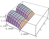
Figure 8: The proper distance given in (98) is depicted. We fix $c_{0}=-1$ and $L=1$. The proper distance decreases as $t$ increases. If two D8-brane satisfy $M_{1}=M_{2}$, it causes the complete collision at $t=1$ simultaneously. For $M_{1}\neq M_{2}$, a singularity appears at $t=t_{s}>0$ when the distance is still finite. Then, the solution does not describe the collision of two D8-branes.

For $c_{0}<0$, the proper distance decreases as $t$ increases, and it eventually vanishes at $t=-ML/c_{0}$ if two brane charges are equal such that $M_{1}=M_{2}=M$. Hence, one D8-brane approaches the other as time progresses, causing the complete collision at $t=-ML/c_{0}$. We note that the collision occurs simultaneously. This behavior, however, changes if $M_{1}\neq M_{2}$. A singularity forms at $t=t_{s}\equiv-[M_{1}|z|+M_{2}|z-L|]/c_{0}>0$, when the distance is still finite. We show $d(t)$ in Fig. 8.

For $t<0$, each brane gradually separates from the other as the time goes in the past.

Appendix B D0-D2-D2-D4 brane system

In this appendix, we discuss the solution for involving more than two types of D-branes. This is given by the procedure of delocalization, rotation and T duality with respect to more than one of the transverse coordinates of the original D-brane solutions. Let us consider the D0-D2-brane with D4-brane system. The ten-dimensional metric is given by Breckenridge:1996tt

$$ds^{2} = h^{1/8}(t,z)h_{\theta}^{1/4}(t,z)h_{\psi}^{1/4}(t,z)\left[-h^{-1}(t,z)dt^{2}+h_{\theta}^{-1}(t,z)\gamma_{ij}({\rm Y}_{1})dy^{i}dy^{j}\right.$$ (99)

$$\left.+h_{\psi}^{-1}(t,z)v_{mn}({\rm Y}_{2})d\eta^{m}d\eta^{n}+u_{ab}({\rm Z})dz^{a}dz^{b}\right]\,,$$

where $\gamma_{ij}$ is the two-dimensional metric which depends only on the two-dimensional coordinates $y^{i}$, $v_{mn}$ is the two-dimensional metric which depends only on the two-dimensional coordinates $\eta^{m}$, and $u_{ab}$ is the five-dimensional metric which depends only on the five-dimensional coordinates $z^{a}$, and the functions $h_{\theta}$, $h_{\psi}$ are given by

$$h_{\theta}(t,z)=1+\cos^{2}\theta\left(h-1\right)\,,~{}~{}~{}~{}h_{\psi}(t,z)=1+\cos^{2}\psi\left(h-1\right)\,.$$ (100)

The assumptions on the ten-dimensional metric and fields correspond to the following brane configuration:

	0	1	2	3	4	5	6	7	8	9
D0	$\circ$
D2	$\circ$	$\circ$	$\circ$
D2	$\circ$			$\circ$	$\circ$
D4	$\circ$	$\circ$	$\circ$	$\circ$	$\circ$
$X^{A}$	$~{}t~{}$	$y^{1}$	$y^{2}$	$\eta^{1}$	$\eta^{2}$	$z^{1}$	$z^{2}$	$z^{3}$	$z^{4}$	$z^{5}$

The scalar field $\phi$ and the gauge field strengths are given by

$${\rm e}^{\phi} = h^{3/4}\left(h_{\theta}h_{\psi}\right)^{-1/2}\,,$$ (101a)

$$C_{(1)} = \pm\sin\theta\sin\psi\left(h^{-1}-1\right)dt\,,$$ (101b)

$$C_{(3)} = \pm\cos^{-1}\theta\sin\psi\left(h_{\theta}^{-1}-1\right)dt\wedge\Omega({\rm Y}_{1})$$ (101c)

$$\pm\cos^{-1}\psi\sin\theta\left(h_{\psi}^{-1}-1\right)dt\wedge\Omega({\rm Y}_{2})+\omega_{(3)}\,,$$

$$B_{(2)} = \tan\theta\,\left(h_{\theta}^{-1}-1\right)\Omega({\rm Y}_{1})+\tan\psi\,\left(h_{\psi}^{-1}-1\right)\Omega({\rm Y}_{2})\,,$$ (101d)

where $\Omega({\rm Y}_{1})$ and $\Omega({\rm Y}_{2})$ denote the volume form,

$$\Omega({\rm Y}_{1})=\sqrt{\gamma}\,dy^{1}\wedge dy^{2}\,,~{}~{}~{}~{}\Omega({\rm Y}_{2})=\sqrt{v}\,d\eta^{1}\wedge d\eta^{2}\,,$$ (102)

and the three form $\omega_{(3)}$ satisfies

$$d\omega_{(3)}=\pm\cos\theta\,\cos\psi\,\partial_{a}h\ast_{{\rm Z}}\left(dz^{a}\right)\,.$$ (103)

Here $\ast_{{\rm Z}}$ denotes the Hodge operator on ${\rm Z}$.

Performing the same procedure as in the previous section, we find that the field equations are reduced to

$$R_{ij}({\rm Y}_{1})=0\,,$$ (104a)

$$R_{mn}({\rm Y}_{2})=0\,,$$ (104b)

$$R_{ab}({\rm Z})=0\,,$$ (104c)

$$h(t,z)=K_{0}(t)+K_{1}(z);~{}~{}~{}\partial_{t}^{2}K_{0}=0\,,~{}~{}~{}{\triangle}_{{\rm Z}}K_{1}=0\,,$$ (104d)

$$h_{\theta}(t,z)=1+\cos^{2}\theta(h-1)\,,~{}~{}~{}~{}h_{\psi}(t,z)=1+\cos^{2}\psi(h-1)\,,$$ (104e)

where $\triangle_{{\rm Z}}$ is the Laplace operators on the space of ${\rm Z}$, and $R_{ij}({\rm Y}_{1})$, $R_{mn}({\rm Y}_{2})$, and $R_{ab}({\rm Z})$ are the Ricci tensors of the metrics $\gamma_{ij}({\rm Y}_{1})$, $v_{mn}({\rm Y}_{2})$, and $u_{ab}({\rm Z})$, respectively.

Let us consider the case $u_{ab}=\delta_{ab}$ in more detail, where $\delta_{ab}$ are the five-dimensional Euclidean metric. In this case, a solution for the warp factor $h$ can be obtained explicitly as

$$h(t,z)=ct+\tilde{c}+\sum_{l}\frac{M_{l}}{|z^{a}-z^{a}_{l}|^{3}}\,,$$ (105)

where $c$, $\tilde{c}$, $M_{l}$ and $z_{l}$ are constant parameters.

If the branes exist at the origin of ${\rm Z}$ space, introducing a radial coordinate $r$ by

$$\delta_{ab}dz^{a}dz^{b}=dr^{2}+r^{2}d\Omega^{2}_{4}\,,$$ (106)

we find that the function $h$ is expressed as

$$h=c_{0}t+\tilde{c}+\left(\frac{m}{r}\right)^{3}\,,$$ (107)

where $d\Omega^{2}_{4}$ is the line element of four-dimensional sphere, and $c_{0}$, $\tilde{c}$, and $m$ are constants. In the limit $r\rightarrow 0$, the metric (99) gives

$$ds^{2} = \left(\cos\theta\cos\psi\right)^{1/2}\left(\frac{m}{r}\right)^{-1/8}\left[\left(\frac{m}{r}\right)^{-1}\left(-dt^{2}+\cos^{-2}\theta\gamma_{ij}dy^{i}dy^{j}+\cos^{-2}\psi v_{mn}d\eta^{m}d\eta^{n}\right)\right.$$ (108)

$$\left.+m^{2}\frac{dr^{2}}{r^{2}}+m^{2}d\Omega_{4}^{2}\right]\,,$$

while the dilaton is given by

$$\lim_{r\rightarrow 0}{\rm e}^{\phi}=\left(\cos\theta\cos\psi\right)^{-1}\left(\frac{m}{r}\right)^{-3/4}\,.$$ (109)

Hence the ten-dimensional metric with $\theta=0$, $\psi=0$, $\gamma_{ij}=\delta_{ij}$, and $v_{mn}=\delta_{mn}$ becomes a warped ${\rm AdS}_{6}\times{\rm S}^{4}$ spacetime.

The dynamical solution can be obtained by the same procedure of the delocalization and rotation on a D2-brane. Let us single out two orthogonal planes $(y^{1},y^{2})$ and $(\eta^{1},\eta^{2})$. If we apply the procedure of the delocalization and rotation on a D2-brane with respect to the $(y^{1},y^{2})$ plane, followed by T-duality map (37), we can obtain the solution for a D3-D1 brane, where the rotation angle is given by $\theta$. After repeating the same procedure of the delocalization and rotation on a D3-brane with respect to the $(\eta^{1},\eta^{2})$ plane - rotating by $\psi$ to $(\eta^{1},\eta^{2})$ - , followed by T-duality map Bergshoeff:1995as ; Breckenridge:1997ar

$$g^{(\rm A)}_{yy}=\frac{1}{g^{(\rm B)}_{yy}}\,,~{}~{}~{}~{}g^{(\rm A)}_{\mu\nu}=g^{(\rm B)}_{\mu\nu}-\frac{g^{(\rm B)}_{y\mu}g^{(\rm B)}_{y\nu}-B^{(\rm B)}_{y\mu}B^{(\rm B)}_{y\nu}}{g^{(\rm B)}_{yy}}\,,~{}~{}~{}~{}g^{(\rm A)}_{y\mu}=-\frac{B^{(\rm B)}_{y\mu}}{g^{(\rm B)}_{yy}}\,,$$

$${\rm e}^{2\phi_{(\rm A)}}=\frac{{\rm e}^{2\phi_{(\rm B)}}}{g^{(\rm B)}_{yy}}\,,~{}~{}~{}~{}C_{\mu}=C_{y\mu}+C_{(0)}B_{y\mu}^{(\rm B)}\,,~{}~{}~{}~{}C_{y}=-C_{(0)}\,,$$

$$B^{(\rm A)}_{\mu\nu}=B^{(\rm B)}_{\mu\nu}+2\frac{B^{(\rm B)}_{y[\mu}\,g^{(\rm B)}_{\nu]y}}{g^{(\rm B)}_{yy}}\,,~{}~{}~{}~{}B^{(\rm A)}_{y\mu}=-\frac{g^{(\rm B)}_{y\mu}}{g^{(\rm B)}_{yy}}\,,~{}~{}~{}~{}C_{y\mu\nu}=C_{\mu\nu}+2\frac{C_{y[\mu}\,g^{(\rm B)}_{\nu]y}}{g^{(\rm B)}_{yy}}\,,$$

$$C_{\mu\nu\rho}=C_{\mu\nu\rho y}+\frac{3}{2}\left(C_{y[\mu}\,B^{(\rm B)}_{\nu\rho]}-B^{(\rm B)}_{y[\mu}\,C_{\nu\rho]}-4\frac{B^{(\rm B)}_{y[\mu}\,C_{|y|\nu}g^{(\rm B)}_{\rho]y}}{g^{(\rm B)}_{yy}}\right)\,,$$ (110)

we can construct the solution of the D0-D2-D4-brane system (105) Breckenridge:1996tt . Here $y$ is the coordinate to which the T dualization is applied, and $\mu$, $\nu$, and $\rho$ denote the coordinates other than $y$.

By smearing ${\rm Y}_{1}$ space, ${\rm Y}_{2}$ space, and some of ${\rm Z}$ space ( $0\leq d_{\rm Z}\leq 2$ dimensions)and compactifying them, we can construct the type U2 isotropic and homogeneous three space as our universe. We can also discuss collision of branes (or universes).

References

(1)
G. W. Gibbons, H. Lu and C. N. Pope,
Phys. Rev. Lett. 94 (2005) 131602
[arXiv:hep-th/0501117].
(2)
W. Chen, Z. W. Chong, G. W. Gibbons, H. Lu and C. N. Pope,
Nucl. Phys. B 732 (2006) 118
[arXiv:hep-th/0502077].
(3)
H. Kodama and K. Uzawa,
JHEP 0507 (2005) 061
[arXiv:hep-th/0504193].
(4)
P. Binetruy, M. Sasaki and K. Uzawa,
Phys. Rev. D 80 (2009) 026001
[arXiv:0712.3615 [hep-th]].
(5)
K. Maeda, N. Ohta, M. Tanabe and R. Wakebe,
JHEP 0906 (2009) 036
[arXiv:0903.3298 [hep-th]].
(6)
K. Maeda, N. Ohta and K. Uzawa,
JHEP 0906 (2009) 051
[arXiv:0903.5483 [hep-th]].
(7)
G. W. Gibbons and K. Maeda,
Phys. Rev. Lett. 104 (2010) 131101
[arXiv:0912.2809 [gr-qc]].
(8)
K. Maeda and M. Nozawa,
Phys. Rev. D 81 (2010) 044017
[arXiv:0912.2811 [hep-th]].
(9)
K. Maeda, N. Ohta, M. Tanabe and R. Wakebe,
JHEP 1004 (2010) 013
[arXiv:1001.2640 [hep-th]].
(10)
K. Maeda and M. Nozawa,
Phys. Rev. D 81 (2010) 124038
[arXiv:1003.2849 [gr-qc]].
(11)
M. Minamitsuji, N. Ohta and K. Uzawa,
Phys. Rev. D 81 (2010) 126005
[arXiv:1003.5967 [hep-th]].
(12)
K. Maeda, M. Minamitsuji, N. Ohta and K. Uzawa,
Phys. Rev. D 82 (2010) 046007
[arXiv:1006.2306 [hep-th]].
(13)
M. Minamitsuji, N. Ohta and K. Uzawa,
Phys. Rev. D 82 (2010) 086002
[arXiv:1007.1762 [hep-th]].
(14)
M. Minamitsuji and K. Uzawa,
Phys. Rev. D 83 (2011) 086002
[arXiv:1011.2376 [hep-th]].
(15)
K. i. Maeda and M. Nozawa,
Prog. Theor. Phys. Suppl. 189 (2011) 310
[arXiv:1104.1849 [hep-th]].
(16)
M. Minamitsuji and K. Uzawa,
Phys. Rev. D 84 (2011) 126006
[arXiv:1109.1415 [hep-th]].
(17)
N. Arkani-Hamed, S. Dimopoulos, G. Dvali, Phys. Lett. B429, 263 (1998) [hep-ph/9803315];
I. Antoniadis, N. Arkani-Hamed, S. Dimopoulos, G. Dvali, Phys. Lett. B436, 257 (1998) [hep-ph/9804398];
I. Antoniadis, Phys. Lett. B246, 377 (1990).
See also: K. Akama, Lect. Notes Phys. 176, 267 (1982) [hep-th/0001113];
V. Rubakov, M.E. Shaposhnikov, Phys. Lett. B125, 136 (1983);
M. Visser, Phys. Lett. B159, 22 (1985) [hep-th/9910093];
G.W. Gibbons, D.L. Wiltshire, Nucl. Phys. B287, 717 (1987) [hep-th/0109093];
M. Gogberashvili, Europhys. Lett. 49, 396 (2000) [hep-ph/9812365].
(18)
L. Randall and R. Sundrum, Phys. Rev. Lett. 83 (1999) 3370;
ibid. 4690:
(19)
P. Binetruy, C. Deffayet, and D. Langlois, Nucl. Phys. B565 (2000) 269;
C. Csaki, M. Graesser, C. Kold, and J. Terning, Phys. Lett. B
462 (1999) 34;
J.M. Cline, C. Grojean, and G. Servant, Phys. Rev. Lett. 83 (1999) 4245;
M. Cvetic and H. Soleng, Phys. Rep. 282 (1997) 159; K.
Behrndt and M. Cvetic, Phys. Lett. B 475 (2000) 253.
(20)
T. Shiromizu, K. Maeda, and M. Sasaki,
PhysRev D.62 (2000)024012.
(21)
G.R. Dvali and S.-H.H. Tye,
Phys. Lett. B 450, 72 (1999)
[arXiv;hep-th/9812483];
S.B. Giddings, S. Kachru and J. Polchinski,
Phys. Rev. D 66, 106006 (2002)
[arXiv:hep-th/0105097];
S. Kachru, R. Kallosh, A. Linde, and S.P. Trivedi,
Phys. Rev. D 68, 046005 (2003)
[arXiv:hep-th/0301240];
S. Kachru, R. Kallosh, A. Linde, J. Maldacena, L. McAllister and S.P. Trivedi,
JCAP 0310 (2003) 013,
[arXiv:hep-th/0308055].
See also the following review article:
S.-H.H. Tye
Lect. Notes Phys. 737, 949 (2008)
[arXiv:hep-th/0610221v2].
(22)
K. Maeda, Prog.Theor.Phys.Suppl.172 (2008) 90.
Dynamics of colliding branes and black brane production.
Y. Takamizu, H. Kudoh, K. Maeda,
Phys.Rev.D7̱5(2007) 061304.
G. Gibbons,.K. Maeda, Y. Takamizu,
Phys.Lett.B647 (2007) 1.
Y. Takamizu, K. Maeda, Phys.Rev.D73 (2006) 103508.
Y. Takamizu, K. Maeda, Phys.Rev.D70 (2004) 123514.
(23)
J. Khoury, B. A. Ovrut, P. J. Steinhardt and N. Turok, Phys. Rev. D 64
(2001)123522.
P.J. Steinhardt and N. Turok, Science 296(2002) 1436 ;
P.J. Steinhardt and N. Turok, Phys. Rev. D 65 (2002) 126003.
See also the following review article: N. Turok and P.J. Steinhardt
Phys. Scr. 2005 (2005) 76.
(24)
H. Kodama and K. Uzawa,
JHEP 0603 (2006) 053
[arXiv:hep-th/0512104].
(25)
J. C. Breckenridge, G. Michaud and R. C. Myers,
Phys. Rev. D 55 (1997) 6438
[arXiv:hep-th/9611174].
(26)
D. Youm,
Phys. Rept. 316 (1999) 1
[arXiv:hep-th/9710046].
(27)
P. Di Vecchia, M. Frau, A. Lerda and A. Liccardo,
Nucl. Phys. B 565 (2000) 397
[arXiv:hep-th/9906214].
(28)
P. Di Vecchia and A. Liccardo,
NATO Adv. Study Inst. Ser. C. Math. Phys. Sci. 556 (2000) 1
[arXiv:hep-th/9912161].
(29)
P. Di Vecchia and A. Liccardo,
arXiv:hep-th/9912275.
(30)
J. M. Maldacena and J. G. Russo,
JHEP 9909 (1999) 025
[arXiv:hep-th/9908134].
(31)
J. X. Lu and S. Roy,
Nucl. Phys. B 579 (2000) 229
[arXiv:hep-th/9912165].
(32)
J. X. Lu, S. Roy and H. Singh,
JHEP 0009 (2000) 020
[arXiv:hep-th/0006193].
(33)
R. G. Cai and N. Ohta,
Phys. Rev. D 61 (2000) 124012
[arXiv:hep-th/9910092].
(34)
R. G. Cai and N. Ohta,
JHEP 0003 (2000) 009
[arXiv:hep-th/0001213].
(35)
R. G. Cai and N. Ohta,
Prog. Theor. Phys. 104 (2000) 1073
[arXiv:hep-th/0007106].
(36)
S. Kachru, R. Kallosh, A. D. Linde and S. P. Trivedi,
Phys. Rev. D 68 (2003) 046005
[arXiv:hep-th/0301240].
(37)
S. Kachru, R. Kallosh, A. D. Linde, J. M. Maldacena, L. P. McAllister and S. P. Trivedi,
JCAP 0310 (2003) 013
[arXiv:hep-th/0308055].
(38)
E. Silverstein,
Phys. Rev. D 77 (2008) 106006
[arXiv:0712.1196 [hep-th]].
(39)
E. Bergshoeff, C. M. Hull and T. Ortin,
Nucl. Phys. B 451 (1995) 547
[arXiv:hep-th/9504081].
(40)
J. C. Breckenridge, G. Michaud and R. C. Myers,
Phys. Rev. D 56 (1997) 5172
[arXiv:hep-th/9703041].
(41)
N. Ohta and J. G. Zhou,
Phys. Lett. B 418 (1998) 70
[arXiv:hep-th/9709065].
(42)
N. Ohta and P. K. Townsend,
Phys. Lett. B 418 (1998) 77
[arXiv:hep-th/9710129].
(43)
T. Kitao, N. Ohta and J. G. Zhou,
Phys. Lett. B 428 (1998) 68
[arXiv:hep-th/9801135].
(44)
H. Singh,
JHEP 0204 (2002) 017
[arXiv:hep-th/0109147].
(45)
H. Singh,
Nucl. Phys. B 661 (2003) 394
[arXiv:hep-th/0212103].