The Galaxy Optical Luminosity Function from the AGN and Galaxy Evolution Survey (AGES)

Abstract

We present the galaxy optical luminosity function for the redshift range $0.05<z<0.75$ from the AGN and Galaxy Evolution Survey (AGES), a spectroscopic survey of 7.6 deg² in the Boötes field of the NOAO Deep Wide-Field Survey. Our statistical sample is comprised of 12,473 galaxies with known redshifts down to $I=20.4$ (AB). Our results at low redshift are consistent with those from SDSS; at higher redshift, we find strong evidence for evolution in the luminosity function, including differential evolution between blue and red galaxies. We find that the luminosity density evolves as $(1+z)^{(0.54\pm 0.64)}$ for red galaxies and $(1+z)^{(1.64\pm 0.39)}$ for blue galaxies.

1. Introduction

The galaxy luminosity function directly quantifies the total light in galaxies, and its evolution characterizes the growth of galaxies over cosmic time either through star formation or hierarchical assembly. Since the first systematic galaxy redshift surveys in the 1980s (Huchra et al., 1983), the volume of the universe probed by uniform imaging and the number of galaxies with known redshifts have grown exponentially. With the advent of large, homogeneous, imaging and spectroscopic surveys of the nearby universe, such as the Two Degree Field Galaxy Redshift Survey (2dF; Colless et al., 2001) and the Sloan Digital Sky Survey (SDSS; York et al., 2000) as well as large-scale photometric redshift surveys such as COMBO17 (Wolf et al., 2003), the local ($z<0.2$) galaxy optical luminosity function is quite well constrained near $L_{*}$ (e.g., Blanton et al., 2001; Kochanek et al., 2001; Madgwick et al., 2002; Norberg et al., 2002; Blanton et al., 2003; Bell et al., 2004; Croton et al., 2005; Montero-Dorta & Prada, 2009).

In order to measure the evolution in the field galaxy luminosity function, one requires measurements at several redshifts. With the advent of more powerful telescopes and instrumentation, a number of pencil beam surveys were used to quantify the galaxy luminosity density beyond $z=0.5$ (e.g, Lilly et al., 1995; Cowie et al., 1996; Brinchmann et al., 1998; Lin et al., 1999; Cohen, 2002; Im et al., 2002; de Lapparent et al., 2003; Cross et al., 2004; Pozzetti et al., 2003). These pencil beam surveys, however, often probe volumes too small to be representative of the entire galaxy population (i.e. cosmic variance). Recently, several larger area surveys, targeting many thousands of galaxies to $z\sim 1$, have allowed for more robust statistics of the high-redshift luminosity function. The VIMOS/VVDS Deep Survey (VVDS; Le Fèvre et al., 2004) has measured the evolution of the total galaxy luminosity function to $z\sim 1.2$ with a sample of 11,000 galaxies (Ilbert et al., 2006). The DEEP2 survey (Davis et al., 2003) obtained redshifts for $\sim 40,000$ galaxies with DEIMOS on Keck over $\sim 4$ square degrees and focused primarily on galaxies at $z>0.7$ with one field, the Extended Groth Strip, used to target galaxies at all redshifts. Comparisons between these high-redshift surveys and low-redshift benchmarks yield our strongest current constraints on the evolution of the galaxy luminosity function from $z=1$ to the present (Willmer et al., 2006; Faber et al., 2007).

While the low- and high-redshift ends of the interval between $z=0$ and $z=1$ have been probed with large statistical samples and volumes, intermediate-redshifts require an uncomfortably large area to be spectroscopically observed to moderate depth in order to measure the evolution of galaxy properties. Measurements at $z=0$ and $z=1$ can provide the overall trend with which galaxy properties have changed over the latter half of cosmic history, but only measurements at intermediate-redshift characterize this evolution on finer scales. Furthermore surveys at $z=0$ and $z=1$ may have different systematic errors (for example in photometric measurements and calibration) resulting in systematic errors when measuring evolving parameters between surveys. Here, we present the evolution of the galaxy optical luminosity function from $0.05<z<0.75$ from the AGN and Galaxy Evolution Survey (AGES).

AGES is a spectroscopic survey of galaxies and quasars in the NOAO Deep Wide-Field Survey (NDWFS; Jannuzi & Dey, 1999) Boötes field using the Hectospec instrument on the MMT (Fabricant et al., 1998; Roll et al., 1998; Fabricant et al., 2005). The Boötes field was chosen for our redshift survey because of the the wide array of deep multiwavelength photometry available in the field including ground-based optical, near-infrared, and radio photometry as well as Spitzer, Chandra, and GALEX imaging. Most of these cover the full 9 deg² footprint outlined by the ground-based optical data. AGES spectroscopy reached $I_{\rm AB}=20.45$ for galaxies and $I_{\rm AB}=21.95$ for AGN with extensions to $I_{\rm AB}=22.95$ in some regions. The galaxy sample is about three magnitudes deeper than the SDSS MAIN galaxy sample ($r<17.7$) (Strauss et al., 2002) and covers about twice the area probed by the DEEP2 survey. AGES is currently the largest spectroscopic survey of intermediate redshift field galaxies and thus provides an excellent sample of galaxies with which to measure the evolution of the galaxy optical luminosity function.

In this paper, we present a summary of the AGES galaxy sample and optical imaging in §2 and give further details of the galaxy selection function in Appendix A. Our photometry and $k$-corrections are described in §3. We present our luminosity function measurements in §4 including comparisons to SDSS and quantify its evolution before concluding in §5. Throughout the paper, we use a spatially flat cosmology of $\Omega_{m}=0.3$, $\Omega_{\Lambda}=0.7$, and $H_{0}=100h$ km s^-1 Mpc^-1. We use AB magnitudes for all bands (Oke, 1974), although the photometric catalogs from the NDWFS use Vega magnitudes.

2. Optical Imaging and AGES Sample

2.1. Optical Imaging

We use the deep optical ($B_{W}RI$) photometry from the 9.3 deg² Boötes field provided by the third data release from the NOAO Deep Wide-Field Survey (Jannuzi & Dey, 1999). A full description of the observing strategy and data reduction is presented elsewhere (Jannuzi et al., in prep; Dey et al., in prep) and the data can be obtained publicly from the NOAO Science Archive. The NDWFS catalogs reach $B_{w,\mbox{\scriptsize AB}}\sim 26.5$, $R_{\mbox{\scriptsize AB}}\sim 25.5$, $I_{\mbox{\scriptsize AB}}\sim 25.3$, and $K_{s,\mbox{\scriptsize AB}}\sim 23.2$ at 50% completeness for point and are more than 85% complete for galaxies of typical sizes and shapes to $I_{\mbox{\scriptsize AB}}=23.7$ (Brown et al., 2007). Here, we utilize photometry from the DR3 release of NDWFS imaging. When performing $k$-corrections of AGES sample galaxies, we augment the NDWFS imaging with 8.5 deg² (covering 7.7 deg² of the NDWFS footprint) of $z^{\prime}$-band imaging from the zBootes survey (Cool, 2007). The typical $3\sigma$ depth of these catalogs is 22.5 mag for point sources in a 5 arcsecond diameter aperture. Full details of the data reduction and a full release of the $z^{\prime}$-band imaging catalogs can be found in Cool (2007) and the NOAO Science Archive.

2.2. AGES

AGES used the Hectospec instrument on the MMT to survey 9 deg² of the NDWFS Boötes field. Full details of the survey will be given in Kochanek et al. (2011); here, we describe only the aspects relevant to the galaxy survey. The final AGES galaxy sample was selected from the NDWFS optical imaging catalogs to $I_{\rm AB}<20.45$. In addition, galaxies must satisfy image quality cuts in the $I$ band and at least one of the $B_{W}$ or $R$ bands. As the imaging data is several magnitudes deeper than the spectroscopic sample, in order for a galaxy to fail the $B_{w}$ or $R$ detection thresholds due to galaxy color would imply a galaxy with colors much more extreme than found in existing surveys such as the SDSS. Thus, the requirement to include all three bands primarily limits the total available survey area as it excludes regions where one of the imaging data sets is missing. In order to be included in the sample we utilize for luminosity function measurements, we require a good quality detection in all three $B_{W}$, $R$, and $I$ bands in order to ensure robust and uniform $k$-corrections. The NDWFS imaging is considerably deeper than the spectroscopic flux limit, thus requiring detections in all three bands does not bias our sample even for galaxies with peculiar optical colors. Finally, we require that galaxy targets were detected as a non-point source in at least one of the $B_{W}$, $R$, or $I$ bands. The requirement that the galaxy be extended in at least one of the three imaging bands places a physical size requirement into the sample, but this limit is not physically interesting for galaxies at the redshift and luminosities probed by our sample. For example, for a galaxy at $z=0.5$ to fall below $r=1.2^{\prime\prime}$, it would correspond to a physical size of $r\sim 7.4$ kpc. At the luminosity depth of the survey at $z=0.5$, galaxies small enough to be unresolved by NDWFS imaging and yet pass the AGES flux limit would represent a currently unknown population of extremely luminous ultra-compact galaxies and thus we do not consider this a likely source of incompleteness in our sample.

AGES employed a complex set of sparse sampling criteria where galaxies with $I<20.45$ which were also bright at other wavelengths (including in Spitzer, Chandra, or GALEX imaging) were more likely to be observed. However, the sampling fraction in each galaxy subsample is known and hence we can correct for this sampling function when constructing our luminosity function measurements. The lowest sampling rate (for galaxies with $18.95<I<20.45$ that failed all other targeting cuts) was 20%. By weighting the galaxies by the inverse of the sampling rate, we can restore a statistically uniform sample with $I<20.45$. Further details about our selection function can be found in Appendix A.

We observed our targets at the MMT 6.5 m telescope over three years, 2004–2006. The time allocation in 2006 was aimed at fainter AGNs; only a few remaining galaxies were targeted, which we include here. The Hectospec instrument has a 1 degree diameter field of view patrolled by 300 robotically positioned fibers. An atmospheric dispersion corrector (ADC) ensures that light losses due chromatic effects are minimized in the $1\farcs 5$ diameter fibers. The fibers feed into a single spectrograph with a 270/mm grating which yields 6 Å FWHM spectra. The data were reduced with two separate spectroscopic pipelines, described in Kochanek et al. (2011). In 2004, some observations were done with the ADC functioning improperly. While the loss of light on these observations greatly impacts the spectrophotometry of the resulting spectra, we were still able to obtain redshifts for the vast majority of the observed galaxies; galaxies which failed to generate redshifts with these observations were re-observed in later years.

In 2004, we covered most of the Boötes field with 15 pointings, each with 3 fiber configurations. These 15 pointings cover 7.6 deg² and are taken to define the galaxy survey region. Although we observed outside of this primary region in 2005 in order to maximize our AGN coverage, we downweighted galaxy targets outside of the 2004 region and thus exclude objects outside that region in our analysis. In 2005 and 2006, we covered the field with 63 configurations. With a total of 108 configurations, plus the overlaps between the circular fields of view, each target galaxy had many geometrical opportunities to be included in a fiber configuration. In detail, the target selection in 2004 was more restrictive than in 2005. Hence, some objects were available to be observed both years while others were only available during the 2005 and 2006 observations; we account for this effect in the survey selection function which is described in detail in Appendix A.

Because of the flexibility of the robotic fiber positioners and the monthly queue campaigns, AGES was observed with rolling target acceptance. After each observing run, galaxies which failed to yield a redshift were placed back into the queue for subsequent runs. As a result, AGES has a very high spectroscopic success rate. Figure 1 shows the final distribution of redshifts from AGES spectroscopy in the shaded region. The full reweighted sample (using the procedure described in Appendix A) is shown by the unfilled histogram. Over our 7.6 deg² field, the presence of large scale structure is apparent. Figure 2 shows the two-dimensional distribution of AGES sources color-coded by measured redshift. The circular regions in Figure 2 arise from the circular field of view of the Hectospec instrument.

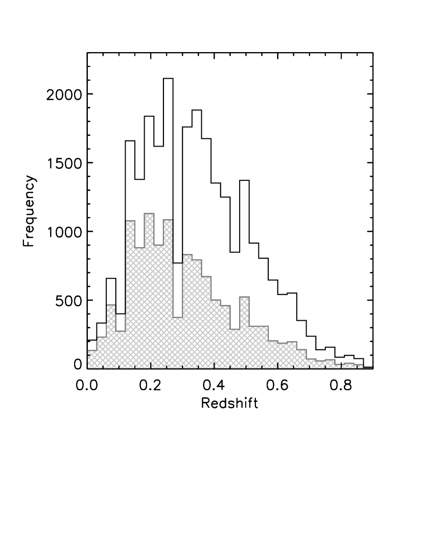
Figure 1.— Redshift histogram of primary sample galaxies from AGES (grey). The unshaded histogram shows the re-weighted sample after the affects of our a priori sparse sampling have been removed from the survey. From this histogram alone, one can see the effects of large-scale structure, even on our 7.6 deg² field.

We give full details of the selection function in Appendix A. In brief, the parent galaxy sample has 26,033 galaxies brighter than $I_{AB}=20.45$. We estimate this photometric sample to be 4% incomplete. AGES observed approximately 50% of this parent sample, 12,473 galaxies. Nearly all of the difference is due to our a priori sparse sampling which can be corrected exactly with our known targeting rates. The sample has a 4.3% incompleteness in assigning fibers to targets and a 2.1% incompleteness in measuring a reliable redshift from an assigned fiber. The Appendix describes our modeling of these incompletenesses, but the main point is that AGES is highly complete and that the error in our incompleteness corrections are smaller than our statistical uncertainties.

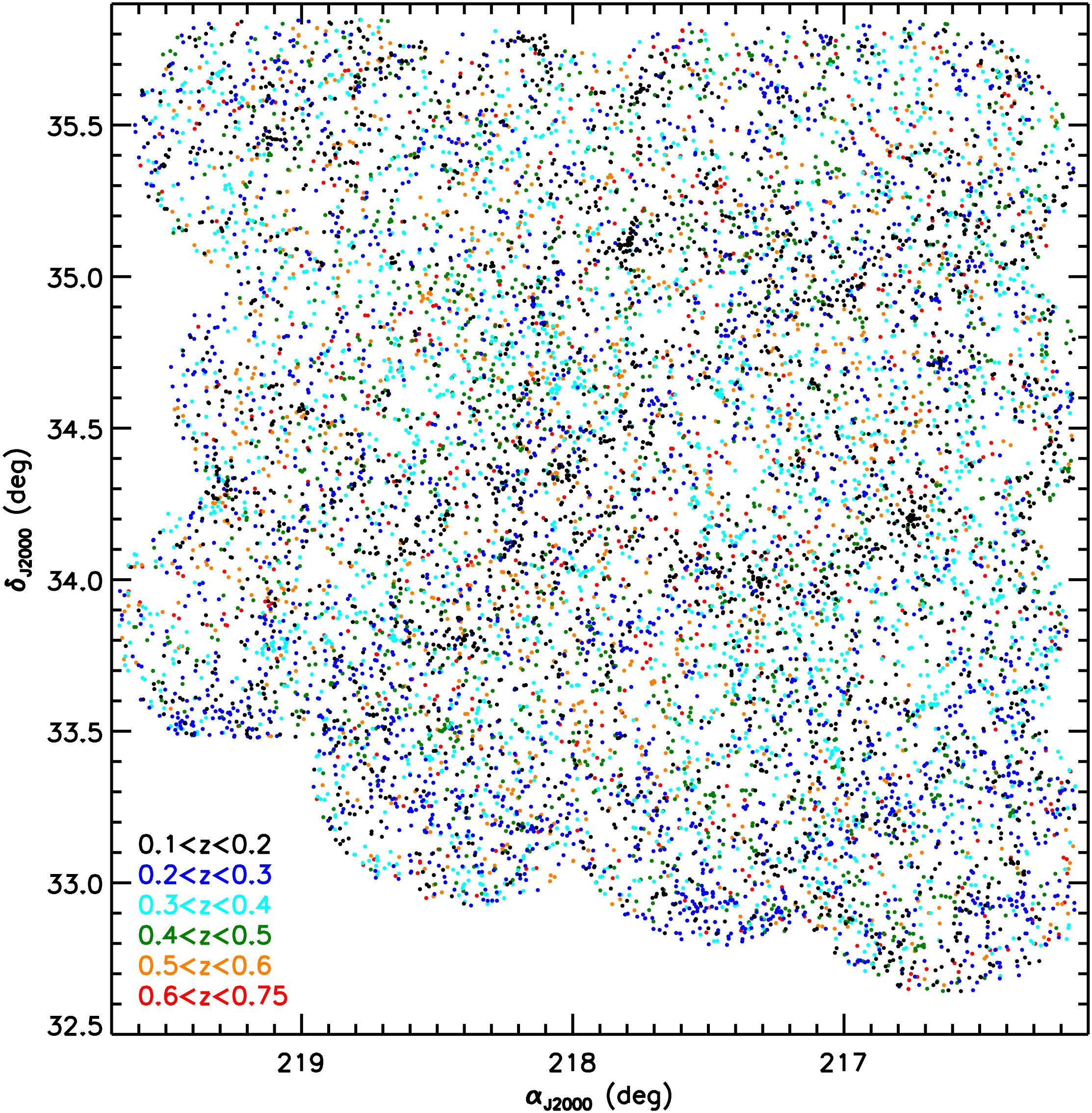
Figure 2.— Angular distribution of AGES spectroscopic galaxies. The points show the spatial distribution of galaxies at $0.1<z<0.75$. At all redshifts, large scale structure is apparent. The circular boundaries are defined by the circular field of view of the Hectospec instrument. While some spectroscopy exists outside this footprint, we only include galaxies in the statistically complete main survey field (AGES fields 1-15) in this figure and in our analysis.

3. Photometry and $K$-Corrections

3.1. $k$-corrections

We construct our luminosity functions from the $I$-band NDWFS photometry using the Sextractor (Bertin & Arnouts, 1996) AUTO (Kron-like (Kron, 1980)) magnitude. The $I$-band photometry is contaminated in certain regions from the low-surface-brightness wings of bright stars which bias the AUTO magnitudes brighter than reality. We address this by constructing a surrogate $I$-band total magnitude, $I_{R}$ from the $R$-band AUTO magnitude plus the $I-R$ color measured in a $6^{\prime\prime}$ aperture (as the aperture colors are much less sensitive to the low surface brightness tails which affects the $R$-band imaging much less than the $I$-band). We then compare $I_{R}$ to the $I$-band AUTO magnitude and compute $I_{\rm tot}$. In the case of two significantly different values between $I$ and $I_{R}$, $I_{\rm tot}$ is the fainter of the two magnitudes. Otherwise, $I_{\rm tot}$ is the average of the two. Explicitly, we compute

$$f=\exp[-(I_{\rm AUTO}-I_{R})^{2}/0.2^{2}]$$ (1)

and use this to linearly combine the average flux of the pair and the smaller flux of the pair

$$I_{\rm tot}=\frac{I_{\rm AUTO}+I_{\rm R}}{2}f+(1-f){\rm max}(I_{\rm AUTO},I_{\rm R}).$$ (2)

About 10% (5%) of the galaxies have a correction of more than 0.1 (0.5) magnitudes. Most of the galaxies have a tight correlation between $I_{\rm tot}$ and $I_{\rm AUTO}$ with an rms of 0.02 mag and $\langle I_{\rm tot}-I_{\rm AUTO}\rangle=0.005$. Because of this slight scatter, we cut our statistical sample of galaxies at $I_{\rm tot}<20.40$; this excludes 2% of the galaxies.

When computing $k$-corrections, we estimate the $B_{W}$, $R$, and $z^{\prime}$ magnitudes by adding $4^{\prime\prime}$ aperture $B_{W}-I$ and $R-I$ and $I-z$ colors to $I_{\rm tot}$. In other words, the SED (colors) of each galaxy is determined by the $4^{\prime\prime}$ aperture colors while the total amplitude is set by the $I_{\rm tot}$ magnitude. We find only 1% shifts in the colors of galaxies when we use PSF-matched images to measure aperture colors. Such shifts do not affect any of our results.

All $k$-corrections are computed using kcorrect v4_2 (Blanton & Roweis, 2007). This procedure uses a linear combination of galaxy spectral templates with the measured photometry and redshifts to construct a best-fit spectral energy distribution (SED) for each galaxy in our sample. These best fitting SEDs are then used to predict the luminosity and colors of each galaxy as a function of redshift. In order to minimize the effects of the $k$-corrections on our final results, we shift to bands that minimize the change in rest-frame wavelength between observed and rest wavelength at a typical AGES redshift. We use the $I$ band to construct the ${}^{0.1}r$ luminosity. Throughout the paper we utilize a ${}^{0.1}ugriz$ filter system. In this system the notation ${}^{0.1}r$ denotes the luminosity in the SDSS $r$ band (Fukugita et al., 1996) shifted blueward by $z=0.1$. This is least sensitive to the SED model at $z=0.42$ where the observed $I$-band matches the rest wavelength of ${}^{0.1}r$ . This choice also makes it easy to compare to the SDSS luminosity function (Blanton et al., 2003). In order to compare our results to those in the literature, we also use the $B_{W}$ band to construct the $B$-band luminosity for each target.

3.2. Red and Blue Galaxies

In order to probe the evolution of red and blue galaxies separately, we first need to select each type of galaxy as a function of redshift in the AGES sample. As galaxies, especially on the red sequence, have undergone substantial passive evolution since $z=1$, a single rest-frame color cut will not lead to a a homogeneous sample of red and blue galaxies over a wide range of redshifts. Here, we solve for the evolution in the red-sequence zeropoint empirically and use that cut when defining red and blue galaxies in the sample. We first construct the luminosity-dependent statistic

$$A=^{0.1}u-^{0.1}r+0.08(M_{{}^{0.1}r}+20).$$ (3)

We then iteratively find the median value of $A$ for galaxies with $A>A_{{\rm med},{n-1}}-0.3$ where $A_{{\rm med},{n-1}}$ is the previous median value; the cutoff value of $A=0.3$ was chosen to best localize the minimum of the galaxy number distribution in color at $z=0.1$. We use only galaxies with $M_{{}^{0.1}r}<-20$ in this procedure. These medians converge to the median color of the red sequence at $M_{{}^{0.1}r}=-20$. We perform these medians in redshift bins of $\Delta z=0.1$ and find values of $A_{{\rm med}}=2.74,2.69,2.64,2.60,2.56,2.52$ for bins centered at redshifts 0.1, 0.2, 0.3, 0.4, 0.5, and 0.65 respectively. We then define our red and blue galaxy samples by linearly interpolating the $A$ parameter to the redshift of each galaxy; galaxies which have $A_{\rm gal}<A_{\rm median}(z)-0.3$ are classified as blue while those redward of that limit are classified as red. Figure 3 shows the ${}^{0.1}(u-r)$ versus $M_{{}^{0.1}r}$ color-magnitude relation in six redshift slices from the AGES sample. The bimodality in galaxy colors is clearly seen in each slice. The color cut used to differentiate between red and blue galaxies in each slice is also shown.

Figure 3.— Restframe ^0.1(u–r) versus $M_{{}^{0.1}r}$ color-magnitude diagram from AGES. The bimodality of galaxy optical colors is apparent in each redshift bin. The dot-dashed line shows the criteria used to separate red and blue galaxies as defined in the text.

3.3. SDSS Comparison Sample

At low redshift, the AGES luminosity function is significantly impacted by large-scale structure and the limited volume we probe. We therefore use the NYU Value-Added Galaxy Catalog (VAGC) to construct a comparison sample of 571,909 galaxies from the SDSS (Blanton et al., 2005) based on the SDSS DR7. From this sample, we extract all galaxies with $0.01<z<0.15$, which we refer to as the SDSS sample.

4. The Galaxy Optical Luminosity Function

Based on the galaxy selection function described in Appendix A, we can reconstruct a statistical sample of $I_{\rm tot}<20.40$ galaxies. We calculate luminosity functions for these galaxies using two methods, the $1/V_{\rm max}$ method and using parametric maximum likelihood models.

4.1. The $1/V_{max}$ Method

The $1/V_{\rm{max}}$ method is one of the more simple and intuitive forms for deriving the luminosity function. The $1/V_{\rm{max}}$ method benefits from being calculated without the need for an a priori parametric form of the luminosity function. In this paper we follow the techniques described in Eales (1993), Lilly et al. (1995), Ellis et al. (1996), Takeuchi et al. (2000), and Willmer et al. (2006). For each galaxy in our sample, we first calculate $z_{\rm{max}}$ and $z_{\rm{min}}$, the full range of redshift for which the galaxy may have been selected through our direct $I_{\rm tot}<20.4$ cut including effects of the $k$-correction and luminosity distance. We then calculate the maximum volume each galaxy could have occupied and been included when considering all galaxies in a given redshift range set by $z_{\rm{lower}}$ and $z_{\rm{upper}}$:

$$V_{\rm{max}}(i)=\int_{\Omega}\int^{z_{\rm{max},i}}_{z_{\rm{min},i}}\frac{d^{2}V}{d\Omega dz}dzd\Omega.$$ (4)

Here, $z$ is the redshift and $\Omega=7.6\,\rm{deg}^{2}$ is the solid angle covered by the survey. The limits of the inner integral are given by

$$z_{\rm{max},i}={\rm min}\{z_{\rm{max}},z_{upper}\}$$ (5)

$$z_{\rm{min},i}={\rm max}\{z_{\rm{min}},z_{lower}\}.$$ (6)

Once we have the $V_{max}$ values for each galaxy in a redshift slice, we can calculate the integral luminosity function in a given magnitude range with $M_{\rm bright}<M<M_{\rm faint}$ using :

$$\phi(M)\Delta M=\sum_{i=1}^{N_{\rm gal}}\frac{w_{i}}{V_{\rm{max}}(i)}.$$ (7)

Here, the $w_{i}$ are the statistical weights described in Appendix A used to correct our sample into a full $I_{\rm tot}<20.4$ flux-limited sample and $\phi$ is the luminosity function. The error for estimates in the $1/V_{\rm{max}}$ method are determined by:

$$\sigma_{\phi}=\sqrt{\sum_{i}\frac{w_{i}}{V_{\rm{max}}(i)^{2}}}$$ (8)

4.2. Parametric Maximum Likelihood Methods

We also use a parametric maximum-likelihood fit to a Schechter function using the STY estimator (Sandage et al., 1979; Efstathiou et al., 1988). We utilize the standard Schechter (1976) function of the form:

$$\phi(L)dL=\phi_{*}(L/L_{*})^{\alpha}e^{-L/L_{*}}dL.$$ (9)

Here, $L_{*}$ characterizes the break in the luminosity function, $\alpha$ sets the faint-end slope, and $\phi_{*}$ is the normalization. Re-writing this in magnitudes we obtain

$$\phi(M)dM=0.4\mbox{ln}(10)\phi_{*}10^{-0.4(M-M_{*})(\alpha+1)}\exp\left(-10^{-0.4(M-M_{*})}\right)dM.$$ (10)

The maximum likelihood method tests the free parameters of the parameterization ($M_{*}$ and $\alpha$ here, but not $\phi_{*}$) by calculating the probability of observing a galaxy with luminosity $M$, given its observed redshift, $z$, and the survey selection function $s(M,z)$. Explicitly, the likelihood for galaxy, $j$, is

$$p(M_{j},z_{j})=\frac{\phi(M_{j})s(M_{j},z_{j})}{\int\phi(M)s(M,z)dM}$$ (11)

where the integral is over the full luminosity range of the survey and the selection function, $s(M,z)$, includes information about the sample flux-limit. The corresponding quantity for the full sample is the product of the likelihood over all galaxies. Finally, we maximize the quantity

$$\mathcal{L}=\sum_{j}{\rm log}\ p(M_{j}|z_{j})$$ (12)

as a function of the $M_{*}$ and $\alpha$ parameters.

Due to the ratio in equation (11), the normalization, $\phi_{*}$ is unconstrained by the STY method. We use the minimum variance estimator of Davis & Huchra (1982) to perform the normalization

$$n=\frac{\sum_{j}f(z_{j})}{\int dV\eta(z)f(z)}$$ (13)

where $n$ is mean number density of galaxies in the sample,

$$f(z)=\frac{w_{i}}{1+nJ_{3}\eta(z)}$$ (14)

is the weight for each galaxy and the selection function is given by

$$\eta(z)=\frac{\int_{max(L_{\rm min}(z),L_{\rm faint})}^{min(L_{\rm max}(z),L_{\rm bright})}dL\phi(L)}{\int_{L_{\rm faint}}^{L_{\rm bright}}\phi(L)dL}.$$ (15)

The luminosity function normalization is given by

$$\phi_{*}=\frac{n}{\int^{M_{\rm faint}}_{M_{\rm bright}}\phi(m)dM}.$$ (16)

The contribution of galaxy clustering to the number density is accounted for using the second moment, $J_{3}=\int_{0}^{r}r^{\prime 2}\xi(r^{\prime})dr^{\prime}$, of the two-point correlation function $\xi(r)$. Since $n$ appears in the weight, $f(z)$, we determine it iteratively using

$$n=\frac{1}{V}\sum_{j}\frac{1}{\eta(z_{j})}$$ (17)

as our initial guess. Finally, when calculating the luminosity density, we integrate the best-fitting luminosity function

$$j(z)=\int L\phi(L)dL=L^{*}\phi^{*}\Gamma(\alpha+2)$$ (18)

where $M_{\odot,r^{0.1}}=4.76,M_{\odot,B}=5.48$, and $\Gamma$ is the Gamma function. This form of integration to measure the luminosity density does not depend on the limiting magnitude of the survey but does depend on the form of the luminosity function in order to extrapolate to the entire population. Since the majority of the luminosity is located at $M^{*}$ for a population following a Schechter function, only the highest redshift bins in this survey extrapolate more than 50% of the luminosity density when calculating the total $j$ compared to the luminosity range probed by the survey; at the lowest redshifts considered, we probe 80-95% of the total galaxy luminosity density.

4.3. Luminosity Function Results

Figure 4 shows the resulting optical luminosity functions in the ${}^{0.1}r$ band for SDSS galaxies at $0.01<z<0.15$. The points are the 1/$V_{\rm max}$ result and the lines are the best fitting STY luminosity functions. We used this SDSS luminosity function to fit the value of the Schechter $\alpha$ parameter when fitting the AGES data, as the AGES luminosity function in the lowest redshift bin are limited by the small volume probed. We restrict our fitting of the SDSS data to galaxies between $-23<M_{{}^{0.1}r}<-18$. This range was chosen to mirror the luminosities probed by our AGES galaxy sample. In order to test the effects on this range, we also fit the SDSS data with faint limits to $M_{{}^{0.1}r}<-17$ and $M_{{}^{0.1}r}<-17.5$; the range used in the fitting has no strong effect on the derived $\alpha$ parameters. Using STY determined luminosity function parameters (shown as lines in Figure 4), we find $\alpha=-1.05\pm 0.01$ for the full galaxy sample, $\alpha=-1.15\pm 0.02$ for the blue galaxy sample, and $\alpha=-0.50\pm 0.02$ for the red galaxy sample. Throughout the rest of our discussion, we hold these $\alpha$ values fixed for each survey when fitting the AGES data. For comparison, the lowest redshift bin in AGES yields values of $\alpha=-1.06\pm 0.03$ for all galaxies, $\alpha=-0.46\pm 0.09$ for red galaxies, and $\alpha=-1.15\pm 0.04$ for blue galaxies which is in excellent agreement with the SDSS values but with larger uncertainties. In order to test the overall normalization of our luminosity function measurements, we calculate the number counts as predicted from the final derived parameters and compare these to the AGES target number density. We predict $3310.1\pm 118$, $1403.1\pm 80.1$, $1850.1\pm 118$ galaxies per square degree for all, red, and blue galaxies respectively for galaxies with $I<20.4$ and $0.05<z<0.75$; the error term is dominated by the range of $k$-corrections associated with each population. The AGES number counts for galaxies in this magnitude and redshift range are 3269.61, 1420.8, and 1875.13 for all, red, and blue galaxies.

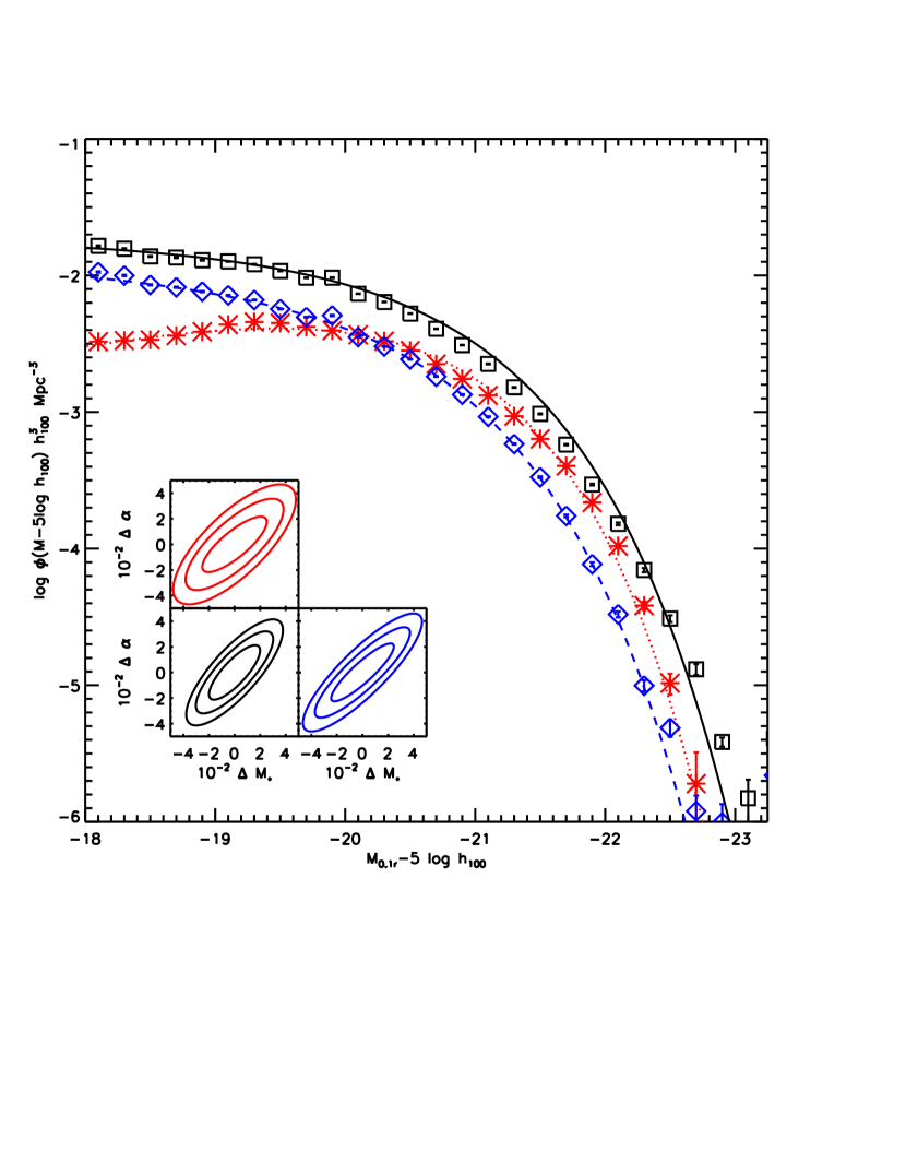
Figure 4.— SDSS galaxy sample ${}^{0.1}r$ luminosity functions for all (black squares), blue (blue diamonds), and red (red asterisks) galaxies as defined in the text. As AGES is limited by large-scale structure in the field at the lowest redshifts, we use these SDSS luminosity functions as an anchor for the evolution we measure based on AGES luminosity functions at higher redshifts. Furthermore, we fit the full shape of the SDSS luminosity functions using the maximum likelihood technique (fits shown with dot-dashed lines) to fit the faint-end slope, $\alpha$, of the galaxy optical luminosity function at $z=0.1$. Since our AGES luminosity functions do not extend significantly fainter than $L_{*}$ at $z>0.3$, we fix the $\alpha$ values used when fitting AGES LFs to those determined from SDSS. Note that these agree with the estimates from the lowest redshift AGES bin but have smaller uncertainties. The inset illustrates the covariance associated with the $M_{*}$ and $\alpha$ measurements based on these luminosity functions.

Figure 5.— Same as Figure 4 but showing the B-band luminosity function for SDSS galaxies at $z=0.1$. Again, we fit the SDSS luminosity functions to determine the local $\alpha$ value in the $B$-band and then assume $\alpha$ is fixed in redshift.

As the luminosity function has historically been measured in the $B$-band, we also $k$-correct the SDSS galaxy photometry to the restframe ($z=0$) $B$-band and measure the galaxy $B$-band luminosity function from SDSS for comparison. Figure 5 shows the $B$-band luminosity functions for SDSS galaxies at $0.01<z<0.15$. Again, we use the $\alpha$ values derived from these low-redshift fits to fix the values used when fitting AGES luminosity functions at higher redshift. In the $B$-band we find that $\alpha=-0.99\pm 0.02$ for the full SDSS sample, $\alpha=-1.10\pm 0.03$ for blue galaxies and $\alpha=-0.45\pm 0.02$ for red galaxies.

We show the ${}^{0.1}r$-band AGES galaxy optical luminosity functions based on the $1/V_{max}$ method in Figures 6-8 and list our $1/V_{\rm max}$ measurements in Tables 1-3. In each figure, the grey line shows the $z=0.1$ luminosity function of all SDSS galaxies. The data points show the $1/V_{\rm max}$ luminosity function measurements and the solid dashed lines show the STY determined parameterization. As an added check on our luminosity function calculation, we further plot the summed red galaxy and blue galaxy luminosity functions to compare the with total galaxy luminosity function in Figure 6; the summed luminosity function agrees well with the total galaxy luminosity function. The typical luminosity of galaxies increases with redshift. That is, the stellar populations of galaxies of all colors has, on average, faded from $z=0.75$. The best fitting parameters determined from our STY fits are listed in Table 4.

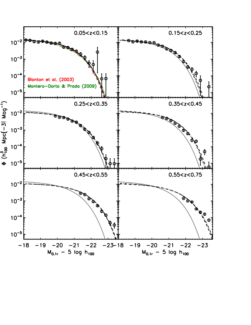
Figure 6.— AGES ${}^{0.1}r$ luminosity function for all galaxies at $0.05<z<0.75$. Each panel shows the optical luminosity function in bins of increasing redshift with the redshift range listed in the upper right corner of the panel. The dashed line shows the best fitting STY parameterization while the data points with error bars show the $1/V_{\rm max}$ measurements. The data points show the $1/V_{max}$ method determination of the luminosity function and the grey line shows the SDSS $z=0.1$ LF for all galaxies. Evolution is clearly detected; galaxies in the past were, on average, more luminous than they are at the present epoch. The dot-dashed lines show the sum of the blue and red galaxy luminosity functions shown in Figures 7 and 8. The total luminosity density from AGES agrees well with the total of the red and blue populations. Additionally, we plot the $z=0.1$ SDSS luminosity functions from Blanton et al. (2003) and Montero-Dorta & Prada (2009) for comparison.

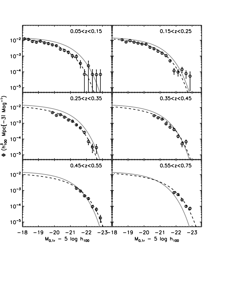
Figure 7.— Same as Figure 6, but only including blue galaxies as defined by the empirical red/blue classification described in the text and shown in Figure 3. For reference, the $z=0.1$ LF for all galaxies determined from SDSS data is shown in grey.

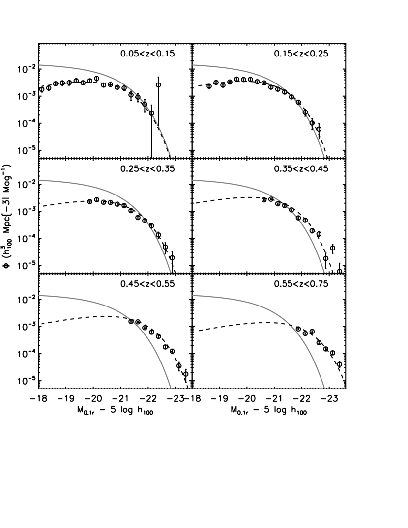
Figure 8.— Same as Figures 6 and 7, but now for red galaxies. Again, the grey line shows the LF for all galaxies at $z=0.1$ from SDSS.

We estimate uncertainties for our fitted parameters using a two-part strategy. First, to include the effects of small-scale structure and shot noise, we use a jackknife method. We split the sample into 15 roughly equal-area subregions on the sky (the 15 AGES fields) and repeat our fits excluding one area at a time. The rms variation between N such samples, multiplied by $\sqrt{N-1}$, is an estimate of the uncertainty in each parameter. In this test, we calculate the luminosity density for each subsample before the variance is computed in order to account for the covariance between $M_{*}$ and $\alpha$.

These jackknife error estimates would be correct if the subregions were statistically independent from each other. However, it does not account for the correlations between subregions due to large-scale structure, most notably on scales larger than the survey region as a whole. This large-scale structure contribution can be calculated from the two-point correlation function. We compute the large-scale structure contribution by averaging the correlation function across all pairs in a given redshift shell within our survey volume. This gives the variance of the fractional over density in the survey region. As the AGES survey is reasonably large, we use the linear-regime power spectrum from the WMAP-3 cosmology (Spergel et al., 2007) to generate the correlation function. The averaging over pairs is accelerated by projecting the partial correlation function to the angular correction function using the Limber approximation and then performing a Monte Carlo angular integration using a set of points randomly distributed in the survey area. The results differ only modestly from the rms density fluctuations in a sphere whose volume equals that of the survey in the given redshift bin.

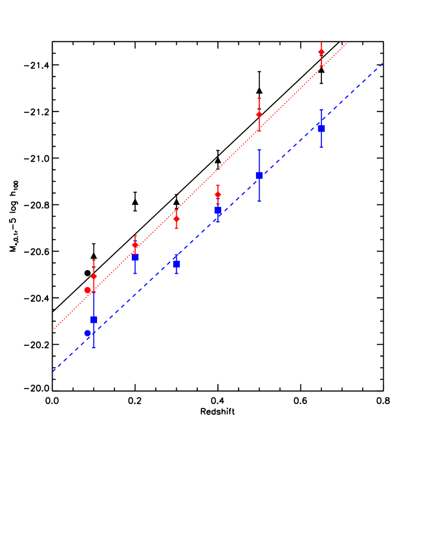
Figure 9.— Best fitting $M_{*}$ in the ${}^{0.1}r$ band based on STY fits to the AGES lgalaxy sample. The empty symbols show the AGES data for all galaxies (black triangles), red galaxies (red diamonds), and blue galaxies (blue squares). The filled circles show the best fitting SDSS values (the SDSS measurement is at $z=0.1$, but has been shifted to slightly lower redshift for plotting clarity). All galaxies in the survey evolve similarly although the red galaxies fade slightly faster with redshift than the full galaxy sample or blue galaxies. We find that $M_{*}$ for the full sample fades by $1.67\pm 0.07$ mag per unit redshift, the blue sample fades by $1.66\pm 0.09$ mag per unit redshift while the red galaxies fade by $1.73\pm 0.07$ mag per unit redshift. The lines show the best fitting evolution for all (solid), red (dotted), and blue (dashed) galaxies.

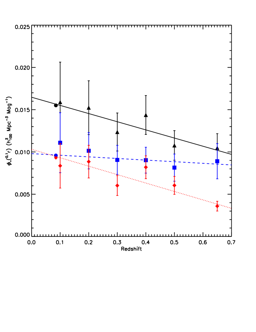
Figure 10.— Best fitting $\phi_{*}$ values in the ${}^{0.1}r$ band determined from our STY analysis. As in Figure 9, the full galaxy sample is plotted with black triangles, the red galaxies with red diamonds, and the blue galaxies with blue squares. The best fitting evolution is shown with solid, dotted, and dashed lines, respectively. We find that the number density of all galaxies has increased since $z\sim 0.7$ with the red galaxies showing the most dramatic increase in number density. The fits are constrained to go through the SDSS measurement at $z=0.1$ (filled circles), as the lowest-redshift bin from AGES is highly susceptible to large scale structure due to its relatively small area of the survey. When fitting the data, we use a model of the form $\phi_{*}\propto 1+Pz$. We find that the trend in the full population ($P=-0.59\pm 0.14$) is driven primarily by a sharp decline in the red population ($P=-0.95\pm 0.10$) while the blue galaxies show much less evolution ($P=-0.38\pm 0.21$).

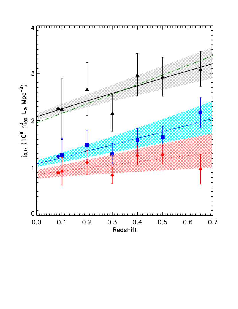
Figure 11.— Evolution of the ${}^{0.1}r$ luminosity density for all (black triangles), blue (blue squares), and red (red diamonds) galaxies from AGES. The SDSS measurement at $z=0.1$ is shown by the filled circles which have been slightly offset in redshift for clarity. We model the evolution as $j\propto(1+z)^{n}$; the best fitting models are also plotted as the solid, dotted, and dashed lines for the full, red, and blue samples respectively. We find that the full sample evolves with $n=0.81\pm 0.27$, the blue galaxies with $n=1.64\pm 0.39$, and red galaxies with $n=0.54\pm 0.64$. While the number density of red galaxies has increased since $z=0.7$, the luminosity density in red galaxies grows much more slowly over that time. For comparison, the green dot-dot-dot-dashed line shows the sum of the best fitting trends for the red and blue galaxies; the sum of each population separately agrees well with the total population within experimental errors.

In detail, the variance of the density field of the full region is not independent of the variance reported by the jackknife method. This is unavoidable; while modes much larger than the survey are invisible to the jackknife method, a single large cluster would affect the jackknife errors as well as the overall density variation. We remove this double counting by using the Monto Carlo integration to estimate the covariance matrix between the 15 sub-regions and predicting the jackknife variations in linear theory.

If we have $N$ regions on the sky, with areas $A_{j}$ and a total area of $A$, then the covariance between the overdensities, $C_{ij}$of two of the regions is

$$C_{ij}=\int_{\vec{\theta}_{i}\in A_{i}}{d\vec{\theta}_{i}\over A_{i}}\int_{\vec{\theta}_{j}\in A_{j}}{d\vec{\theta}_{j}\over A_{j}}w(|\vec{\theta}_{i}-\vec{\theta}_{j}|)$$ (19)

where $w(\theta)$ is the angular correlation function. Constructing a Monte Carlo set of random points in the union of these regions, with $N_{i}$ points in region $i$, the integral can be computed as

$$C_{ij}={1\over N_{i}N_{j}}\sum_{pq}w(|\vec{\theta}_{p}-\vec{\theta}_{q}|)$$ (20)

where the sum is over points $p$ in region $i$ and points $q$ in region $j$. The covariance of the overdensity of the full region is

$$\sigma_{total}^{2}=\sum_{ij}A_{i}C_{ij}A_{j}/A^{2}$$ (21)

which is the same as if one had integrated the angular correlation function of pairs of points in the full region. The variance from jackknife is approximately $\sum_{j}C_{jj}/N^{2}$; this assumes that the regions are equal in area so as to simplify the formula considerably (i.e. it assumes that the densities from the $N$ regions are being combined with equal weight rather than weighting by area). This assumption is true to within 12% rms for the 15 AGES regions used in our calculations.

Typically, the jackknife variance is about 25% of the total variance. We then subtract this jackknife variance from the full density-field variance to yield the variance $\sigma_{LSS}^{2}$ resulting from structure larger than the survey volume. Our estimate of the fractional variance in the luminosity density will be the sum of this variance and the variance from the actual jackknife estimation. By subtracting off the linear theory jackknife prediction and adding back the actual jackknife error, we include the non-linear aspects of the correlation function and the shot noise to our error estimate. As the AGES galaxies are not strongly biased relative to the dark matter (Hickox et al., 2009), we expect this estimate to be a robust measurement of the variance from large scale structure.

For our six redshift slices, we find $\sigma_{LSS}/j$ of 0.277, 0.203, 0.168, 0.144, 0.1128, and 0.079 (from low to high redshift) assuming a linear theory normalization of $\sigma_{8}=1.0$ for galaxies. In all but the highest redshift bin, this error is larger than the 5-10% jackknife variance estimate in the luminosity density. Hence, the uncertainty in the estimate of the luminosity density in AGES is dominated by large-scale structure.

Figures 9-11 show the redshift dependence of $M_{*}$, $\phi_{*}$, and the luminosity density $j$ for each of the three galaxy samples in the ${}^{0.1}r$ band. Evolution is clearly detected. In all three samples, $M_{*}$ is brighter in the past. The slope of this evolution is roughly 1.6 in all three cases. We also find a drop in $\phi_{*}$ toward higher redshifts, predominately for the red galaxies. For the red galaxies, the rise in $M_{*}$ balances the drop in $\phi_{*}$ so the luminosity density of red galaxies is roughly constant. For blue galaxies, the rising $M_{*}$ dominates and the luminosity density increases by 60% from $z=0.1$ to $z=0.6$. The luminosity density of all galaxies increases by 50% over the same epoch.

Table 5 lists the best fitting evolution of $M_{*}$, $\phi_{*}$, and $j_{{}^{0.1}r}$ for the AGES sample. We assume functional forms such that $M_{*}(z)=M_{*}(0)+Qz$, $\phi_{*}\propto 1+Pz$, and $j_{{}^{0.1}r}\propto(1+z)^{n}$. The table lists the best fitting values for $Q$, $P$, and $n$ for each galaxy population. In each of these fits, we perform a $\chi^{2}$ fit of each form to the measured parameters and associated errors and solve for the best fitting $Q$, $P$, and $n$ value. While we opt to fit the parameters derived in each redshift bin, more sophisticated techniques exist allow one to fit the full galaxy population across all redshifts while simultaneously fitting for the evolutationary parameters (Lin et al., 1999; Heyl et al., 1997).

4.4. Comparison with Previous Work

As the majority of work on the galaxy optical luminosity function has focused on the restframe $B$-band, we also measure the evolution of the AGES LF in that band. When constructing the $B$-band luminosity function, the observed $R$-band is a close match to the effective wavelength of the rest-frame $B$-band across the redshift range probed by AGES (with the closest comparison at $z\sim 0.5$). In order to properly construct the likelihood when constructing this sample, we implement an effective $R$-band magnitude cut on the sample to ensure that the $I$-band AGES selection does not bias our sample toward red galaxies. This effective cut, however, has little impact on our sample and results in the removal $<0.5\%$ of our sample galaxies when constructing the $B$-band luminosity function. We use the SDSS values for $\alpha$ at $z=0.1$ derived from the luminosity functions in Figure 5 and assume the AGES $B$-band luminosity functions have fixed faint-end slopes relative to the SDSS value. Figures 12-14 show the AGES $B$-band luminosity functions compared with luminosity functions from the literature for all galaxies, blue galaxies, and red galaxies respectively. The $1/V_{\mbox{max}}$ luminosity function measurements are presented in Tables 6-8. The best fitting STY parameters for the $B$-band luminosity functions are listed in Table 9.

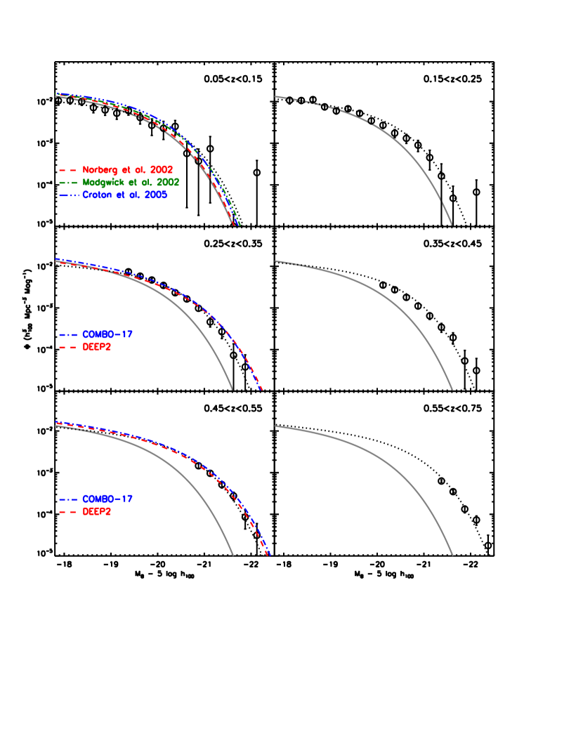
Figure 12.— AGES $B$-band total galaxy luminosity function. In each panel, the data points and errorbars show the $1/V_{max}$ derived luminosity functions, the grey line shows the SDSS total galaxy luminosity function and the dotted line shows the sum of the AGES blue and red galaxy luminosity function. For comparison, we have also plotted best fitting luminosity functions from Norberg et al. (2002), Madgwick et al. (2002), and Croton et al. (2005) from 2dF at low redshift and from DEEP2 and COMBO-17.

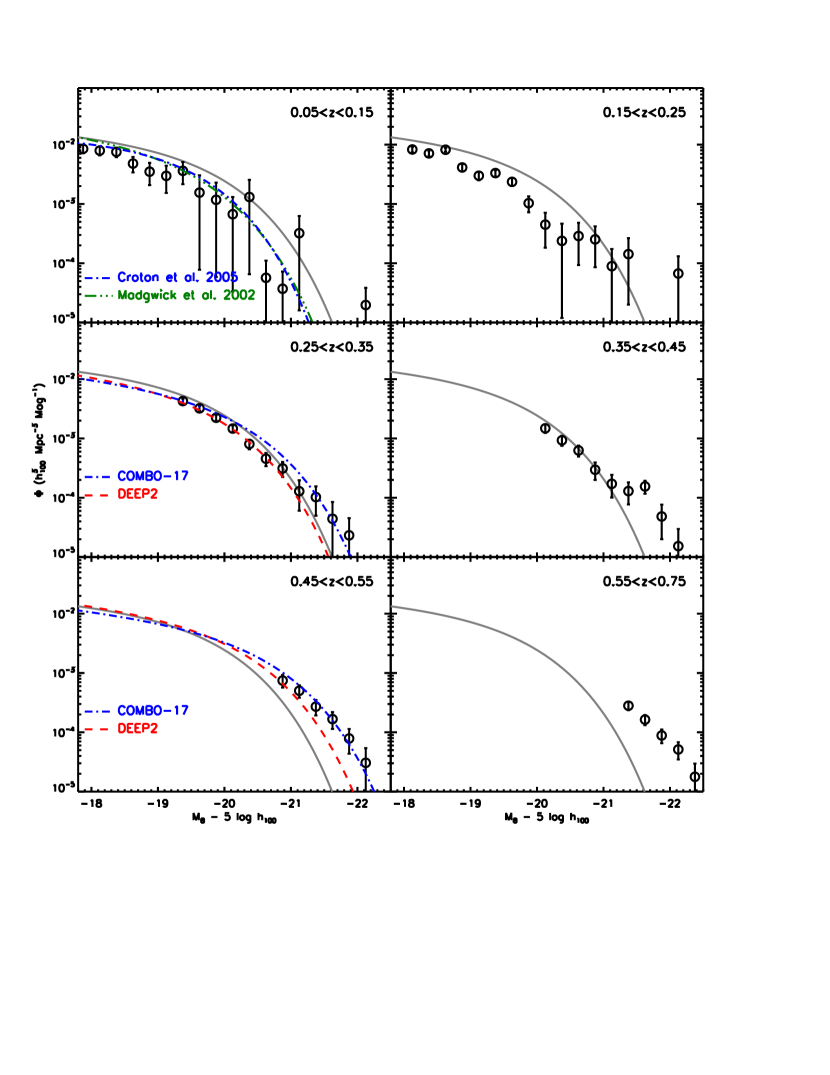
Figure 13.— Same as 12 but showing the blue galaxy $B$-band luminosity function from AGES.

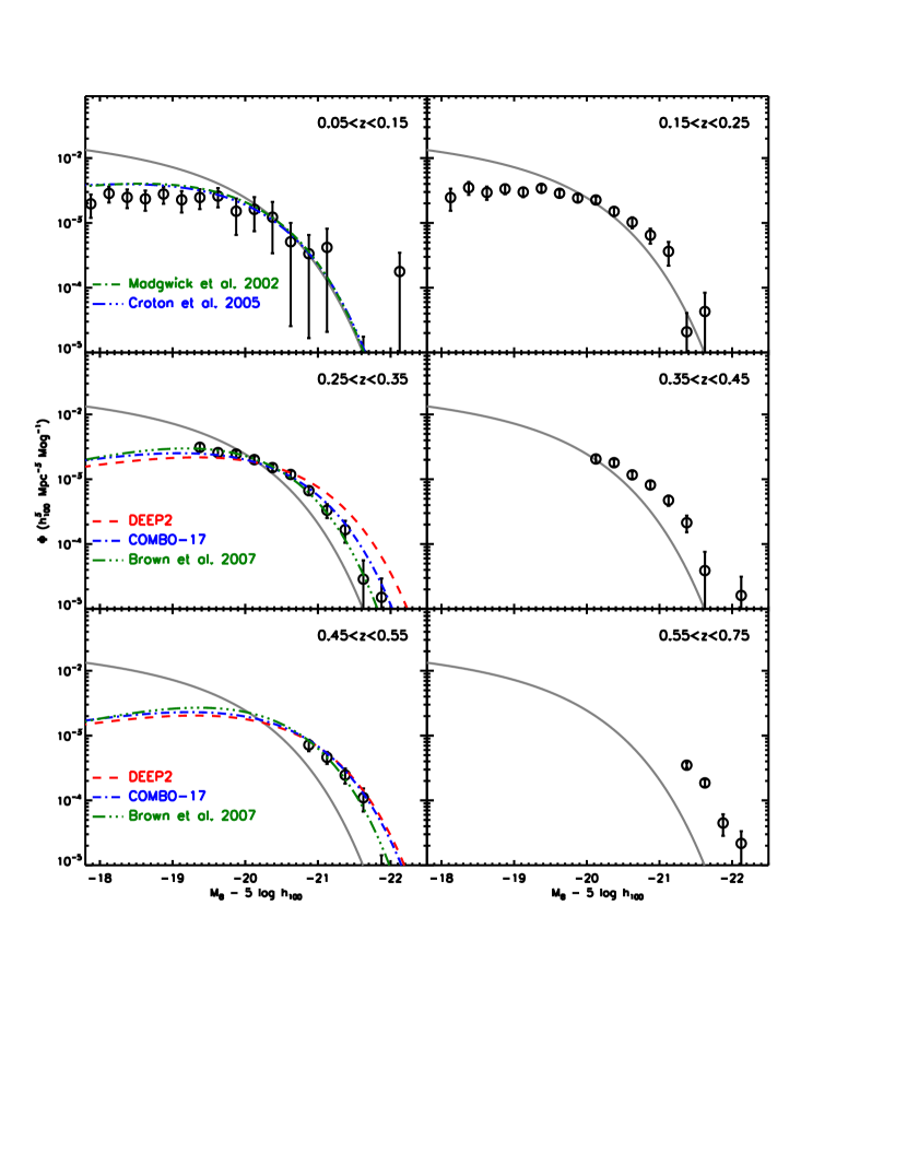
Figure 14.— Same as 12 but showing the red galaxy $B$-band luminosity function from AGES.

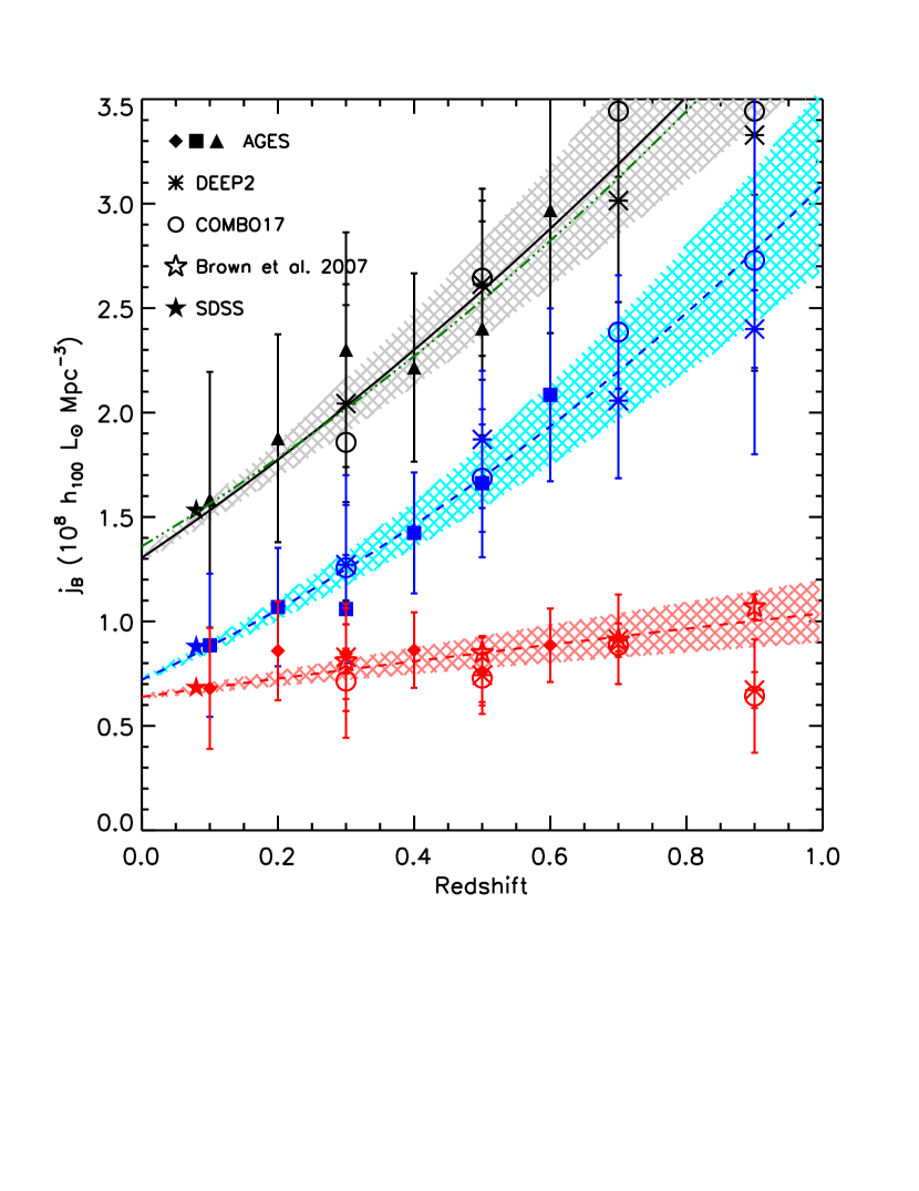
Figure 15.— The evolution of the $B$-band luminosity density from AGES and the literature. The AGES luminosity density measurements for all galaxies (solid black triangles), blue galaxies (solid blue squares), and red galaxies (solid red diamonds) is fit using the $z=0.1$ SDSS measurements (filled circles) as a required constraint. We also show the measurements from DEEP2 (asterisks) and COMBO17 (empty circles) for each of the galaxy populations. Finally, we also show the estimates of Brown et al. (2007) for red galaxies with stars. For illustration, we extrapolate our fits at low redshift to $z=1$ and show the $1-\sigma$ confidence as the grey, cyan, and pink shaped regions. Overall, the extrapolations of our fits at low-redshift agree well with the measurements in the literature at higher redshift. While current surveys either probe the low-redshift or high-redshift end of this distribution, with little existing data able to span the entire range and allow for detailed measurements within a single survey, overall the results from high- and low- redshift seem to agree. As in Figure 11, the green dot-dot-dot-dashed line marks the sum of the best-fitting red and blue luminosity densities.

Figure 15 shows the AGES measured B-band luminosity density, $j_{B}$, for all, red, and blue galaxies as well as measurements for each sample from DEEP2 (Faber et al., 2007) and COMBO17 (Wolf et al., 2003). We also include the luminosity density measurements of Brown et al. (2007) which include red galaxies with photometric redshifts also drawn from the NDWFS field. As the Brown et al. (2007) sample covers the same area based on the same photometric data, it shares the same photometric systematics and large scale structure systematics as our AGES data. The dot-dashed lines and shaded areas show the best fit evolutionary tracks for each type of galaxy fit using only the SDSS and AGES data. The shaded regions show the $1\sigma$ confidence regions based on the AGES and SDSS extrapolated to $z=1$.

Overall, the extrapolations of the AGES evolution agrees with the measurements made in the literature and often lie between the measurements from DEEP2 and COMBO-17. It it worth noting that if our extrapolation is extended to $z=1$, the DEEP2 red galaxy luminosity density is quite low while the Brown et al. (2007) measurement is slightly above our prediction. Clearly the ideal manner of studying the full evolution from $z=1$ to today, however, is a large deep survey of spectroscopically observed galaxies with the area and depth to probe the full $z<1$ epoch with robust statistics.

5. Conclusions

We have computed the optical luminosity function from the AGN and Galaxy Evolution Survey sample. This is the largest spectroscopic sample currently available of field galaxies at $0.3<z<0.7$. At low redshifts, the luminosity function from AGES is in excellent agreement with the much larger SDSS dataset. At higher redshift, we see clear evidence for evolution of the luminosity function, with $M_{*}$ being brighter at higher redshift. We compute the evolution of the luminosity density for the full sample as well as for the populations of blue and red galaxies separately. We find that the evolution of the luminosity density of red galaxies over the $0.1<z<0.65$ is nearly constant in the ${}^{0.1}r$ band, $(1+z)^{0.54\pm 0.64}$, while that of blue galaxies evolves rapidly, $(1+z)^{1.64\pm 0.39}$. Both blue and red galaxies have a similar evolution in $M_{*}$, 1.6 magnitudes per unit redshift at fixed $\alpha$. The amplitude of the luminosity function, $\phi_{*}$, decreases with redshift in all cases, but more so for red galaxies.

The major caveat in these results, aside form the ever-present desire to probe more survey volume, is that our higher redshift samples include only fairly luminous galaxies. Given the observed evolution, the AGES flux limit reaches $L_{*}$ at about $z\sim 0.53$. Hence, our fits are driven by galaxies near or above $L_{*}$. Any inferences about luminosity densities depend on the extrapolation to lower luminosity galaxies via a constant $\alpha$. More data from the next generation of deep spectroscopic surveys which probe larger volumes and constrain fainter galaxies will allow even tighter constraints of the evolution of galaxies over the last half of cosmic history.

Appendix A The AGES Selection Completeness Function

A.1. AGES Galaxy Target Selection

In this section, we outline the galaxy target selection process employed by AGES. AGES also targeted quasars, but we will not describe that selection, here; full details on the AGES execution and target selection can be found in Kochanek et al. (2011) and Assef et al. (2010).

We targeted based on the NDWFS DR3 imaging catalogs. For each band of NDWFS imaging, we define acceptable photometry (bgood, rgood, and igood) the Sextractor flag $\texttt{FLAG}<8$ (i.e. unsaturated, not falling off a chip boundary, or heavily blended), not flagged as a duplicate object, and which had photometric data available ($\texttt{FLAG\_PHOT}=0$). All targets were required to have igood  and at least one of rgood or bgood. Objects were classified as point sources if the stellarity index (Sextractor’s CLASS_STAR parameter) in at least one of the bands had $\texttt{CLASS\_STAR}\geq 0.8$. Galaxy targets are required to be extended by this criterion. All flags discussed here use the default definition provided by Sextractor.

Galaxy targets were restricted to lie in the $15.45<I\leq 20.45$ magnitude range. To avoid the problem of Kron-like (AUTO) magnitudes being corrupted by the halos of nearby stars, we impose limits on the aperture magnitudes of selected objects. If either of the $1\farcs 0$ or $6\farcs 0$ aperture magnitudes were extremely faint, $I_{1\farcs 0}>24.45$ or $I_{6\farcs 0}>21.45$, we removed the galaxy from the sample. These restrictions remove much of the low-surface brightness spurious objects, but not completely. In order to correct for these low-surface brightness contaminants, we first flag objects which are observed near bright USNO stars. For each USNO star in the NDWFS field, we define a scale length

$$\theta_{\rm USNO}=20.0^{\prime\prime}+5.0^{\prime\prime}(15.45-R_{\rm USNO}).$$ (A1)

If the closest USNO star is less than $\theta_{\rm USNO}$ from a galaxy then the galaxy was flagged as being too close to the bright star. If the $6^{\prime\prime}$ galaxy aperture magnitude satisfied

$$I_{6^{\prime\prime}}>I_{tot}+4[(I_{tot}-20.45)/8]^{2}$$ (A2)

the galaxy was rejected. Secondly, if the galaxy was less than $0.5\theta_{\rm USNO}$ from the closest USNO star, the galaxy was removed from the survey. After these cuts, we have a cleaned sample of possible galaxy targets. Table 10 lists the bright sample magnitude range, faint sample magnitude range, and faint sample sampling rate for each of the samples defined for AGES spectroscopy and Table 11 lists the number of targets, number of redshifts obtained, and overall completeness for each AGES galaxy sample. It’s important to reiterate that all of these are cuts in addition to the $I<20.45$ cut; in essence, a galaxy that was a bright detection from our multiwavelength imaging was given higher preference for spectroscopy than galaxies undetected in these other bands.

A.2. Completeness Corrections

We decompose the selection function into 4 terms. First, objects may not have passed target selection cuts due to quirks of the photometry or some aspect of the targeting (“photometric incompleteness”). Second, objects that would otherwise have been selected may have been dropped from our statistical sample due to a priori sparse sampling. Third, a high-priority object may have failed to have a fiber allocated (“fiber incompleteness”). Finally a spectrum may have failed to yield a useful redshift (“redshift incompleteness”).

The AGES galaxy target selection sets flux limits in 12 bands of photometry. However, this complex set of targeting criteria can be thought of as a simple $I<20.45$ sample in which a priori sparse sampling has been done to de-emphasize “common” objects while more heavily sampling the tails of the multicolor distribution. It is easy to undo the sparse sampling and restore a fair $I<20.45$ sample as all of the targeting weights are known exactly. We do not use objects that were rejected by sparse sampling in our analysis though some of these objects did get a spectrum as a “filler” object. We construct the main statistical galaxy sample as the objects with high priority target flags, with all three optical bands present (rgood, igood, and bgood) to ensure good $k$-corrections, and inside the primary galaxy survey region.

About 1.5% of objects fail either rgood  or bgood. There is little coherent structure to these, so it is not a problem of non-overlapping photometry. However, these objects also have a 25% redshift failure rate, which is quite high compared to the full sample. It is likely these objects are corrupt; we estimate that the requirements of 3 bands of good photometry is likely only causing a 1% photometric incompleteness. Furthermore, we rejected galaxies from AGES if they were too close to a bright star; this affects about 2% of the survey region. There are 762 SDSS MAIN sample targets ($r<17.77$) inside the primary survey region. 733 (96%) of these are in the AGES parent sample and 709 (93%) end up being selected. The 3% loss is due to the effects described above. However, the first 4% is yet unaccounted for. Of course, the SDSS has a small rate of spurious targets, about 1%. We therefore conclude that at $r<17.77$, we have an additional 3% incompleteness that we have not identified. This could well improve as one moves to the fainter objects that NDWFS was designed for. In order to ensure that this 3% incompleteness is appropriate for the full galaxy sample and not simply the bright end of the galaxy luminosity function which overlaps with the SDSS MAIN sample, we constructed fake galaxies with sizes and fluxes representative of the AGES galaxy sample and included them in the NDWFS imaging. Reperforming a SEXTRACTOR analysis of the imaging, we find that approximately 3.5% of the galaxies added to the images are unrecovered - typically due to deblending with bright foreground galaxies or stars. This incompleteness value does not strongly depend on the brightness of the galaxy within the range of galaxy fluxes considered for our luminosity function analysis. Brown et al. (2007) found the NDWFS imaging dataset to be more than 85% complete for galaxies of typical sizes and shapes to $I_{AB}=23.7$, several magnitudes deeper than we target with AGES. As the optical imaging used to select AGES target galaxies extends several magnitudes deeper than the flux limit of AGES spectroscopy, we expect little incompleteness to arise from photometric depth at the faint end of our targeting range.

In sum, we believe that the photometric incompleteness is 3-6% (but at the very bright end, e.g. $I<15$, there is surely more incompleteness). The primary galaxy survey region is 7.90 deg² We adopt a 4% catalog incompleteness and adjust the fiducial area to 7.60 deg². The large-scale structure corrections remain tied to the larger area because the incompleteness is in many small disjoint regions.

In order to test the effects of star-galaxy separation on our target selection, we first compare the stellarity classifications between NDWFS and SDSS imaging. We restrict this comparison to bright SDSS objects with robust stellarity measurements; as the depth of NDWFS is considerably deeper than SDSS, extending to the detection limit of SDSS leads to identifying problems with the SDSS star-galaxy separation at faint fluxes rather than to understand the role of NDWFS star-galaxy separation on our luminosity function measurements. The NDWFS photometry reproduce the stellarity measurements from SDSS in this regime. In order to quantitatively test how the separation of stars galaxies effects fainter NDWFS targets, we select all objects with IRAC colors consistent with arising from galaxies (and inconsistent with being either stars or AGNs). We find that $<0.3\%$ of these objects were classified as stars based on their NDWFS stellarity measurements and conclude that our samples do not suffer significant incompleteness due to galaxies becoming poorly resolved in the NDWFS imaging.

Only 1% of the AGES main-sample galaxies lack counterparts in SDSS imaging. Nearly all of these are low surface brightness objects that are plausibly below the SDSS detection limit. Thus, we can limit the rate of spurious objects in the AGES sample to below 1%. In 2005, AGES targeted nearly 300 bright objects, typically $r<17$, that SDSS declared as stars (which is confirmed by AGES spectroscopy). These objects saturated the NDWFS imaging and were mistakenly classified as extended by the star-galaxy separation. To remedy this, we remove all objects at $r<19$ that SDSS called a point source. NDWFS and SDSS agree very well on extended sources between $r=17$ and $r=20$. SDSS obtained redshifts for 27 galaxies included in the AGES primary sample that we didn’t observe at the MMT. We consider these galaxies as having good redshifts when computing fiber and redshift incompleteness.

AGES performs very well as regards to fiber completeness; most regions of the survey were observed at least six times, so even high multiplet groupings could be resolved. In total, 95.7% of targets were observed. Fields 13-15, however, were not as well sampled in 2005. Field 14 is the worst with only 83% completeness. Fields 1-12 have fiber completeness of 98.3%. The level of fiber incompleteness depends on the local environment of the galaxy, as fiber collisions are a major source of the problem (though not the only source). To address this, we seek to assess completeness as a function of local density and number of opportunities for each object to be observed. We first split the objects into those that were high-priority targets in 2004 and those that were not. The 2004 targets have a much higher completeness and are thus treated separately from objects observed in 2005 and 2006. For each object, we count the number of high-priority targets within $30^{\prime\prime}$. For the 2004 targets, we divide them into sets according to the neighbor count and define the fiber completeness as the fraction of objects in each bin that received a fiber. For the 2005 targets, we repeat this but restrict the count to high-priority targets that ere not observed in 2004. We also separate the binning into objects that fell within the field of $<4$, 4, 5, or $>5$ observations in 2005 and 2006. In other words, the fiber completeness of 2005 targets is judged in sets defined by the number of 2005 nights and the number of 2005 and 2006 opportunities. In the extremes of the distribution, a bin can have zero observed galaxies and yet not be empty from non-observed galaxies, which would result in an infinite weight. In these cases, we add objects to the next bin until we have a galaxy that can be up-weighted to compensate for the missing ones. Figure 16 shows the distribution of the final fiber completeness correction derived here as a function of target total magnitude and Figure 17 shows the mean fraction of possible AGES targets that received a valid redshift as a function of the number of nearby neighbor galaxies.

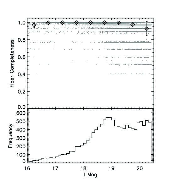
Figure 16.— Final AGES fiber completeness as a function of total $I$-band magnitude. This value represents the correction applied to each galaxy due to observed objects which did not receive a fiber due to fiber collisions as described in §A.2.

Figure 17.— Fraction of AGES targets which received redshifts as a function of the number of neighbor galaxies within 30” of the target’s location. The histogram (right axis) shows the distribution of neighbor counts for all of the AGES targets. When calculating the completeness correction for each galaxy in our survey we include the effects of neighboring galaxies as described in the text.

We would have preferred to define the fiber completeness more locally, e.g., count neighbors and find the fraction that got observed, as this would tie the incompleteness closer to the large-scale structure. This does not work because some rather isolated targets failed to get fibers, generally due to high over density elsewhere in the field, and so we are left with unobserved galaxies with undefined weights. This is only a problem in the less complete fields (13-15).

For redshift completeness, we are primarily concerned about trends with surface brightness. There are 274 primary galaxy targets (2.1%) that received a fiber but failed to get a redshift (of course, there are many more failed observations, but we reobserved most of them in order to get a useful redshift). We track the surface brightness by the $I$-band $1^{\prime\prime}$ aperture magnitude. In order to explore the redshift rate success, we apply three criteria to our sample:

1. Objects faintward of the main surface brightness locus as defined by $I_{\rm 1\farcs 0}-0.8I_{\rm tot}>7$, or not.

2. Objects whose colors suggest high redshift, $(R-I)-0.2(B_{W}-R)>0.55$, or not.

3. Objects that were sparse sampled.

Based on an object passing or failing each of these criteria, we derive 8 sets of objects. In each set, we bin the galaxies in 0.5 mag bins in aperture magnitude and consider the rate of getting a successful redshift (among the targets that received a fiber). Figure 18 shows the redshift completeness derived using this method as a function of the aperture magnitude of each AGES galaxy target. It is worth noting that we have not explicitly considered the signal-to-noise ratio of the observations in this spectral completeness model. In practice, some observations were better than others, and this would alter the angular structure of the corrections, but we believe this to be a minor effect.

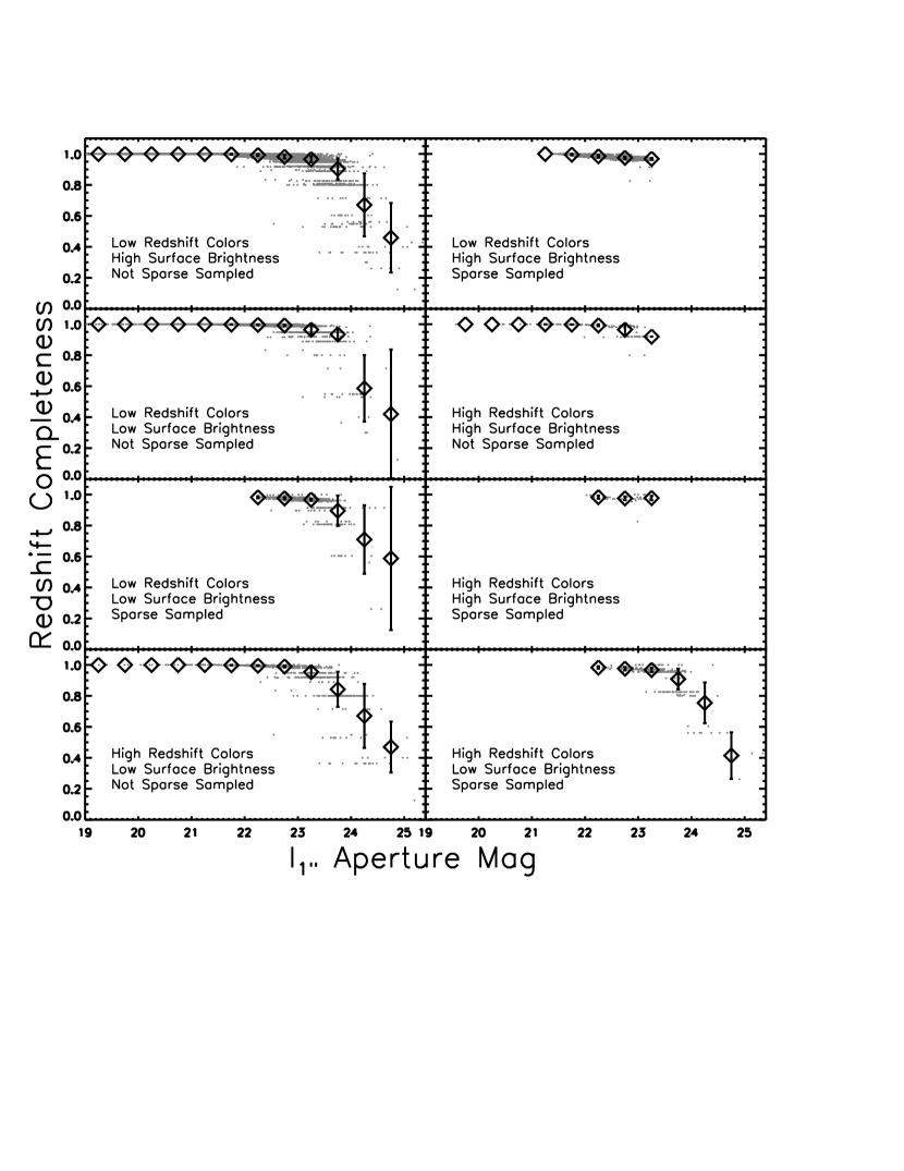
Figure 18.— Redshift completeness as a function of $I$-band aperture magnitude (measuring the flux contained within a Hectospec fiber). When calculating this completeness, we consider objects based on three criteria with limits described in the text. First, we separate galaxies based on their observed colors to separate galaxies with high- and low-redshift colors. We secondly divide the sample based on the surface brightness of each galaxy. Finally, we calculate the completeness separately for galaxies which were sparse sampled and those that were not. This separation gives rise to each of the 8 panels in the Figure. The subdivision of each sample is listed in the lower-left and the mean trend is showed by the diamonds with errorbars illustrating the 1-$\sigma$ range in values. When calculating the luminosity function, we utilize the raw completeness values in the figure; the means are shown to guide the eye.

Our final galaxy weight is calculating by multiplying the inverse of the sparse sampling rate, the fiber completeness, and the redshift completeness. Figure 19 illustrates the distribution of spectroscopic weight (the product of the fiber weight and redshift completeness weight) for the full galaxy sample as well as the red and blue galaxy samples separately. We have corrected for the photometric incompleteness by correcting the effective survey area as described above. In total, the main galaxy sample (after sparse sampling, area restrictions, and applying a $I_{\rm tot}<20.4$ flux limit) has 12,473 objects with good redshifts. Summing the weights yields 25,972 effective objects. This is in good agreement (0.3%) with the 26,033 targets in the parent $I_{\rm tot}<20.4$ sample after requiring good photometry in $B_{W}$, $R$, and $I$ and excluding bright stars from SDSS. These numbers do not match exactly because the sparse sampling was random and because of small unmodeled interactions between the various terms of the selection function (e.g., the fiber incompleteness differs slightly from one class of sparse-sampling to the next, but we have assumed the two independent when we multiply the corrections). The redshift distribution of AGES galaxies is shown in Figure 1.

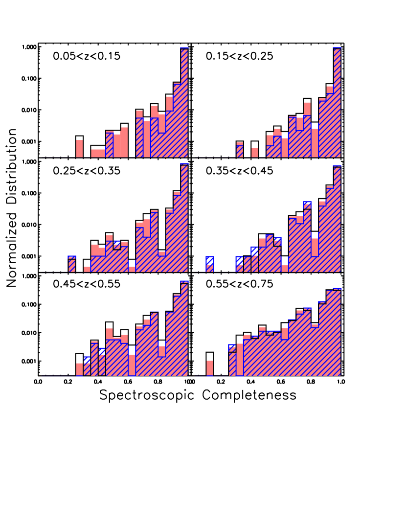
Figure 19.— Distribution of final spectroscopic completeness (not including corrections due to sparse sampling) for the full AGES galaxy sample. The empty histogram shows the full distribution of the sample. The filled histogram shows the distribution for red galaxies while the hashed histogram shows that for blue galaxies.

In summary, AGES successfully observed half of the total $I_{\rm tot}<20.4$ photometric sample in the Boötes field. Nearly all of this was due to the a priori sparse sampling which can be corrected exactly. The fiber incompleteness is 4.3% on average; the redshift incompleteness is 2.1%. Given the very high completeness, we are confident that the first-order attempts described above to correct the lingering incompleteness reduce the completeness uncertainties to well below the statistical uncertainties.

Table 1AGES ^0.1r-band $1/V_{\rm max}$ Luminosity Functions for All Galaxies

	Luminosity Function ($\times 10^{-4}$ $h^{3}$ Mpc-3 mag-1)
Luminosity Range	$0.05<z<0.15$	$0.15<z<0.25$	$0.25<z<0.35$	$0.35<z<0.45$	$0.45<z<0.55$	$0.55<z<0.75$
$-18.25<M<-18.00$	$140.82\pm 17.07$	$\cdots$	$\cdots$	$\cdots$	$\cdots$	$\cdots$
$-18.50<M<-18.25$	$133.97\pm 09.78$	$\cdots$	$\cdots$	$\cdots$	$\cdots$	$\cdots$
$-18.75<M<-18.50$	$113.45\pm 08.81$	$131.17\pm 05.82$	$\cdots$	$\cdots$	$\cdots$	$\cdots$
$-19.00<M<-18.75$	$106.26\pm 09.99$	$109.51\pm 04.64$	$\cdots$	$\cdots$	$\cdots$	$\cdots$
$-19.25<M<-19.00$	$119.46\pm 10.11$	$121.39\pm 18.13$	$\cdots$	$\cdots$	$\cdots$	$\cdots$
$-19.50<M<-19.25$	$106.22\pm 08.42$	$108.94\pm 04.67$	$\cdots$	$\cdots$	$\cdots$	$\cdots$
$-19.75<M<-19.50$	$92.76\pm 07.83$	$108.32\pm 04.80$	$\cdots$	$\cdots$	$\cdots$	$\cdots$
$-20.00<M<-19.75$	$88.19\pm 07.64$	$99.08\pm 04.45$	$70.31\pm 02.73$	$\cdots$	$\cdots$	$\cdots$
$-20.25<M<-20.00$	$90.35\pm 10.75$	$98.19\pm 04.80$	$58.42\pm 02.65$	$\cdots$	$\cdots$	$\cdots$
$-20.50<M<-20.25$	$52.88\pm 05.99$	$70.12\pm 03.68$	$56.53\pm 02.37$	$\cdots$	$\cdots$	$\cdots$
$-20.75<M<-20.50$	$49.64\pm 05.90$	$59.62\pm 03.39$	$45.67\pm 02.28$	$56.81\pm 01.86$	$\cdots$	$\cdots$
$-21.00<M<-20.75$	$38.72\pm 05.29$	$41.66\pm 03.59$	$34.54\pm 01.90$	$50.26\pm 01.76$	$\cdots$	$\cdots$
$-21.25<M<-21.00$	$30.29\pm 04.74$	$33.31\pm 02.53$	$29.82\pm 01.69$	$37.48\pm 01.52$	$\cdots$	$\cdots$
$-21.50<M<-21.25$	$20.45\pm 04.90$	$24.80\pm 02.18$	$18.55\pm 01.34$	$25.57\pm 01.26$	$29.04\pm 01.12$	$\cdots$
$-21.75<M<-21.50$	$12.68\pm 03.48$	$14.39\pm 01.66$	$11.06\pm 01.03$	$17.00\pm 01.01$	$24.08\pm 01.02$	$\cdots$
$-22.00<M<-21.75$	$5.75\pm 02.59$	$7.14\pm 01.17$	$7.20\pm 00.83$	$9.69\pm 00.76$	$13.61\pm 00.77$	$14.28\pm 00.61$
$-22.25<M<-22.00$	$4.77\pm 03.37$	$3.49\pm 00.82$	$3.61\pm 00.59$	$6.19\pm 00.61$	$9.22\pm 00.63$	$10.12\pm 00.49$
$-22.50<M<-22.25$	$26.57\pm 25.07$	$2.45\pm 00.69$	$1.66\pm 00.40$	$2.43\pm 00.38$	$5.23\pm 00.48$	$8.67\pm 00.46$
$-22.75<M<-22.50$	$0.67\pm 00.66$	$1.39\pm 00.52$	$0.77\pm 00.27$	$2.13\pm 00.36$	$2.40\pm 00.32$	$3.36\pm 00.28$
$-23.00<M<-22.75$	$0.69\pm 00.67$	$0.54\pm 00.47$	$0.19\pm 00.14$	$0.18\pm 00.10$	$1.41\pm 00.25$	$2.10\pm 00.22$

Table 2AGES ^0.1r-band $1/V_{\rm max}$ Luminosity Functions for Blue Galaxies

	Luminosity Function ($\times 10^{-4}$ $h^{3}$ Mpc-3 mag-1)
Luminosity Range	$0.05<z<0.15$	$0.15<z<0.25$	$0.25<z<0.35$	$0.35<z<0.45$	$0.45<z<0.55$	$0.55<z<0.75$
$-18.25<M<-18.00$	$123.12\pm 16.69$	$\cdots$	$\cdots$	$\cdots$	$\cdots$	$\cdots$
$-18.50<M<-18.25$	$113.97\pm 09.08$	$\cdots$	$\cdots$	$\cdots$	$\cdots$	$\cdots$
$-18.75<M<-18.50$	$84.64\pm 07.50$	$108.12\pm 05.36$	$\cdots$	$\cdots$	$\cdots$	$\cdots$
$-19.00<M<-18.75$	$75.80\pm 07.47$	$77.57\pm 03.93$	$\cdots$	$\cdots$	$\cdots$	$\cdots$
$-19.25<M<-19.00$	$87.82\pm 07.77$	$96.07\pm 17.99$	$\cdots$	$\cdots$	$\cdots$	$\cdots$
$-19.50<M<-19.25$	$68.98\pm 06.81$	$75.58\pm 03.92$	$\cdots$	$\cdots$	$\cdots$	$\cdots$
$-19.75<M<-19.50$	$61.50\pm 06.37$	$65.88\pm 03.64$	$\cdots$	$\cdots$	$\cdots$	$\cdots$
$-20.00<M<-19.75$	$51.44\pm 05.83$	$58.16\pm 03.35$	$47.53\pm 02.29$	$\cdots$	$\cdots$	$\cdots$
$-20.25<M<-20.00$	$45.16\pm 06.23$	$56.42\pm 03.68$	$31.45\pm 01.74$	$\cdots$	$\cdots$	$\cdots$
$-20.50<M<-20.25$	$27.14\pm 04.27$	$35.96\pm 02.63$	$34.90\pm 01.83$	$\cdots$	$\cdots$	$\cdots$
$-20.75<M<-20.50$	$22.75\pm 03.96$	$28.86\pm 02.36$	$24.46\pm 01.78$	$30.26\pm 01.35$	$\cdots$	$\cdots$
$-21.00<M<-20.75$	$17.45\pm 03.53$	$20.27\pm 02.96$	$16.18\pm 01.27$	$22.28\pm 01.17$	$\cdots$	$\cdots$
$-21.25<M<-21.00$	$10.34\pm 02.70$	$15.27\pm 01.71$	$13.55\pm 01.14$	$18.43\pm 01.07$	$\cdots$	$\cdots$
$-21.50<M<-21.25$	$9.38\pm 02.75$	$10.64\pm 01.43$	$7.92\pm 00.87$	$9.24\pm 00.75$	$13.59\pm 00.77$	$\cdots$
$-21.75<M<-21.50$	$3.47\pm 01.71$	$5.05\pm 00.98$	$5.14\pm 00.70$	$5.67\pm 00.58$	$9.17\pm 00.63$	$\cdots$
$-22.00<M<-21.75$	$0.70\pm 00.68$	$1.17\pm 00.48$	$2.66\pm 00.50$	$3.97\pm 00.49$	$4.57\pm 00.44$	$7.35\pm 00.45$
$-22.25<M<-22.00$	$2.43\pm 02.42$	$0.97\pm 00.43$	$0.69\pm 00.26$	$1.49\pm 00.30$	$3.06\pm 00.36$	$5.52\pm 00.39$
$-22.50<M<-22.25$	$0.69\pm 00.69$	$1.43\pm 00.52$	$0.31\pm 00.17$	$0.50\pm 00.17$	$0.94\pm 00.20$	$2.52\pm 00.26$
$-22.75<M<-22.50$	$0.67\pm 00.66$	$0.78\pm 00.39$	$0.29\pm 00.17$	$0.68\pm 00.20$	$0.64\pm 00.17$	$0.99\pm 00.16$
$-23.00<M<-22.75$	$0.69\pm 00.67$	$0.54\pm 00.47$	$\cdots$	$\cdots$	$0.18\pm 00.09$	$0.73\pm 00.15$

Table 3AGES ^0.1r-band $1/V_{\rm max}$ Luminosity Functions for Red Galaxies

	Luminosity Function ($\times 10^{-4}$ $h^{3}$ Mpc-3 mag-1)
Luminosity Range	$0.05<z<0.15$	$0.15<z<0.25$	$0.25<z<0.35$	$0.35<z<0.45$	$0.45<z<0.55$	$0.55<z<0.75$
$-18.25<M<-18.00$	$17.69\pm 03.59$	$\cdots$	$\cdots$	$\cdots$	$\cdots$	$\cdots$
$-18.50<M<-18.25$	$20.00\pm 03.63$	$\cdots$	$\cdots$	$\cdots$	$\cdots$	$\cdots$
$-18.75<M<-18.50$	$28.81\pm 04.63$	$23.05\pm 02.27$	$\cdots$	$\cdots$	$\cdots$	$\cdots$
$-19.00<M<-18.75$	$30.45\pm 06.64$	$31.94\pm 02.48$	$\cdots$	$\cdots$	$\cdots$	$\cdots$
$-19.25<M<-19.00$	$31.64\pm 06.46$	$25.32\pm 02.21$	$\cdots$	$\cdots$	$\cdots$	$\cdots$
$-19.50<M<-19.25$	$37.24\pm 04.96$	$33.36\pm 02.55$	$\cdots$	$\cdots$	$\cdots$	$\cdots$
$-19.75<M<-19.50$	$31.26\pm 04.55$	$42.45\pm 03.13$	$\cdots$	$\cdots$	$\cdots$	$\cdots$
$-20.00<M<-19.75$	$36.75\pm 04.94$	$40.92\pm 02.93$	$22.78\pm 01.48$	$\cdots$	$\cdots$	$\cdots$
$-20.25<M<-20.00$	$45.19\pm 08.76$	$41.77\pm 03.08$	$26.98\pm 02.00$	$\cdots$	$\cdots$	$\cdots$
$-20.50<M<-20.25$	$25.74\pm 04.19$	$34.15\pm 02.57$	$21.63\pm 01.51$	$\cdots$	$\cdots$	$\cdots$
$-20.75<M<-20.50$	$26.89\pm 04.37$	$30.76\pm 02.43$	$21.21\pm 01.43$	$26.55\pm 01.29$	$\cdots$	$\cdots$
$-21.00<M<-20.75$	$21.27\pm 03.94$	$21.39\pm 02.04$	$18.36\pm 01.42$	$27.98\pm 01.32$	$\cdots$	$\cdots$
$-21.25<M<-21.00$	$19.95\pm 03.89$	$18.04\pm 01.87$	$16.27\pm 01.25$	$19.05\pm 01.07$	$\cdots$	$\cdots$
$-21.50<M<-21.25$	$11.07\pm 04.06$	$14.16\pm 01.65$	$10.62\pm 01.01$	$16.33\pm 01.01$	$15.45\pm 00.82$	$\cdots$
$-21.75<M<-21.50$	$9.21\pm 03.03$	$9.35\pm 01.34$	$5.92\pm 00.75$	$11.33\pm 00.83$	$14.90\pm 00.80$	$\cdots$
$-22.00<M<-21.75$	$5.05\pm 02.50$	$5.97\pm 01.07$	$4.54\pm 00.66$	$5.72\pm 00.59$	$9.04\pm 00.63$	$8.16\pm 00.47$
$-22.25<M<-22.00$	$2.34\pm 02.34$	$2.51\pm 00.69$	$2.92\pm 00.53$	$4.70\pm 00.53$	$6.17\pm 00.52$	$5.52\pm 00.37$
$-22.50<M<-22.25$	$25.88\pm 25.06$	$1.02\pm 00.44$	$1.35\pm 00.36$	$1.93\pm 00.34$	$4.29\pm 00.43$	$6.56\pm 00.40$
$-22.75<M<-22.50$	$\cdots$	$0.61\pm 00.35$	$0.48\pm 00.21$	$1.46\pm 00.30$	$1.76\pm 00.28$	$2.53\pm 00.24$
$-23.00<M<-22.75$	$\cdots$	$\cdots$	$0.19\pm 00.14$	$0.18\pm 00.10$	$1.23\pm 00.23$	$1.49\pm 00.18$

Table 4$r^{0.1}$ Luminosity Function Parameters

Galaxy Sample	$z$	$M_{*}$	error	$\alpha$	$\phi_{*}$	% error	$j$	$\sigma_{\mbox{LSS}}$/$j$
					$h^{3}{\rm Mpc}^{-3}{\rm Mag}^{-1}$		$10^{8}hL_{\sun}{\rm Mpc}^{-3}$
All Galaxies	0.10	$-20.58$	0.05	$-1.05$	0.0159	11	$2.25\pm 0.65$	0.28
…	0.20	$-20.81$	0.04	$-1.05$	0.0152	5	$2.67\pm 0.56$	0.20
…	0.30	$-20.81$	0.03	$-1.05$	0.0124	7	$2.16\pm 0.39$	0.17
…	0.40	$-20.99$	0.04	$-1.05$	0.0144	7	$2.97\pm 0.45$	0.14
…	0.50	$-21.29$	0.08	$-1.05$	0.0108	10	$2.93\pm 0.41$	0.13
…	0.65	$-21.38$	0.06	$-1.05$	0.0105	14	$3.09\pm 0.36$	0.08
Blue Galaxies	0.10	$-20.31$	0.12	$-1.11$	0.0111	16	$1.27\pm 0.36$	0.28
…	0.20	$-20.57$	0.07	$-1.11$	0.0101	6	$1.49\pm 0.31$	0.20
…	0.30	$-20.54$	0.04	$-1.11$	0.0091	9	$1.29\pm 0.23$	0.17
…	0.40	$-20.78$	0.05	$-1.11$	0.0090	9	$1.59\pm 0.24$	0.14
…	0.50	$-20.93$	0.11	$-1.11$	0.0081	15	$1.65\pm 0.23$	0.13
…	0.65	$-21.13$	0.08	$-1.11$	0.0089	14	$2.17\pm 0.31$	0.08
Red Galaxies	0.10	$-20.49$	0.07	$-0.55$	0.0084	15	$0.93\pm 0.29$	0.28
…	0.20	$-20.63$	0.04	$-0.55$	0.0089	8	$1.12\pm 0.25$	0.20
…	0.30	$-20.74$	0.04	$-0.55$	0.0060	10	$0.84\pm 0.17$	0.17
…	0.40	$-20.84$	0.04	$-0.55$	0.0082	8	$1.26\pm 0.20$	0.14
…	0.50	$-21.19$	0.07	$-0.55$	0.0060	12	$1.28\pm 0.20$	0.13
…	0.65	$-21.46$	0.06	$-0.55$	0.0036	14	$0.97\pm 0.31$	0.30

Table 5$r^{0.1}$-band Evolution Parameters

Galaxy Sample	$Q$	$P$	$n$
	$M_{*}(z)=M_{*}(0)+Qz$	$\phi_{*}(z)\propto 1+Pz$	$\j_{{}^{0.1}r}(z)\propto(1+z)^{n}$
All Galaxies	$-1.67\pm 0.07$	$-0.59\pm 0.14$	$0.81\pm 0.27$
Blue Galaxies	$-1.66\pm 0.09$	$-0.38\pm 0.21$	$1.64\pm 0.39$
Red Galaxies	$-1.73\pm 0.07$	$-0.95\pm 0.10$	$0.54\pm 0.64$

Table 6AGES $B$-band $1/V_{\rm max}$ Luminosity Functions for All Galaxies

	Luminosity Function ($\times 10^{-4}$ $h^{3}$ Mpc-3 mag-1)
Luminosity Range	$0.05<z<0.15$	$0.15<z<0.25$	$0.25<z<0.35$	$0.35<z<0.45$	$0.45<z<0.55$	$0.55<z<0.75$
$-18.25<M<-18.00$	$107.74\pm 20.73$	$107.44\pm 19.41$	$\cdots$	$\cdots$	$\cdots$	$\cdots$
$-18.50<M<-18.25$	$100.15\pm 19.06$	$106.17\pm 16.21$	$\cdots$	$\cdots$	$\cdots$	$\cdots$
$-18.75<M<-18.50$	$71.43\pm 17.53$	$111.57\pm 13.54$	$\cdots$	$\cdots$	$\cdots$	$\cdots$
$-19.00<M<-18.75$	$62.89\pm 16.12$	$74.71\pm 11.31$	$\cdots$	$\cdots$	$\cdots$	$\cdots$
$-19.25<M<-19.00$	$52.47\pm 14.82$	$59.86\pm 09.45$	$\cdots$	$\cdots$	$\cdots$	$\cdots$
$-19.50<M<-19.25$	$60.86\pm 13.63$	$67.22\pm 07.89$	$73.83\pm 07.59$	$\cdots$	$\cdots$	$\cdots$
$-19.75<M<-19.50$	$41.44\pm 12.53$	$52.24\pm 06.59$	$57.96\pm 05.77$	$\cdots$	$\cdots$	$\cdots$
$-20.00<M<-19.75$	$26.88\pm 11.52$	$34.54\pm 05.51$	$46.85\pm 04.39$	$\cdots$	$\cdots$	$\cdots$
$-20.25<M<-20.00$	$22.89\pm 10.59$	$27.06\pm 04.60$	$34.76\pm 03.34$	$35.38\pm 04.47$	$\cdots$	$\cdots$
$-20.50<M<-20.25$	$25.35\pm 09.74$	$17.44\pm 03.84$	$23.18\pm 02.54$	$27.31\pm 03.19$	$\cdots$	$\cdots$
$-20.75<M<-20.50$	$5.68\pm 08.96$	$13.12\pm 03.21$	$16.41\pm 01.93$	$17.96\pm 02.27$	$\cdots$	$\cdots$
$-21.00<M<-20.75$	$3.72\pm 08.24$	$8.99\pm 02.68$	$9.80\pm 01.47$	$11.14\pm 01.62$	$14.63\pm 01.91$	$\cdots$
$-21.25<M<-21.00$	$7.40\pm 07.57$	$4.52\pm 02.24$	$4.61\pm 01.12$	$6.45\pm 01.16$	$9.64\pm 01.31$	$\cdots$
$-21.50<M<-21.25$	$4.03\pm 06.96$	$1.63\pm 01.87$	$2.69\pm 00.85$	$3.43\pm 00.83$	$5.17\pm 00.89$	$9.45\pm 00.67$
$-21.75<M<-21.50$	$0.10\pm 06.40$	$0.48\pm 01.56$	$0.73\pm 00.65$	$1.94\pm 00.59$	$2.77\pm 00.61$	$5.25\pm 00.50$
$-22.00<M<-21.75$	$\cdots$	$\cdots$	$0.38\pm 00.49$	$0.54\pm 00.42$	$0.86\pm 00.42$	$2.00\pm 00.37$
$-22.25<M<-22.00$	$1.98\pm 05.41$	$0.67\pm 01.09$	$\cdots$	$0.31\pm 00.30$	$0.31\pm 00.28$	$1.10\pm 00.28$

Table 7AGES $B$-band $1/V_{\rm max}$ Luminosity Functions for Red Galaxies

	Luminosity Function ($\times 10^{-4}$ $h^{3}$ Mpc-3 mag-1)
Luminosity Range	$0.05<z<0.15$	$0.15<z<0.25$	$0.25<z<0.35$	$0.35<z<0.45$	$0.45<z<0.55$	$0.55<z<0.75$
$-18.25<M<-18.00$	$79.30\pm 13.68$	$82.83\pm 09.09$	$\cdots$	$\cdots$	$\cdots$	$\cdots$
$-18.50<M<-18.25$	$75.34\pm 13.87$	$71.20\pm 07.79$	$\cdots$	$\cdots$	$\cdots$	$\cdots$
$-18.75<M<-18.50$	$47.95\pm 14.05$	$82.05\pm 06.68$	$\cdots$	$\cdots$	$\cdots$	$\cdots$
$-19.00<M<-18.75$	$35.01\pm 14.24$	$41.23\pm 05.72$	$\cdots$	$\cdots$	$\cdots$	$\cdots$
$-19.25<M<-19.00$	$29.74\pm 14.44$	$29.90\pm 04.90$	$\cdots$	$\cdots$	$\cdots$	$\cdots$
$-19.50<M<-19.25$	$36.16\pm 14.63$	$33.14\pm 04.20$	$42.71\pm 04.13$	$\cdots$	$\cdots$	$\cdots$
$-19.75<M<-19.50$	$15.53\pm 14.83$	$23.60\pm 03.60$	$32.19\pm 03.20$	$\cdots$	$\cdots$	$\cdots$
$-20.00<M<-19.75$	$11.74\pm 15.03$	$10.31\pm 03.09$	$22.35\pm 02.47$	$\cdots$	$\cdots$	$\cdots$
$-20.25<M<-20.00$	$6.70\pm 12.07$	$4.48\pm 02.65$	$14.69\pm 01.91$	$14.81\pm 02.43$	$\cdots$	$\cdots$
$-20.50<M<-20.25$	$13.09\pm 15.43$	$2.38\pm 02.27$	$8.06\pm 01.48$	$9.31\pm 01.79$	$\cdots$	$\cdots$
$-20.75<M<-20.50$	$0.57\pm 01.02$	$2.88\pm 01.94$	$4.56\pm 01.14$	$6.28\pm 01.31$	$\cdots$	$\cdots$
$-21.00<M<-20.75$	$0.37\pm 00.67$	$2.52\pm 01.67$	$3.12\pm 00.88$	$2.97\pm 00.97$	$7.46\pm 01.78$	$\cdots$
$-21.25<M<-21.00$	$3.21\pm 05.78$	$0.89\pm 01.43$	$1.29\pm 00.68$	$1.72\pm 00.71$	$5.02\pm 01.19$	$\cdots$
$-21.50<M<-21.25$	$4.03\pm 07.25$	$1.43\pm 01.22$	$1.03\pm 00.53$	$1.30\pm 00.52$	$2.71\pm 00.79$	$4.21\pm 00.67$
$-21.75<M<-21.50$	$0.01\pm 00.02$	$0.05\pm 00.09$	$0.44\pm 00.41$	$1.55\pm 00.39$	$1.67\pm 00.53$	$2.45\pm 00.48$
$-22.00<M<-21.75$	$\cdots$	$\cdots$	$0.23\pm 00.32$	$0.48\pm 00.28$	$0.79\pm 00.35$	$1.33\pm 00.35$
$-22.25<M<-22.00$	$0.20\pm 00.36$	$0.67\pm 00.77$	$\cdots$	$0.15\pm 00.21$	$0.31\pm 00.23$	$0.77\pm 00.25$

Table 8AGES $B$-band $1/V_{\rm max}$ Luminosity Functions for Blue Galaxies

	Luminosity Function ($\times 10^{-4}$ $h^{3}$ Mpc-3 mag-1)
Luminosity Range	$0.05<z<0.15$	$0.15<z<0.25$	$0.25<z<0.35$	$0.35<z<0.45$	$0.45<z<0.55$	$0.55<z<0.75$
$-18.25<M<-18.00$	$28.44\pm 07.85$	$24.62\pm 09.22$	$\cdots$	$\cdots$	$\cdots$	$\cdots$
$-18.50<M<-18.25$	$24.81\pm 07.96$	$34.97\pm 07.90$	$\cdots$	$\cdots$	$\cdots$	$\cdots$
$-18.75<M<-18.50$	$23.48\pm 08.07$	$29.52\pm 06.77$	$\cdots$	$\cdots$	$\cdots$	$\cdots$
$-19.00<M<-18.75$	$27.88\pm 08.17$	$33.48\pm 05.80$	$\cdots$	$\cdots$	$\cdots$	$\cdots$
$-19.25<M<-19.00$	$22.73\pm 08.28$	$29.96\pm 04.97$	$\cdots$	$\cdots$	$\cdots$	$\cdots$
$-19.50<M<-19.25$	$24.69\pm 08.40$	$34.08\pm 04.26$	$31.11\pm 04.83$	$\cdots$	$\cdots$	$\cdots$
$-19.75<M<-19.50$	$25.90\pm 08.51$	$28.64\pm 03.65$	$25.77\pm 03.74$	$\cdots$	$\cdots$	$\cdots$
$-20.00<M<-19.75$	$15.14\pm 08.62$	$24.22\pm 03.13$	$24.50\pm 02.89$	$\cdots$	$\cdots$	$\cdots$
$-20.25<M<-20.00$	$16.18\pm 08.74$	$22.59\pm 02.68$	$20.08\pm 02.23$	$20.56\pm 02.86$	$\cdots$	$\cdots$
$-20.50<M<-20.25$	$12.26\pm 08.86$	$15.06\pm 02.30$	$15.12\pm 01.73$	$18.00\pm 02.10$	$\cdots$	$\cdots$
$-20.75<M<-20.50$	$5.11\pm 08.98$	$10.24\pm 01.97$	$11.85\pm 01.33$	$11.69\pm 01.55$	$\cdots$	$\cdots$
$-21.00<M<-20.75$	$3.34\pm 09.10$	$6.46\pm 01.69$	$6.68\pm 01.03$	$8.17\pm 01.14$	$7.18\pm 01.45$	$\cdots$
$-21.25<M<-21.00$	$4.19\pm 09.22$	$3.63\pm 01.45$	$3.33\pm 00.80$	$4.73\pm 00.84$	$4.62\pm 00.97$	$\cdots$
$-21.50<M<-21.25$	$\cdots$	$0.21\pm 01.24$	$1.67\pm 00.62$	$2.14\pm 00.62$	$2.46\pm 00.64$	$6.28\pm 00.57$
$-21.75<M<-21.50$	$0.09\pm 09.47$	$0.43\pm 01.06$	$0.29\pm 00.48$	$0.39\pm 00.45$	$1.10\pm 00.43$	$3.35\pm 00.41$
$-22.00<M<-21.75$	$\cdots$	$\cdots$	$0.15\pm 00.37$	$0.05\pm 00.33$	$0.07\pm 00.29$	$0.81\pm 00.29$
$-22.25<M<-22.00$	$1.78\pm 09.73$	$\cdots$	$\cdots$	$0.16\pm 00.25$	$0.01\pm 00.19$	$0.39\pm 00.21$

Table 9$B$-band Luminosity Function Parameters

Galaxy Sample	$z$	$M_{*}$	error	$\alpha$	$\phi_{*}$	% error	$j$	$\sigma_{\mbox{LSS}}$/$j$
					$10^{-3}h^{3}{\rm Mpc}^{-3}{\rm Mag}^{-1}$		$10^{8}hL_{\sun}{\rm Mpc}^{-3}$
All Galaxies	0.10	-19.92	0.05	-1.20	8.41	10	$1.58\pm 0.50$	0.28
…	0.20	-20.04	0.04	-1.20	8.97	4	$1.88\pm 0.46$	0.20
…	0.30	-20.05	0.04	-1.20	10.84	8	$2.30\pm 0.34$	0.17
…	0.40	-20.25	0.04	-1.20	8.69	7	$2.22\pm 0.38$	0.14
…	0.50	-20.44	0.08	-1.20	7.95	10	$2.40\pm 0.35$	0.13
Blue Galaxies	0.10	-19.65	0.12	-1.30	6.03	16	$0.89\pm 0.32$	0.28
…	0.20	-19.77	0.09	-1.30	6.52	5	$1.07\pm 0.29$	0.20
…	0.30	-19.90	0.04	-1.30	5.74	8	$1.06\pm 0.23$	0.17
…	0.40	-20.05	0.07	-1.30	6.73	10	$1.42\pm 0.23$	0.14
…	0.50	-20.26	0.13	-1.30	6.47	14	$1.66\pm 0.21$	0.13
Red Galaxies	0.10	-19.63	0.09	-0.50	6.94	16	$0.68\pm 0.17$	0.28
…	0.20	-19.67	0.06	-0.50	8.42	7	$0.86\pm 0.16$	0.20
…	0.30	-19.72	0.05	-0.50	7.91	10	$0.85\pm 0.11$	0.17
…	0.40	-19.81	0.06	-0.50	7.44	8	$0.86\pm 0.12$	0.14
…	0.50	-19.89	0.08	-0.50	6.09	10	$0.76\pm 0.13$	0.13

Table 10AGES Galaxy Selection Criteria and Sparse Sampling Rates

Sample Name	gshort Bit	Bright Sample Limits	Faint Sample Limits	Faint Sample Sparse Sampling Rate
Main $I$-band Sample	4096	$15.45<I<18.95$	$18.95<I<20.45$	20%
$R$-band Sample	1024	$R\leq 19.41$	$19.41\leq R\leq 20.21$	20%
$B_{w}$-band Sample	512	$B_{w}\leq 20.5$	$20.5\leq B_{w}\leq 21.3$	20%
$J$-band Sample	256	$J\leq 18.42$	$18.42\leq J\leq 19.42$	20%
$K_{s}$-band Sample	128	$K_{s}\leq 17.84$	$17.84\leq K_{s}\leq 18.34$	20%
GALEX NUV Sample	64	$NUV<21$	$21<NUV<22$	30%
GALEX FUV Sample	32	$FUV<22$	$22<FUV<22.5$	30%
3.6$\mu$m Sample	16	$[3.6\mu m]<18$	$18\leq[3.6\mu m]\leq 18.5$	30%
4.5$\mu$m Sample	8	$[4.5\mu m]<18.46$	$18.46\leq[4.5\mu m]\leq 18.96$	30%
5.8$\mu$m Sample	4	$[5.8\mu m]<18.43$	$18.43\leq[5.8\mu m]\leq 18.93$	30%
8.0$\mu$m sample	2	$[8.0\mu m]<18.2$	$18.2\leq[8.0\mu m]\leq 18.8$	30%
MIPS 24$\mu$m Sample	1	$F_{24}\geq 0.5$ mJy	$0.3{\rm mJy}\leq F_{24}<0.5{\rm mJy}$	30%

.

Table 11AGES Main Galaxy Subsample Statistics

Sample Name	Sampling Rate	Targets	Spectra	Redshifts	Completeness
MIPS	30%	4662	4484	4411	95%
IRAC [8.0]	30%	3536	3498	3490	99%
IRAC [5.8]	30%	4058	3982	3927	98%
IRAC [4.5]	30%	6215	6081	5999	98%
IRAC [3.6]	30%	4992	4882	4792	98%
GALEX FUV	30%	545	422	520	96%
GALEX NUV	30%	1836	1779	1775	97%
K-band	20%	5399	5314	5302	98%
J-band	20%	4319	4288	4278	98%
B-band	20%	4345	4278	4237	99%
R-band	20%	7480	7378	7304	99%
Other I-band	…	18368	8257	7727	42%
Main I-band	20%	11011	10640	10306	94%

References

- Assef et al. (2008) Assef, R. J., et al. 2008, ApJ, 676, 286
- Assef et al. (2010) Assef, R. J., et al. 2010, ApJ, 713, 970
- Bell et al. (2004) Bell, E. F., et al. 2004, ApJ, 608, 752
- Bertin & Arnouts (1996) Bertin, E., & Arnouts, S. 1996, A&AS, 117, 393
- Blanton et al. (2001) Blanton, M. R., et al. 2001, AJ, 121, 2358
- Blanton et al. (2003) Blanton, M. R., et al. 2003, ApJ, 592, 819
- Blanton et al. (2005) Blanton, M. R., et al. 2005, AJ, 129, 2562
- Blanton & Roweis (2007) Blanton, M. R., & Roweis, S. 2007, AJ, 133, 734
- Brinchmann et al. (1998) Brinchmann, J., et al. 1998, ApJ, 499, 112
- Brand et al. (2009) Brand, K., et al. 2009, ApJ, 693, 340
- Brown et al. (2007) Brown, M. J. I., Dey, A., Jannuzi, B. T., Brand, K., Benson, A. J., Brodwin, M., Croton, D. J., & Eisenhardt, P. R. 2007, ApJ, 654, 858
- Brown et al. (2009) Brown, M. J. I., et al. 2009, ApJ, 703, 150
- Cohen (2002) Cohen, J. G. 2002, ApJ, 567, 672
- Colless et al. (2001) Colless, M., et al. 2001, MNRAS, 328, 1039
- Cool (2007) Cool, R. J. 2007, ApJS, 169, 21
- Cowie et al. (1996) Cowie, L. L., Songaila, A., Hu, E. M., & Cohen, J. G. 1996, AJ, 112, 839
- Cross et al. (2004) Cross, N. J. G., et al. 2004, AJ, 128, 1990
- Croton et al. (2005) Croton, D. J., et al. 2005, MNRAS, 356, 1155
- Davis & Huchra (1982) Davis, M., & Huchra, J. 1982, ApJ, 254, 437
- Davis et al. (2003) Davis, M., et al. 2003, Proc. SPIE, 4834, 161
- de Lapparent et al. (2003) de Lapparent, V., Galaz, G., Bardelli, S., & Arnouts, S. 2003, A&A, 404, 831
- Eales (1993) Eales, S. 1993, ApJ, 404, 51
- Ellis et al. (1996) Ellis, R. S., Colless, M., Broadhurst, T., Heyl, J., & Glazebrook, K. 1996, MNRAS, 280, 235
- Efstathiou et al. (1988) Efstathiou, G., Ellis, R. S., & Peterson, B. A. 1988, MNRAS, 232, 431
- Fabricant et al. (1998) Fabricant, D. G., Hertz, E. N., Szentgyorgyi, A. H., Fata, R. G., Roll, J. B., & Zajac, J. M. 1998, Proc. SPIE, 3355, 285
- Fabricant et al. (2005) Fabricant, D., et al. 2005, PASP, 117, 1411
- Faber et al. (2007) Faber, S. M., et al. 2007, ApJ, 665, 265
- Fukugita et al. (1996) Fukugita, M., Ichikawa, T., Gunn, J. E., Doi, M., Shimasaku, K., & Schneider, D. P. 1996, AJ, 111, 1748
- Heyl et al. (1997) Heyl, J., Colless, M., Ellis, R. S., & Broadhurst, T. 1997, MNRAS, 285, 613
- Hickox et al. (2009) Hickox, R. C., et al. 2009, ApJ, 696, 891
- Huchra et al. (1983) Huchra, J., Davis, M., Latham, D., & Tonry, J. 1983, ApJS, 52, 89
- Ilbert et al. (2006) Ilbert, O., et al. 2006, A&A, 453, 809
- Im et al. (2002) Im, M., et al. 2002, ApJ, 571, 136
- Jannuzi & Dey (1999) Jannuzi, B. T., & Dey, A. 1999, ASP Conf. Ser. 191: Photometric Redshifts and the Detection of High Redshift Galaxies, 191, 111
- Kochanek et al. (2001) Kochanek, C. S., et al. 2001, ApJ, 560, 566
- Kochanek et al. (2011) Kochanek, C. S., Eisenstein, D. J., Cool, R. J., et al. 2011, arXiv:1110.4371
- Kron (1980) Kron, R. G. 1980, ApJS, 43, 305
- Le Fèvre et al. (2004) Le Fèvre, O., et al. 2004, A&A, 428, 1043
- Lilly et al. (1995) Lilly, S. J., Tresse, L., Hammer, F., Crampton, D., & Le Fevre, O. 1995, ApJ, 455, 108
- Lin et al. (1999) Lin, H., Yee, H. K. C., Carlberg, R. G., Morris, S. L., Sawicki, M., Patton, D. R., Wirth, G., & Shepherd, C. W. 1999, ApJ, 518, 533
- Madgwick et al. (2002) Madgwick, D. S., et al. 2002, MNRAS, 333, 133
- Montero-Dorta & Prada (2009) Montero-Dorta, A. D., & Prada, F. 2009, MNRAS, 399, 1106
- Norberg et al. (2002) Norberg, P., et al. 2002, MNRAS, 336, 907
- Oke (1974) Oke, J. B. 1974, ApJS, 27, 21
- Pozzetti et al. (2003) Pozzetti, L., et al. 2003, A&A, 402, 837
- Roll et al. (1998) Roll, J. B., Fabricant, D. G., & McLeod, B. A. 1998, Proc. SPIE, 3355, 324
- Sandage et al. (1979) Sandage, A., Tammann, G. A., & Yahil, A. 1979, ApJ, 232, 352
- Schechter (1976) Schechter, P. 1976, ApJ, 203, 297
- Spergel et al. (2007) Spergel, D. N., et al. 2007, ApJS, 170, 377
- Strauss et al. (2002) Strauss, M. A., et al. 2002, AJ, 124, 1810
- Takeuchi et al. (2000) Takeuchi, T. T., Yoshikawa, K., & Ishii, T. T. 2000, ApJS, 129, 1
- Willmer et al. (2006) Willmer, C. N. A., et al. 2006, ApJ, 647, 853
- Wolf et al. (2003) Wolf, C., Meisenheimer, K., Rix, H.-W., Borch, A., Dye, S., & Kleinheinrich, M. 2003, A&A, 401, 73
- York et al. (2000) York, D. G., et al. 2000, AJ, 120, 1579