Large-scale 3D MHD simulation on the solar flux emergence and the small-scale dynamic features in an active region

We have performed a three-dimensional magnetohydrodynamic simulation to study the emergence of a twisted magnetic flux tube from $-20,000\ {\rm km}$ of the solar convection zone to the corona through the photosphere and the chromosphere. The middle part of the initial tube is endowed with a density deficit to instigate a buoyant emergence. As the tube approaches the surface, it extends horizontally and makes a flat magnetic structure due to the photosphere ahead of the tube. Further emergence to the corona breaks out via the interchange-mode instability of the photospheric fields, and eventually several magnetic domes build up above the surface. What is new in this three-dimensional experiment is, multiple separation events of the vertical magnetic elements are observed in the photospheric magnetogram, and they reflect the interchange instability. Separated elements are found to gather at the edges of the active region. These gathered elements then show shearing motions. These characteristics are highly reminiscent of active region observations. On the basis of the simulation results above, we propose a theoretical picture of the flux emergence and the formation of an active region that explains the observational features, such as multiple separations of faculae and the shearing motion.

1 Introduction

Solar active regions including sunspots are generally thought to be the consequence of the magnetic flux emergence (Parker 1955). Observationally, they appear as a developing bipolar pair in the photospheric magnetogram and arch-filament system in H$\alpha$ (Zwaan 1985). Strous et al. (1996) and Strous & Zwaan (1999) find the hierarchy of motions of magnetic elements in the active region: faculae of positive and negative polarities separate from each other toward the edges of the region, while pores of each polarity move along the edges toward the major sunspots.

Dynamics of the flux emergence have been studied widely through extensive numerical simulations, both in two and three dimensions (e.g. Shibata et al. 1989; Fan 2001; Archontis et al. 2004). It has been shown that the flux tube rises due to the Parker instability (Parker 1966) and expands into the corona in a self-similar way, which explains the characteristics of the flux emergence such as $\Omega$-shaped loops and the downflows at the footpoints of the loops.

In this paper, we report first results of the large-scale three-dimensional magnetohydrodynamic (3D MHD) simulation on the emergence of a twisted flux tube from a deeper convection zone ($-20,000\ {\rm km}$) into the corona through the photosphere. In our previous 2D experiments, Toriumi & Yokoyama (2010) and Toriumi & Yokoyama (2011) (hereafter papers I and II, respectively), we found the conditions of the magnetic flux for reasonable emergence such as the field strength, the total flux, and the twist of the tube at a depth of $-20,000\ {\rm km}$. We apply these values as the initial conditions in the 3D calculation. As a result, several characteristics are found to be consistent with the previous 2D experiments and observations. On the basis of this simulation, we also suggest a new theoretical picture of the flux emergence and the birth of an active region through the surface.

2 Numerical Setup

The basic MHD equations solved in this simulation in vector form are as follows:

$$\frac{\partial\rho}{\partial t}+\mbox{\boldmath$\nabla$}\cdot(\rho\mbox{\boldmath$V$})=0,$$ (1)

$$\frac{\partial}{\partial t}(\rho\mbox{\boldmath$V$})+\mbox{\boldmath$\nabla$}\cdot\left(\rho\mbox{\boldmath$V$}\mbox{\boldmath$V$}+p\mbox{\boldmath$I$}-\frac{\mbox{\boldmath$BB$}}{4\pi}+\frac{\mbox{\boldmath$B$}^{2}}{8\pi}\mbox{\boldmath$I$}\right)-\rho\mbox{\boldmath$g$}=0,$$ (2)

$$\frac{\partial\mbox{\boldmath$B$}}{\partial t}=\mbox{\boldmath$\nabla$}\times(\mbox{\boldmath$V$}\times\mbox{\boldmath$B$}),$$ (3)

$$\frac{\partial}{\partial t}\left(\rho U+\frac{1}{2}\rho\mbox{\boldmath$V$}^{2}+\frac{\mbox{\boldmath$B$}^{2}}{8\pi}\right)$$

$$+\mbox{\boldmath$\nabla$}\cdot\left[\left(\rho U+p+\frac{1}{2}\rho\mbox{\boldmath$V$}^{2}\right)\mbox{\boldmath$V$}+\frac{c}{4\pi}\mbox{\boldmath$E$}\times\mbox{\boldmath$B$}\right]-\rho\mbox{\boldmath$g$}\cdot\mbox{\boldmath$V$}=0,$$ (4)

and

$$U=\frac{1}{\gamma-1}\frac{p}{\rho},$$ (5)

$$\mbox{\boldmath$E$}=-\frac{1}{c}\mbox{\boldmath$V$}\times\mbox{\boldmath$B$},$$ (6)

$$p=\frac{k_{\rm B}}{m}\rho T,$$ (7)

where $U$ is the internal energy per unit mass, $I$ the unit tensor, $k_{\rm B}$ the Boltzmann constant, $m$ the mean molecular mass, and $g$ the uniform gravitational acceleration. Other symbols have their usual meanings: $\rho$ is for density, $V$ velocity vector, $p$ pressure, $B$ magnetic field, $c$ speed of light, $E$ electric field, and $T$ temperature. Here, the medium is assumed to be an inviscid perfect gas with a specific heat ratio $\gamma=5/3$. The equations are normalized by the pressure scale height $H_{0}=200\ {\rm km}$ for length, sound speed $C_{\rm s0}=8\ {\rm km\ s}^{-1}$ for velocity, $\tau_{0}\equiv H_{0}/C_{\rm s0}=25\ {\rm s}$ for time, $\rho_{0}=1.4\times 10^{-7}\ {\rm g\ cm}^{-3}$ for density, all of which are typical values for the photosphere. The units for pressure, temperature, and magnetic field strength are $p_{0}=9.0\times 10^{4}\ {\rm dyn\ cm}^{-2}$, $T_{0}=4000\ {\rm K}$, and $B_{0}=300\ {\rm G}$, respectively.

In this experiment, we set 3D Cartesian coordinates $(x,y,z)$, where $z$ is parallel to the gravitational acceleration, i.e., $\mbox{\boldmath$g$}=(0,0,-g_{0})$. The numerical domain is $(-400,-200,-200)\leq(x/H_{0},y/H_{0},z/H_{0})\leq(400,200,250)$ and the total grid number is $1602\times 256\times 1024$. The grid spacing for $x$-direction is $\Delta x/H_{0}=0.5$ (uniform); for the other directions, $\Delta y/H_{0}=0.5$ and $\Delta z/H_{0}=0.2$ at the central area of the domain, which gradually increase for each direction. We assume periodic boundaries for both horizontal directions and symmetric boundaries for the vertical direction.

The background stratification consists of the adiabatically stratified convective layer ($z/H_{0}<0$), the cool isothermal ($T(z)/T_{0}=1$) photosphere/chromosphere ($0\leq z/H_{0}<10$), and the hot isothermal ($T(z)/T_{0}=100$) corona ($z/H_{0}>10$). Here, the photosphere is isothermally stratified, i.e., convectively stable against the rising motion of the plasma. A transition region connects the low- and high-temperature atmospheres with a steep temperature gradient at around $z/H_{0}=10$. The initial flux tube embedded at $z=-100H_{0}=-20,000\ {\rm km}$ is uniformly twisted, i.e., $B_{\phi}(r)=qrB_{x}(r)$, where $B_{x}(r)=B_{\rm tube}\exp{(-r^{2}/R_{\rm tube}^{2})}$ is the axial field, $r$ the radial distance from the axis, $B_{\rm tube}=67B_{0}=2.0\times 10^{4}\ {\rm G}$ the field strength at the axis, $R_{\rm tube}=5H_{0}=1000\ {\rm km}$ the typical tube radius, $B_{\phi}(r)$ the azimuthal component, and $q$ the twist parameter which is set to be $0.1/H_{0}=5.0\times 10^{-4}\ {\rm km}^{-1}$ (stable to the kink instability). The total flux of the axial component is $\Phi=6.3\times 10^{20}\ {\rm Mx}$. The middle of the tube around $x/H_{0}=0$ is made buoyant through thermal equilibrium between the inside and the outside of the tube, and the buoyancy decreases as a function of the form $\exp(-x^{2}/\lambda^{2})$, where $\lambda/H_{0}=400$. The tube strength, the total flux, and the twist are chosen to satisfy the conditions found in papers I and II. The initial background distribution of gas pressure, density, and temperature, and the magnetic pressure are indicated in Figure 1(a). The density inside and outside the tube along $x$-axis are shown in Figure 1(b). One can see that, although the density is reduced throughout the whole tube, the middle part is most buoyant.

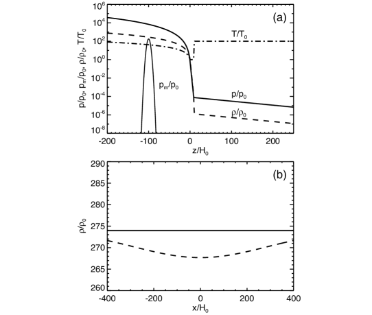
Figure 1: (a) One-dimensional ($z$-)distributions of the initial background gas pressure (thick solid line), density (dashed line), and temperature (dash-dotted line). The magnetic pressure $p_{\rm m}=B^{2}/(8\pi)$ along the vertical axis $x/H_{0}=y/H_{0}=0$ is overplotted with a thin solid line. (b) Background density profile at $z=-100H_{0}$ (solid line). Density inside the tube along $(y,z)=(0,-100H_{0})$ is overplotted with dashed line.

3 Results

3.1 General Evolution

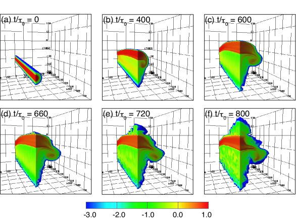
Figure 2: Time-evolution of the twisted emerging flux tube. Logarithmic field strength $\log_{10}(|B|/B_{0})$ for six different times in a limited region ($x/H_{0}<0,y/H_{0}>0$) is shown. The level of $z/H_{0}=0$ corresponds to the boundary between the convection zone and the photosphere.

Figure 2 shows the time evolution of the emerging twisted flux tube. Here, the logarithmic field strength $\log_{10}{(|B|/B_{0})}$ only in the region $x/H_{0}\leq 0$ and $y/H_{0}\geq 0$ is plotted. At $t/\tau_{0}=0$ (Fig. 2(a)), the initial tube is placed at $z/H_{0}=-100$. Due to the buoyancy of the tube itself, it rises through the convection zone ($t/\tau_{0}=400$, see Fig. 2(b)). The tube expands as the external density decreases with height. While the plasma draining from the apex to both feet accelerates the rising tube, the aerodynamic drag decelerates the tube, since the external flow around the cross-section forms a wake behind the main tube. One can see a vortex roll at the flank of the tube and an elongated tail below. However, the azimuthal component of the flux tube yields the inward curvature force to maintain the tube coherent. The upper surface of the rising tube becomes fluted due to the interchange-mode of the magnetic buoyancy instability (magnetic Rayleigh-Taylor instability). Figure 3 is a two-dimensional ($x$–$z$) slice of the rising flux tube, which shows the fluting at the top of the tube. The rise velocity levels off while in the middle of the convection zone.

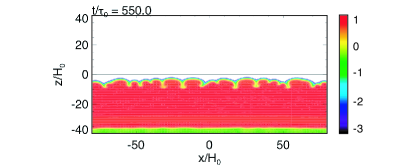
Figure 3: Two-dimensional ($x$–$z$) closeup of the rising flux tube at $t/\tau_{0}=550$. Logarithmic field strength $\log_{10}(|B|/B_{0})$ is plotted, while the photospheric height $z/H_{0}=0$ is indicated with a solid line.

Approaching the surface at $t/\tau_{0}=600$ in Fig. 2(c), the tube decelerates and expands laterally in the $y$-direction to make a flat structure just beneath the photosphere ($60\ {\rm Mm}\times 20\ {\rm Mm}$). The deceleration and the flattening occur because the plasma between the rising tube and the convectively stable photosphere is compressed, which in turn suppresses the rising tube from below. It should be noted that the deceleration and the flat magnetic structure are consistent with the previous 2D experiments (papers I and II). Here, the outermost field lines of the flat tube, i.e., fields at the surface are mostly in the negative $y$-direction.

As the surficial field strength increases to satisfy the criterion for the interchange-mode of magnetic buoyancy instability (e.g. Newcomb 1961), the secondary evolution to the upper atmosphere takes place at around $t/\tau_{0}=660$ (Fig. 2(d)). We find that several magnetic domes have been built in the central area around $x/H_{0}=y/H_{0}=0$ at this stage, aligned in the $x$-direction, each being directed in the $y$-direction. As the central domes develop, another several domes are newly created beside the central ones ($t/\tau_{0}=750$; Fig. 2(e)). The domes continue growing and merge with each other in the corona. After $t/\tau_{0}=700$, the rising velocity declines again, and eventually the emerging flux reaches $z/H_{0}\sim 35$ at $t/\tau_{0}=800$ (Fig. 2(f)). The subsurface structure extends $-200<x/H_{0}<200$ and $-40<y/H_{0}<40$.

The whole evolution process is the same as the “two-step emergence” model observed in the 2D experiments (papers I and II). However, the final height of the coronal structure is different from the 2D cases: the height in the present calculation is only $z/H_{0}=35$, while the fluxes in 2D were more than 200. The difference occurs due to the three-dimensionality. That is, in the 2D simulations, the magnetic pressure expands the magnetic flux only in the $(x,z)$ or $(y,z)$ plane. In the 3D case, however, the magnetic pressure inflates the flux in all $(x,y,z)$ directions, which results in lower magnetic domes. This 3D situation is the same as the free expansion regime by Matsumoto et al. (1993).

3.2 Magnetic Structures in the Photosphere

Figure 4 shows the vertical field strength ($B_{z}/B_{0}$; magnetogram) and the corresponding vertical velocity ($V_{z}/C_{\rm s0}$; Dopplergram) with the horizontal velocity field ($V_{\rm h}/C_{\rm s0}$) at the surface $z/H_{0}=0$ at $t/\tau_{0}=660$ and 800. In the Dopplergram, red indicates a downward motion ($V_{z}/C_{\rm s0}<0$). At $t/\tau_{0}\sim 610$, we observe that some blueshifts and divergent flows appear before the flux emergence, which indicates that the compressed plasma between the rising tube and the photosphere escapes laterally at the surface.

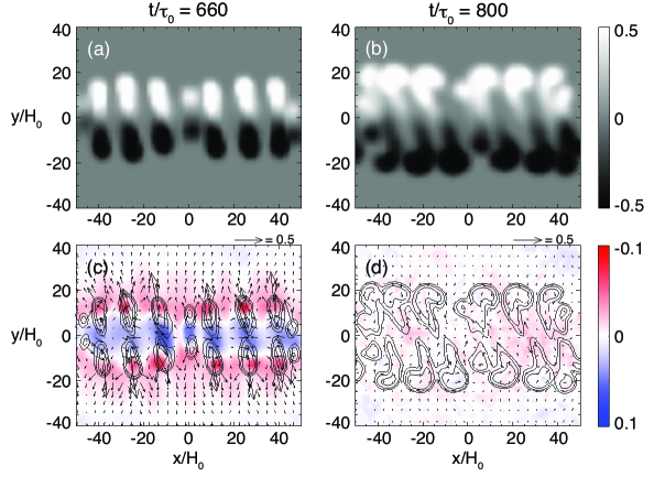
Figure 4: (Top) Time-evolution of vertical magnetic field strength $B_{z}/B_{0}$ at the surface $z/H_{0}=0$ (magnetogram). White (black) indicates the positive (negative) polarity. (Bottom) Corresponding velocity fields (Dopplergram). The vertical velocity $V_{z}/C_{\rm s0}$ (color; red is downward) and the horizontal velocity $V_{\rm h}/C_{\rm s0}$ (arrows) are shown. Corresponding vertical field $B_{z}/B_{0}$ at the photosphere is over-plotted with contours.

At $t/\tau_{0}=660$, in Fig. 4(a), magnetic elements of positive and negative polarities emerge onto the surface. The absolute field strength of each polarity is more than a hundred Gauss. In Fig. 4(c), one can find the blueshifts of the order of a few ${\rm km\ s}^{-1}$ between each pair and the redshifts up to $0.12C_{\rm s0}=1\ {\rm km\ s}^{-1}$ in the core of each patch. At this time, the horizontal speed in the positive and negative polarities is at its peak ($4$–$8\ {\rm km\ s}^{-1}$), showing separative motions. These features indicate that the magnetic flux emerges upward, while the plasma drains downward to both footpoints along the field lines. Here, the surface field is mostly directed in the negative $y$-direction, and the wavelengths are $\lambda_{\parallel}\sim 20H_{0}$ and $\lambda_{\perp}\sim 15H_{0}$ respectively, where $\lambda_{\parallel}$ and $\lambda_{\perp}$ are the wavelengths parallel and perpendicular to the surface horizontal field. The parallel wavelength $\lambda_{\parallel}\sim 20H_{0}$ is the most unstable wavelength of the linear Parker instability at the photosphere.

We speculate that the wavelength perpendicular to the field $\lambda_{\perp}$ is determined by the wavelength of the interchange-mode instability of the flux tube before it reaches the surface. During its ascent within the convection zone, the surface of the flux tube is found to be fluted due to the interchange instability (see Sect. 3.1). When the density smoothly increases upward between the magnetized and the unmagnetized atmosphere, the growth rate of the interchange instability levels off as the wavenumber increases, and the typical wavenumber of this saturation is approximately an inverse of the density transition scale (Chandrasekhar 1961). Considering the original tube is assumed to have a Gaussian profile, i.e., $B_{x}(r)=B_{\rm tube}\exp{(-r^{2}/R_{\rm tube}^{2})}$, and thus the density transition is also a function of $\exp{(-r^{2}/R_{\rm tube}^{2})}$, the scale of this transition layer is $\sim R_{\rm tube}$. Therefore, the wavelength of this instability within the convection zone is approximately several times the original tube’s radius ($R_{\rm tube}=5H_{0}$), which results in the wavelength of the secondary emergence $\lambda_{\perp}\sim 15H_{0}$ at the photosphere.

At $t/\tau_{0}=800$, the magnetic pairs develop and the region extends $-120<x/H_{0}<120$ and $-30<y/H_{0}<30$, i.e., $48\ {\rm Mm}\times 12\ {\rm Mm}$ (Fig. 4(b)). The direction of separations is found to be tilted. Here, each separated patch has formed a tadpole-like shape; $|B_{z}|$ up to 350 G. This configuration is formed because the newly emerged elements separate outward and catch up with the elements that emerged earlier, and stop at the edge of the region. Also, the heads of these tadpoles make two alignments at the edges, and they show shearing motion. The shearing is leftward where $y/H_{0}>0$, and rightward where $y/H_{0}<0$. In this phase, the total unsigned flux $\int_{z=0}|B_{z}|\,dxdy$ reaches up to $\sim 3.3\times 10^{20}\ {\rm Mx}$. In Fig. 4(d) the redshifts are no longer seen, which indicates that the emergence has stopped. To clarify the difference between the aligned large elements (tadpole-heads) and the tilted elements (tadpole-tails), we use the term “pores” for the heads of the tadpole-like features. Moreover, this term is used in the sense of the accumulated fields that do not reach the size of a sunspot.

Figure 5 shows the selected field lines plotted on the surficial magnetogram at $t/\tau_{0}=800$. Here, emerged field lines in the corona connect positive and negative polarities in the photosphere. The footpoints of coronal fields stop at the edge of the region, which is determined by the extension of the flat magnetic structure beneath the surface. That is, the size of the active region ($48\ {\rm Mm}\times 12\ {\rm Mm}$ in this case) depends on the subphotospheric flux tube ($60\ {\rm Mm}\times 20\ {\rm Mm}$). The wavelength of the initial density deficit, $\lambda$, would be one of the parameters that determine the size of the subphotospheric structure. We also found that some field lines connect different patches deep under the surface (see Figure 6). Although such field lines are not undulating at around the surface, they are still reminiscent of a sea-serpent configuration and a corresponding resistive emergence process.

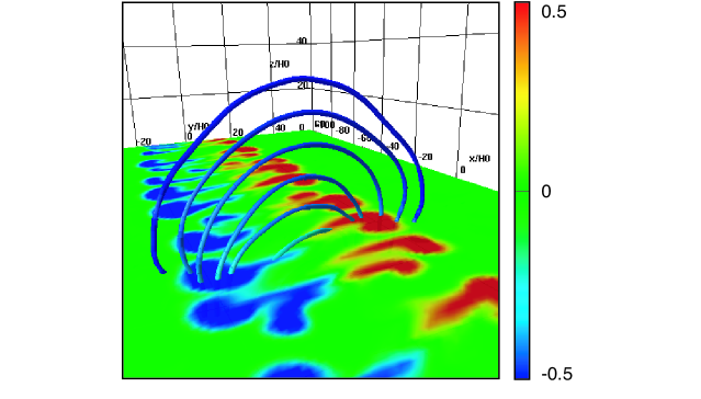
Figure 5: Perspective view of selected field lines that pass through the vertical axis $(x/H_{0},y/H_{0})=(26,0)$ at $t/\tau_{0}=800$, plotted on the photospheric vertical field $B_{z}/B_{0}$.

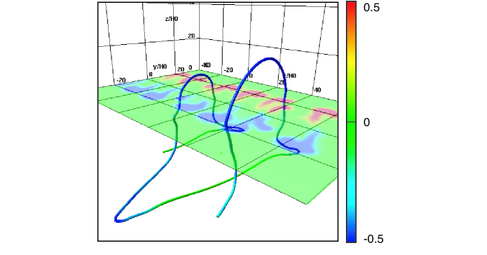
Figure 6: A single field line that connects different photospheric magnetic elements. Plotted is the photospheric vertical field $B_{z}/B_{0}$ at $t/\tau_{0}=800$, which is transparentized.

The tilt of magnetic elements in the central area is caused by the emergence of the inner field lines (kinematic effect). Here, the initial flux tube is uniformly twisted, and thus the pitch angle of inner fields are smaller. Therefore, the footpoints shift as the inner field lines rise. Also, the shearing of two aligned “pores” is due to the Lorentz force acting on the surface field (dynamic effect; see Manchester (2001); Fan (2001)).

4 Summary and Discussion

In this paper, we performed a 3D MHD simulation of the emergence of a twisted flux tube. The initial tube at $-20,000\ {\rm km}$ in the convection zone has a field strength of $2.0\times 10^{4}\ {\rm G}$, a total flux of $6.3\times 10^{20}\ {\rm Mx}$, and a twist of $5.0\times 10^{-4}\ {\rm km}^{-1}$, which starts rising due to its own magnetic buoyancy. On reaching the surface after $t\sim 2.8\ {\rm hr}$, the tube decelerates and extends horizontally ($60\ {\rm Mm}\times 20\ {\rm Mm}$) owing to the convectively stable photosphere ahead of the tube. As the surface field satisfies the criterion for the magnetic buoyancy instability, the field emerges again into the upper atmosphere after $t\sim 4.1\ {\rm hr}$. Eventually, several magnetic domes attain a height of $\sim 7000\ {\rm km}$ at $t\sim 5.6\ {\rm hr}$. The size of the active region grows to $48\ {\rm Mm}\times 12\ {\rm Mm}$, and the photospheric flux amounts to $3.3\times 10^{20}\ {\rm Mx}$. This two-step feature is consistent with our 2D models (papers I and II).

We also observed multiple separation events of the magnetic elements at the photosphere, posterior to the horizontal escaping flow of the compressed plasma. Such separating elements move apart from each other at the rate of $4$–$8\ {\rm km\ s}^{-1}$ and stop at the edges of the active region, which is determined by the extension of the subphotospheric field. The multiple separations are the results of the interchange-mode instability of the rising tube while in the convection zone. The magnetic elements then gather at the edges to make two alignments of the “pores” (tadpole-heads). The alignments show shearing motions at the rate of $\sim 0.5\ {\rm km\ s}^{-1}$, which is explained by the inner field emergence (kinematic effect) and the Lorentz force effect (dynamic effect). Upflows of a few ${\rm km\ s}^{-1}$ and downflows up to $1\ {\rm km\ s}^{-1}$ are observed in the emergent areas and in the cores of surface fields respectively. As far as we know, we have never observed such photospheric features, especially the multiple separations, in previous 3D calculations applying flux tube as an initial condition (e.g. Fan 2001; Archontis et al. 2004). Note that some calculations using flux sheets showed multiple separations via similar instabilities (Isobe et al. 2005; Archontis & Hood 2009).

These features are strongly reminiscent of the observations of NOAA AR 5617 by Strous et al. (1996) and Strous & Zwaan (1999). They found that faculae of both polarities separate from each other toward the edges of the region, which is similar to our findings of multiple separations. Also the shearing motions of the aligned tadpole-heads are consistent with the pores moving along the edges of the region toward the main sunspots. The difference of the tilt of magnetic elements between these two cases is caused by the twist direction. We assumed a right-handed tube in the initial state, which is favorable for the southern hemisphere. AR 5617 appeared in the northern hemisphere, which yields the left-handed twist.

The summary of the comparison between our results and the observations by Strous et al. (1996) and Strous & Zwaan (1999) is presented in Table 1. The size of AR and the velocities are consistent between the two. As for the difference of separation speeds, note that Harvey & Martin (1973) observed that faculae of opposite polarities separate initially at the rate of $>2\ {\rm km\ s}^{-1}$. The photospheric total flux is one digit smaller than the observed value, and we did not find any major sunspots in our active region. These differences may be because, in our calculation, the rising tube stops in 1.4 hours after it appears at the surface. The age of AR 5617 was estimated to be 6.5–7.5 hours old at the beginning of the observation and 8–9 hours old at the end. In the observation, emergence events showed undulatory structures with a typical wavelength of $8\ {\rm Mm}$, while, in our case, each field line does not show undulation at around the surface. Such undulating features might be found in the more resolved calculations or in the calculations including thermal convection (Isobe et al. 2007; Cheung et al. 2010). Strous & Zwaan (1999) summarized their observations as a model in which each emergence event (separation) occurs in a single vertical sheet, which forms a series of sheets aligned in a parallel fashion (see Fig. 8 of their paper). From our results, the separations are explained as the consequence of the interchange-mode instability of the flattened flux tube beneath the surface (see e.g. Fig. 3).

Table 1: Summary of Comparison with AR 5617

	Simulation Results	AR 5617
size of the region	$48\ {\rm Mm}\times 12\ {\rm Mm}$	$50\ {\rm Mm}\times 30\ {\rm Mm}$
vertical unsigned total flux	$3.3\times 10^{20}\ {\rm Mx}$	$4\times 10^{21}\ {\rm Mx}$
age from the appearance	$0$–$1.4\ {\rm hr}$	$6.5$–$9\ {\rm hr}$
separation speed	$4$–$8\ {\rm km\ s}^{-1}$	$0.84\ {\rm km\ s}^{-1}$
shearing speed	$\sim 0.5\ {\rm km\ s}^{-1}$	$0.73\ {\rm km\ s}^{-1}$
upflow velocity	${\rm a\ few\ km\ s}^{-1}$	$0.86\ {\rm km\ s}^{-1}$
downflow velocity	$\lesssim 1\ {\rm km\ s}^{-1}$	$1.26\ {\rm km\ s}^{-1}$
wavelength of emergence pattern	-	$\sim 8\ {\rm Mm}$

On the basis of the numerical results in this paper, we suggest a theoretical picture of the flux emergence and the formation of an active region through the surface, which includes Strous & Zwaan (1999)’s model. Our model is schematically illustrated in Fig. 7. (1) The flux tube rises through the convection zone due to magnetic buoyancy. On approaching the surface, the tube decelerates and becomes flattened because of the photosphere in front of the rising tube. (2) When the photospheric field satisfies the criterion for the magnetic buoyancy instability, further evolution to the corona breaks out. Due to the interchange-mode instability, photospheric magnetogram shows multiple separation events. The separated elements reach the edges of the region, whose size is determined by the subsurface field. These elements then make two alignments of pores. Compare this panel with Fig. 8 of Strous & Zwaan (1999). (3) As the emergence continues, inner fields of the flux tube rise and footpoints shift to show shearing motions. Lorentz force also drives the pores to shear.

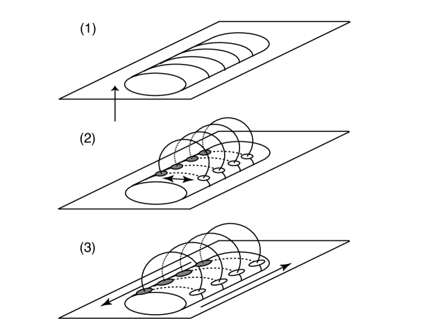
Figure 7: Picture of flux tube emergence and the formation of an active region derived from the calculation results in this paper. Solar surface is indicated by a horizontal slice. (1) Flux tube rising through the convection zone decelerates to form a flat structure beneath the surface. (2) Magnetic elements of opposite polarities are observed to separate due to the interchange-mode instability. White and black ellipses indicate the positive and negative elements. These elements gather at the edges of the active region to make two alignments of pores. (3) Aligned pores show shearing motion when inner fields emerge.

The initial condition of the present experiment ($B_{\rm tube}=67B_{0}=2.0\times 10^{4}G$, $R_{\rm tube}=5H_{0}=1000\ {\rm km}$, and $q=0.1/H_{0}=5.0\times 10^{-4}\ {\rm km}^{-1}$) is the same as that of Case 5 of our 2D cross-sectional calculation in Toriumi & Yokoyama (2011). One of the basic differences between these two simulation results is the rising time from the initial depth of $-20\ {\rm Mm}$ to the surface. In 2D calculation, the flux tube reached the surface in $t\sim 550\tau_{0}=3.8\ {\rm hr}$, while, in 3D case, it took $t\sim 600\tau_{0}=4.2\ {\rm hr}$. That is, the 3D tube rises slower. In 3D case, plasma in the tube apex drains down along the field lines to the both feet of the tube, which drives the tube more buoyant. At the same time, in the 3D regime, the magnetic curvature force pulls down the rising tube. The time difference between the two cases indicates that the curvature force dominates the draining effect in the present 3D experiment.

In the solar interior as well as in the photosphere, several classes of convection may affect the rise of magnetic flux. Recent observations by SOT on board Hinode satellite have revealed the convective nature of the surface field (Lites 2009). Stronger pores ($>1{\rm kG}$) or sunspots, which are not found in this calculation without convection, would be formed through the convective collapse process (Parker 1978). Large-scale upflow supports the rising of the tube, and more flux could be transported to the surface (Fan et al. 2003). Surface convection creates undulating fields, and the cancellation of such fields removes the mass trapped in the U-loop (Isobe et al. 2007; Cheung et al. 2010). This process accelerates the density draining from the surface layer, which may be important to the spot formation. On the other hand, Stein et al. (2011) reported that flux of 20 kG in their convective experiment, the same as used in ours, is too strong, because it produces large, hot, bright granules at the surface, which are not seen in the Sun. This is an interesting difference between the two types of calculations. It should be noted that the initial settings are different in the two cases; we used an initial horizontal flux tube in the convectively stable interior, while, in Stein et al. (2011)’s calculation, uniform horizontal fields are advected into the computational domain by the convective upflows from the bottom boundary. More theoretical and observational studies are needed on the effects of the convection in the whole flux emergence process.