Kinetic cascade beyond magnetohydrodynamics of solar wind turbulence in two-dimensional hybrid simulations

Abstract

The nature of solar wind turbulence in the dissipation range at scales much smaller than the large MHD scales remains under debate. Here a two-dimensional model based on the hybrid code abbreviated as A.I.K.E.F. is presented, which treats massive ions as particles obeying the kinetic Vlasov equation and massless electrons as a neutralizing fluid. Up to a certain wavenumber in the MHD regime, the numerical system is initialized by assuming a superposition of isotropic Alfvén waves with amplitudes that follow the empirically confirmed spectral law of Kolmogorov. Then turbulence develops and energy cascades into the dispersive spectral range, where also dissipative effects occur. Under typical solar wind conditions, weak turbulence develops as a superposition of normal modes in the kinetic regime. Spectral analysis in the direction parallel to the background magnetic field reveals a cascade of left-handed Alfvén/ion-cyclotron waves up to wave vectors where their resonant absorption sets in, as well as a continuing cascade of right-handed fast-mode and whistler waves. Perpendicular to the background field, a broad turbulent spectrum is found to be built up of fluctuations having a strong compressive component. Ion-Bernstein waves seem to be possible normal modes in this propagation direction for lower driving amplitudes. Also signatures of short-scale pressure-balanced structures (very oblique slow-mode waves) are found.

I Introduction

The solar wind is a dilute plasma and known to be in a highly turbulent state Tu and Marsch (1995); Horbury, Forman, and Oughton (2005). It exhibits fluctuations in the electromagnetic field, the plasma density, and bulk flow velocity over a wide range of scalesBruno and Carbone (2005). However, the nature of solar wind turbulence in the intermediate wavenumber regime, situated between the large inertial MHD scales and the small dissipative electron scales, is not well understood. Especially, the role of oblique wave propagation with respect to the background Parker field is currently under debate. Some authors favor a more or less independent behavior of the so called slab component (parallel with respect to the background magnetic field) and 2D turbulence (perpendicular) Montgomery and Turner (1981); Bieber, Wanner, and Matthaeus (1996); Oughton, Matthaeus, and Ghosh (1998). While in this picture the highly oblique 2D-turbulence is believed to be an example of a strongly turbulent plasma state with high-order correlations between the fluctuating quantities, the slab component is assumed to be describable within the framework of weak turbulence theory, i.e. as a superposition of normal modes. Other authors interpret the observed anisotropy as being the result of a kinetic Alfvén wave (KAW) cascade Howes (2008); Schekochihin et al. (2008), which would suggest a preference of fluctuations with $k_{\perp}\gg k_{\parallel}$.

Incompressible, dissipative MHD simulations in two dimensions Shebalin, Matthaeus, and Montgomery (1983) and three dimensions Oughton, Priest, and Matthaeus (1994) show the development of an anisotropy in turbulent spectra with respect to the background magnetic field. In these cases, an initially isotropic spectrum is shown to evolve towards an anisotropic configuration with preferred wavevectors perpendicular to the background field. These authors have shown that the strength of dissipation in the simulations is crucial for the development of anisotropy. The theoretical basis of the geometry in the presence of a strong background field was discussed by Montgomery and Turner Montgomery and Turner (1981) in the framework of a perturbation analysis of the incompressible MHD equations. The resonant conditions $\vec{k}_{1}+\vec{k}_{2}=\vec{k}_{3}$ for the wavevectors and $\omega_{1}+\omega_{2}=\omega_{3}$ for the wave frequencies in a resonant three-wave interaction were found to favor a perpendicular cascade and lead to a suppression of energy transfer in the parallel direction. The strongest turbulent coupling is found to occur if all three frequencies are about zero, a situation which is closest to the hydrodynamic case. This can be completely achieved only if the three-dimensional nature of the solar wind fluctuations is fully resolved, like with a 3-D code that permits to consider both dimensions perpendicular to the background field. However, it was claimed that higher-order couplings could in fact also yield a parallel cascade, yet with a slower growth. These higher-order couplings, the dispersion of the normal modes, and possible compressive effects lead to additional complications in the kinetic regime and make a numerical treatment necessary.

Measurements made by the four Cluster spacecraft have provided further insights into the nature of solar wind turbulence, since multi-spacecraft detections of magnetic fluctuations even permit the analysis of their three-dimensional dispersion properties. However, these measurements support different interpretations. A fully evolved nonlinear turbulent state with a preferred 2D-component beyond the MHD range was found by Alexandrova et al.Alexandrova et al. (2008) The dispersion relation of this mainly perpendicularly structured component might reflect a nonlinear cascade that also occurs at small scales. However, an interpretation on the basis of normal modes, such as the right-handed circularly polarized fast/whistler (F/W) waves, is still possible Narita et al. (2011).

There is strong evidence that the field-parallel component consists at least partly of Alfvén/ion-cyclotron (A/IC) waves, which are dispersive left-hand circularly polarized electromagnetic normal modes of a plasma. The temperature anisotropies and beam structures observed in the solar wind proton distribution functions were explained as resulting from cyclotron-resonant interactions of the ions with these waves Marsch, Ao, and Tu (2004); Heuer and Marsch (2007); Bourouaine, Marsch, and Neubauer (2010). Recently, direct wave measurements have confirmed the existence of A/IC waves in the solar wind Jian et al. (2009). Yet, due to cyclotron-resonant wave-particle interactions, they are strongly damped at wavenumbers corresponding to the inverse inertial length of the resonant ions Ofman et al. (2005), and thus they are not expected to exist at higher wavenumbers. A coexistence of left-handed and right-handed modes has been recently supported by measurements of the angle distribution of the magnetic helicity in the solar wind He et al. (2011). Possible candidates for normal modes beyond the resonant wavenumber range are the F/W modes, which may remain after the dissipation of the A/IC waves Stawicki, Gary, and Li (2001), or an ongoing cascade Howes (2008) of dispersive KAWs. Both these wave modes are right-hand polarized under the conditions prevailing in the solar wind. It is observed that the right-hand polarized waves survive the spectral break, which indicates the transition from the inertial range to the ion dissipative scales, and that they can exist at higher wavenumbers without damping, until the resonant electron scales are finally reached Goldstein, Roberts, and Fitch (1994).

There are other numerical hybrid models available, which treat the kinetic cascade of turbulence beyond the MHD scales. For example Parashar et al.Parashar et al. (2009) achieve an efficient turbulence driving by assuming an Orszag-Tang vortex in the plane perpendicular to the background magnetic field. This configuration leads to perpendicular ion heating, which seems to be not connected to cyclotron-resonant effects. In a later workParashar et al. (2010), the authors also included electron pressure effects and found indications for Bernstein waves. However, the spectrum did not show significant presence of Alfvén or whistler waves but rather a dominance of zero-frequency structures for their geometry and in the strongly turbulent regime. These simulations show that the presence of the electron pressure term in the generalized Ohm’s law can substantially modify the properties of the modeled turbulence. A similar situation has recently been treated in another workMarkovskii and Vasquez (2011) with a special focus on the dissipation of the energy. The formation of intermittent current sheets on short time scales and the related demagnetization of the plasma ions lead to a stochastic heating Chandran et al. (2010).

Our numerical simulation work is focused on studying the transition of isotropic MHD turbulence to non-isotropic kinetic fluctuations on intermediate scales. For this purpose, at least two-dimensional numerical simulations are necessary, by which one can analyze the evolution of turbulence in different directions with respect to the constant background magnetic field. The model system is initialized by a superposition of linear MHD waves. No further external or ongoing driving force is applied, and thus the system will evolve freely from its initial state. Two separate simulation runs are presented, which only differ in the amplitude of the initial perturbation.

II Numerical method

The A.I.K.E.F. code is a numerical hybrid code, which treats ions as particles following the characteristics of the Vlasov equation and electrons as a massless charge-neutralizing fluid. It is based on the work by Bagdonat and MotschmannBagdonat and Motschmann (2002), and its basic properties have later been described extensively by Bagdonat Bagdonat (2005). The code was completely revised, and the possibility for adaptive mesh refinement was included by Müller et al. Müller et al. (2011) The equations of motion for a single proton are

$$\frac{\mathrm{d}\vec{v}_{\mathrm{p}}}{\mathrm{d}t} =\frac{q_{\mathrm{p}}}{m_{\mathrm{p}}}\left(\vec{E}+\frac{1}{c}\vec{v}_{\mathrm{p}}\times\vec{B}\right),$$ (1)

$$\frac{\mathrm{d}\vec{x}_{\mathrm{p}}}{\mathrm{d}t} =\vec{v}_{\mathrm{p}}$$ (2)

for the velocity $\vec{v}_{\mathrm{p}}$ and the spatial location $\vec{x}_{\mathrm{p}}$. The force acting on the particle with charge $q_{\mathrm{p}}$ and mass $m_{\mathrm{p}}$ is the Lorentz force, which is due to the electric field $\vec{E}$ and the magnetic field $\vec{B}$. The speed of light is denoted by $c$. The electron fluid equation of motion delivers the electric field as

$$\vec{E}=-\frac{1}{c}\vec{u}_{\mathrm{e}}\times\vec{B}-\frac{1}{n_{\mathrm{e}}e}\nabla p_{\mathrm{e}},$$ (3)

where the electron bulk velocity is denoted by $\vec{u}_{\mathrm{e}}$, the electron number density by $n_{\mathrm{e}}$, the elemental charge by $e$, and the electron fluid pressure by $p_{\mathrm{e}}$. The electrons are assumed to be isothermal, and thus the pressure depends on the electron number density according to $p_{\mathrm{e}}\propto n_{\mathrm{e}}$. Quasi-neutrality requires that $n_{\mathrm{p}}=n_{\mathrm{e}}$. The proton density and the proton bulk velocity $\vec{u}_{\mathrm{p}}$ are obtained as the first two moments of the proton distribution function at every step in time.

The magnetic field is obtained from the induction equation following from Faraday’s law:

$$\frac{\partial\vec{B}}{\partial t}=\nabla\times\left(\vec{u}_{\mathrm{p}}\times\vec{B}\right)-\nabla\times\left(\frac{c}{4\pi\varrho_{\mathrm{c}}}\nabla\times\vec{B}\times\vec{B}\right).$$ (4)

The ion charge density $\varrho_{\mathrm{c}}$ corresponds to the proton number density calculated as the zeroth velocity moment of the distribution function of all protons.

The boundaries of the simulation box are set to be periodic, and the particles are initialized with a Maxwellian velocity distribution that is shifted to the given values for the initial bulk velocities. The width of the Maxwellian distribution is determined by the respective species’ plasma beta, which represents the ratio of the ion thermal to the magnetic energy density. The beta is set to $\beta_{\mathrm{p}}=0.05$ for the protons. The electron beta is fixed at $\beta_{\mathrm{e}}=0.5$. In this beta regime, even low amplitudes of magnetic fluctuations will have a strong influence on the motion of the particles due to their high magnetization. All spatial length scales are normalized and given in units of the proton inertial length, $\ell_{\mathrm{p}}=c/\omega_{\mathrm{p}}$, with the proton plasma frequency $\omega_{\mathrm{p}}=\sqrt{4\pi n_{\mathrm{p}}q_{\mathrm{p}}^{2}/m_{\mathrm{p}}}$. All time scales are in units of the inverse proton gyro-frequency $\Omega_{\mathrm{p}}=q_{\mathrm{p}}B/(m_{\mathrm{p}}c)$. In these units, the two-dimensional integration box has a size of $250\times 250$, which is covered by $1024\times 1024$ cells, each of which filled with 500 superparticles representing the real number density of the protons. In this spatial configuration, one grid step corresponds to about $0.24\ell_{\mathrm{p}}$ in the calculation. The data is recorded with a grid resolution of $\Delta x=0.5\ell_{\mathrm{p}}$ to keep the amount of data reasonable. This corresponds to a maximum resolvable wavenumber of $\ell_{\mathrm{p}}k_{\mathrm{res}}\approx\pi/0.5\approx 6.3$, which is adequate for an appropriate coverage of the transition from MHD into the kinetic regime. For all vector quantities, three components are evaluated. Approaches of this form are sometimes referred to as 2.5D simulations. A divergence-cleaning algorithm is applied to guarantee numerical stability.

The initial magnetic field is given as a superposition of linear Alfvén waves according to

$$\delta B_{x}=\sum\limits_{m=1}^{m_{\max}}\sum\limits_{n=1}^{n_{\max}}b_{n}\cos(k_{n}y\sin\vartheta_{m}+k_{n}z\cos\vartheta_{m}+p_{n,m}),$$ (5)

where the constant background field $\vec{B}_{0}$ is aligned along the $z$-axis. A random phase shift $p_{n,m}$ is applied to each wave. The amplitudes $b_{n}$ are fixed in such a way that the power spectrum follows a Kolmogorov power lawKolmogorov (1941) in wavenumber with the scaling $\propto k^{-5/3}$. The total power of the composed wave field is made equal to the power of a monochromatic wave with $\delta B=0.01B_{0}$ for Run A and to $\delta B=0.1B_{0}$ for Run B. The first value corresponds to a situation with a weaker turbulence level or a higher background field as prevailing in the solar corona, while the second value represents realistic solar wind conditions. The angles $\vartheta_{m}$ cover $360^{\circ}$ of propagation directions by $m_{\max}=50$ discrete values, and the spectrum ranging between $k_{0}=0.05$ and $k_{\max}=0.2$ is covered by $n_{\max}=20$ waves. The upper limit $k_{\max}$ is quite high compared to typical MHD scales but, still, in the dispersion-less range in first order. The initial velocity is obtained from the Alfvénic polarization relation

$$\frac{\delta\vec{V}}{V_{\mathrm{A}}}=\mp\frac{\delta\vec{B}}{B_{0}}$$ (6)

with the Alfvén speed $V_{\mathrm{A}}=\ell_{\mathrm{p}}/\Omega_{\mathrm{p}}$.

III Results

In this section some results of the numerical simulation runs are shown. We ran the code for a sufficiently long time so that an evolved nonlinear dynamic plasma state could be expected. This was typically the case after an evolution time of about 500 gyro-periods, at which time the system was analyzed.

III.1 Results for simulation Run A

For the analysis of the results from Run A, Fourier transformations in two dimensions were applied subsequently to the magnetic field data and the density data. The power spectral density was then calculated, and could be shown to depend on the wavenumbers $k_{z}$ for the direction parallel to the background field and $k_{y}$ perpendicular to it. The resulting magnetic field power spectral density is shown in Fig. 1, and the power spectral density of the compressive fluctuations is shown in Fig. 2.

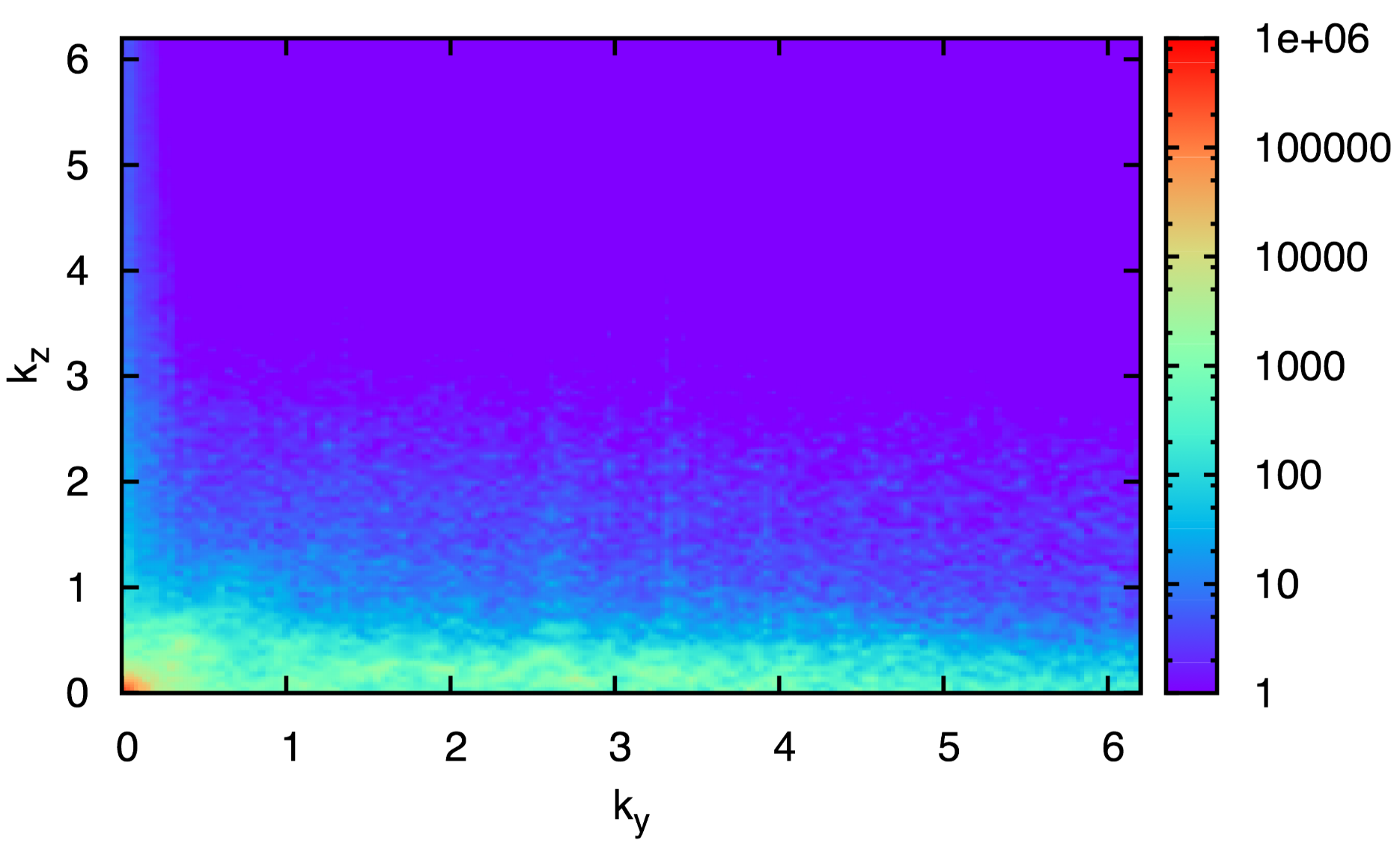
Figure 1: Two-dimensional power spectral density of magnetic field fluctuations in arbitrary units for Run A. The background magnetic field is oriented along the $k_{z}$-axis. The cascade of energy to higher wavenumbers occurs preferentially in perpendicular direction.

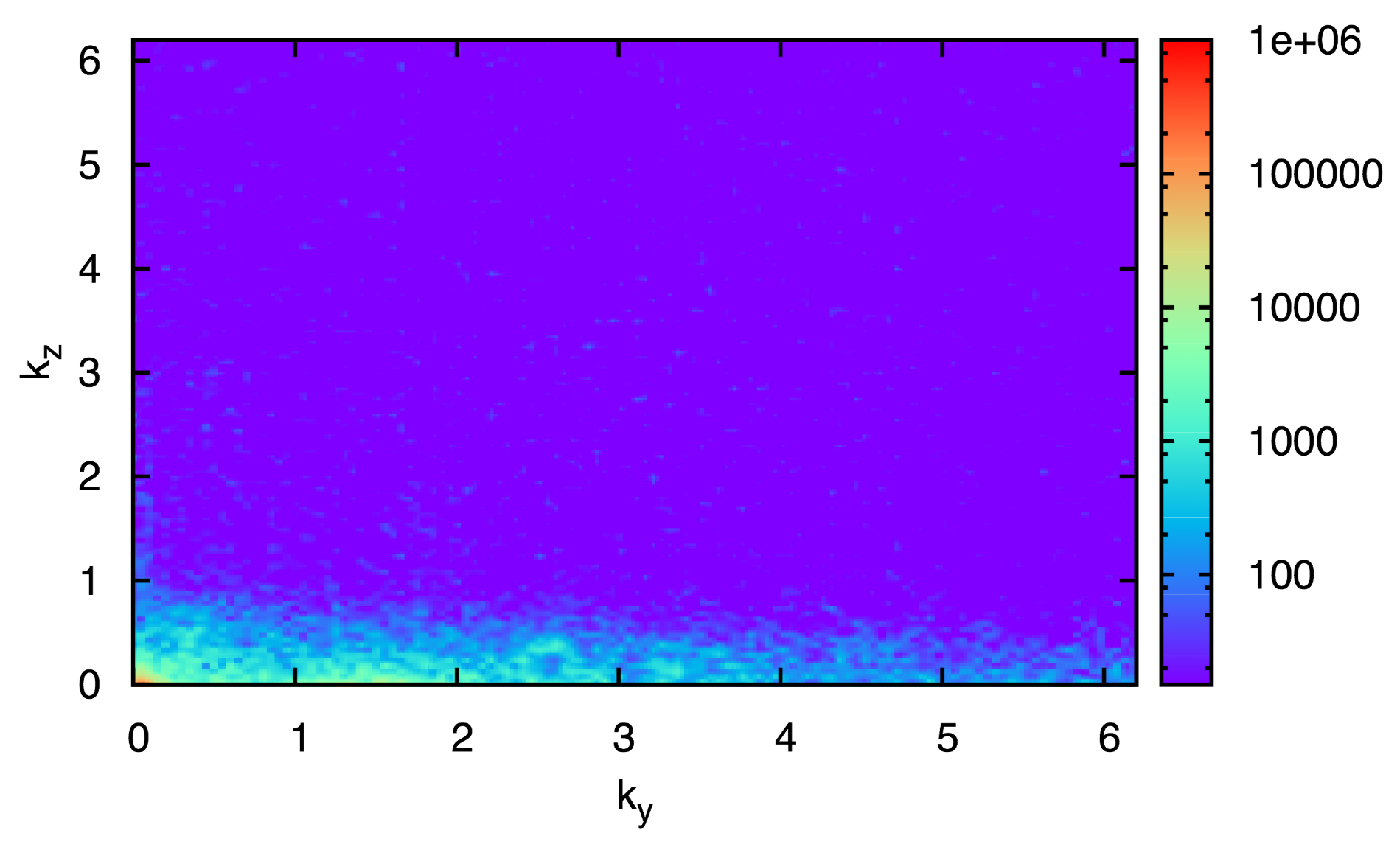
Figure 2: Power spectral density of compressive fluctuations in the proton number density in arbitrary units for Run A. The spatial variation of the fluctuations occurs mainly perpendicular to the background magnetic field.

Apparently, the magnetic field fluctuations show a preferred alignment with the direction perpendicular to the background magnetic field. Especially, turbulence energy is spreading in this direction to much higher wavenumbers than in the parallel direction. But also the parallel fluctuations at wavenumbers beyond the initialized range are excited and gain energy. The compressive density fluctuations, however, are mainly aligned perpendicular to the background field and have almost no components parallel to $\vec{B}_{0}$.

Cuts through the two-dimensional spectra along the perpendicular direction are shown in Fig. 3.

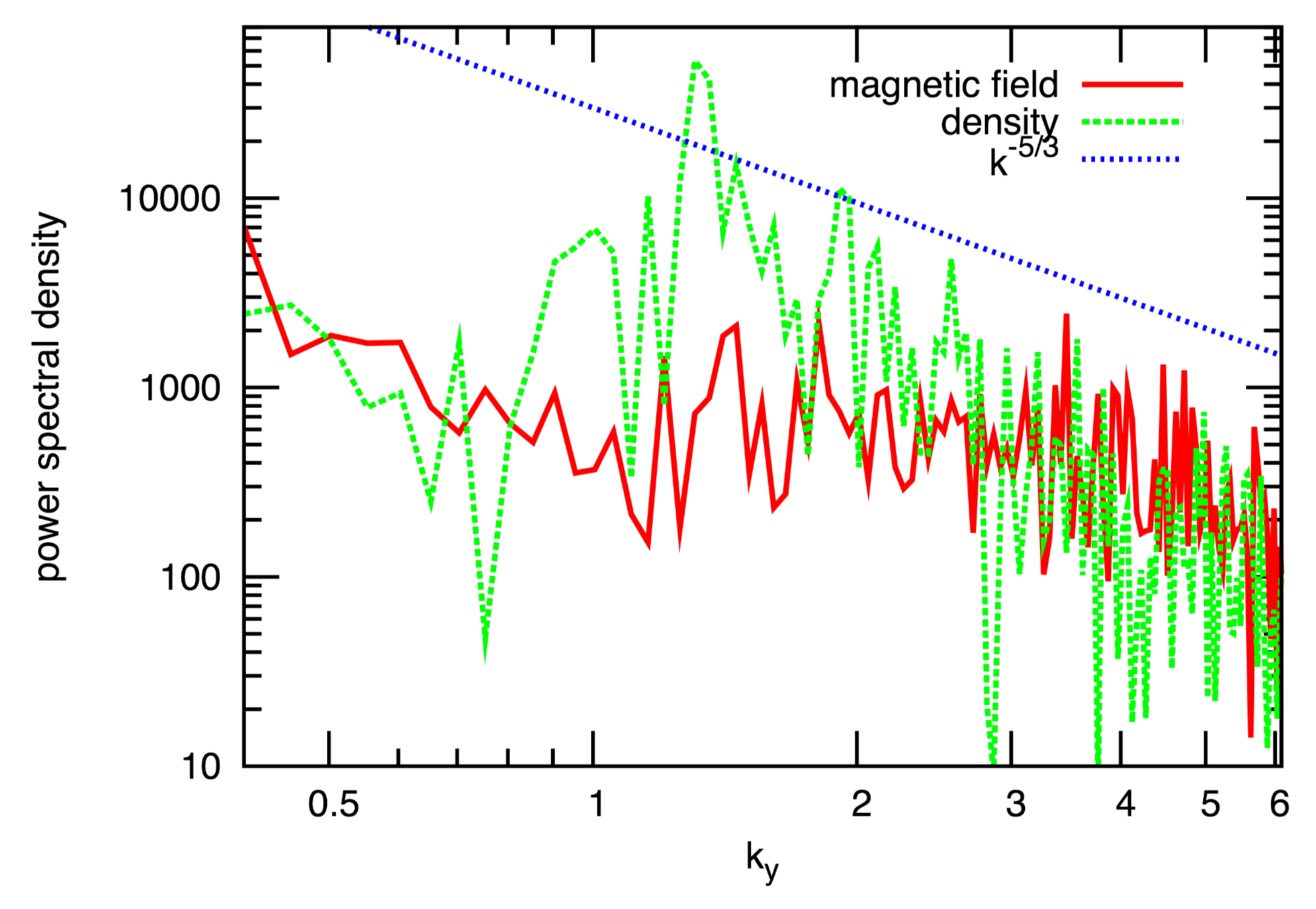
Figure 3: Power spectral density of fluctuations in the magnetic field and density at $t=500$ along the perpendicular direction for Run A. A power law with spectral index $-5/3$ is shown additionally, in order to estimate the slope of the spectrum.

The power spectral density of the compressive fluctuations in the proton number density is enhanced for $k_{y}\gtrsim 1$ and follows mainly a power law with a slightly steeper index than $k^{-5/3}$ in this range. The magnetic field spectrum is flatter in the dispersive range.

To study the nature of these fluctuations Fourier transformation can also be used, but here is applied in the time domain leading to the corresponding dispersion diagrams. Therefore, first the two-dimensional spatial Fourier transformation is applied, and the result is taken in one dimension only (parallel or perpendicular to $\vec{B}_{0}$), and then the data are again Fourier transformed yet in time. The result for the parallel magnetic field dispersion is shown in Fig. 4.

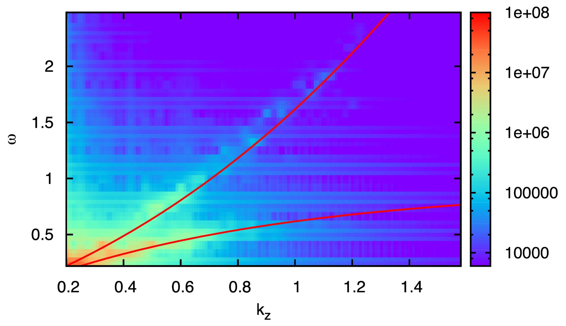
Figure 4: Dispersion relation of magnetic field fluctuations parallel to the background magnetic field at $t\approx 500$ for Run A. The overplotted red lines indicate the F/W (upper line) and A/IC (lower line) wave branches calculated directly from the cold-plasma dispersion relation.

Most of the power is found at low wavenumbers and low frequencies and still close to the initial distribution of the waves. Spreading of power at low parallel wavenumbers with low frequencies is an indication for ongoing MHD turbulence. Two sharp branches can clearly be seen beyond the initial wavenumber limit at $k_{\max}=0.2$. For an easier identification of them, the cold-plasma dispersions for the left-handed A/IC waves and for the right-handed F/W waves are additionally shown in the parallel dispersion diagramStix (1992). The observed parallel dispersion agrees well with that of the linear normal modes. The A/IC branch ends at a wavenumber value below $1$, whereas the right-handed branch continues to higher wavenumbers and frequencies.

The perpendicular magnetic field dispersion is depicted in Fig. 5. Since the density fluctuations are mainly perpendicularly oriented, their parallel dispersion diagram is not shown here. But the perpendicular dispersion diagram is illustrated in Fig. 6.

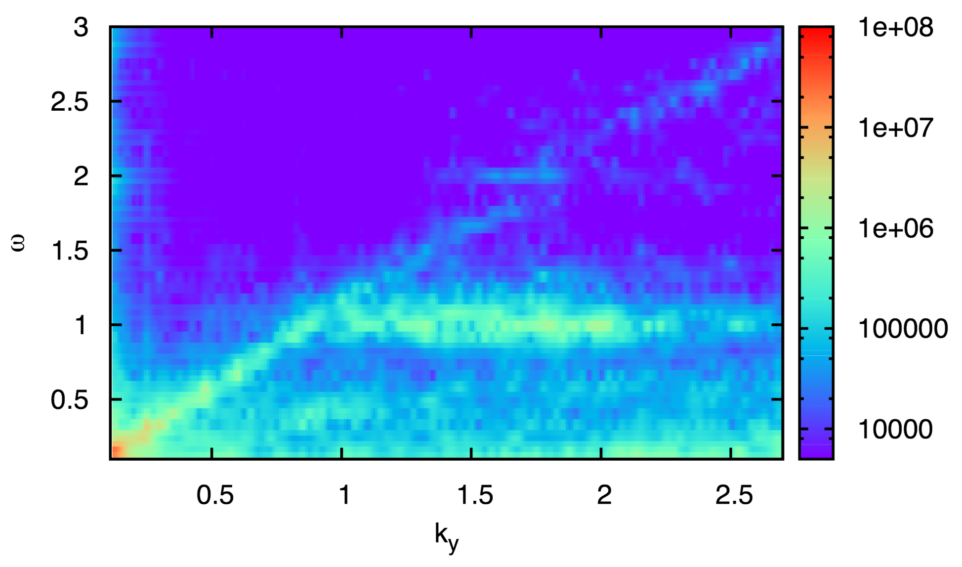
Figure 5: Dispersion relation of magnetic field fluctuations perpendicular to the background magnetic field at $t\approx 500$ for Run A.

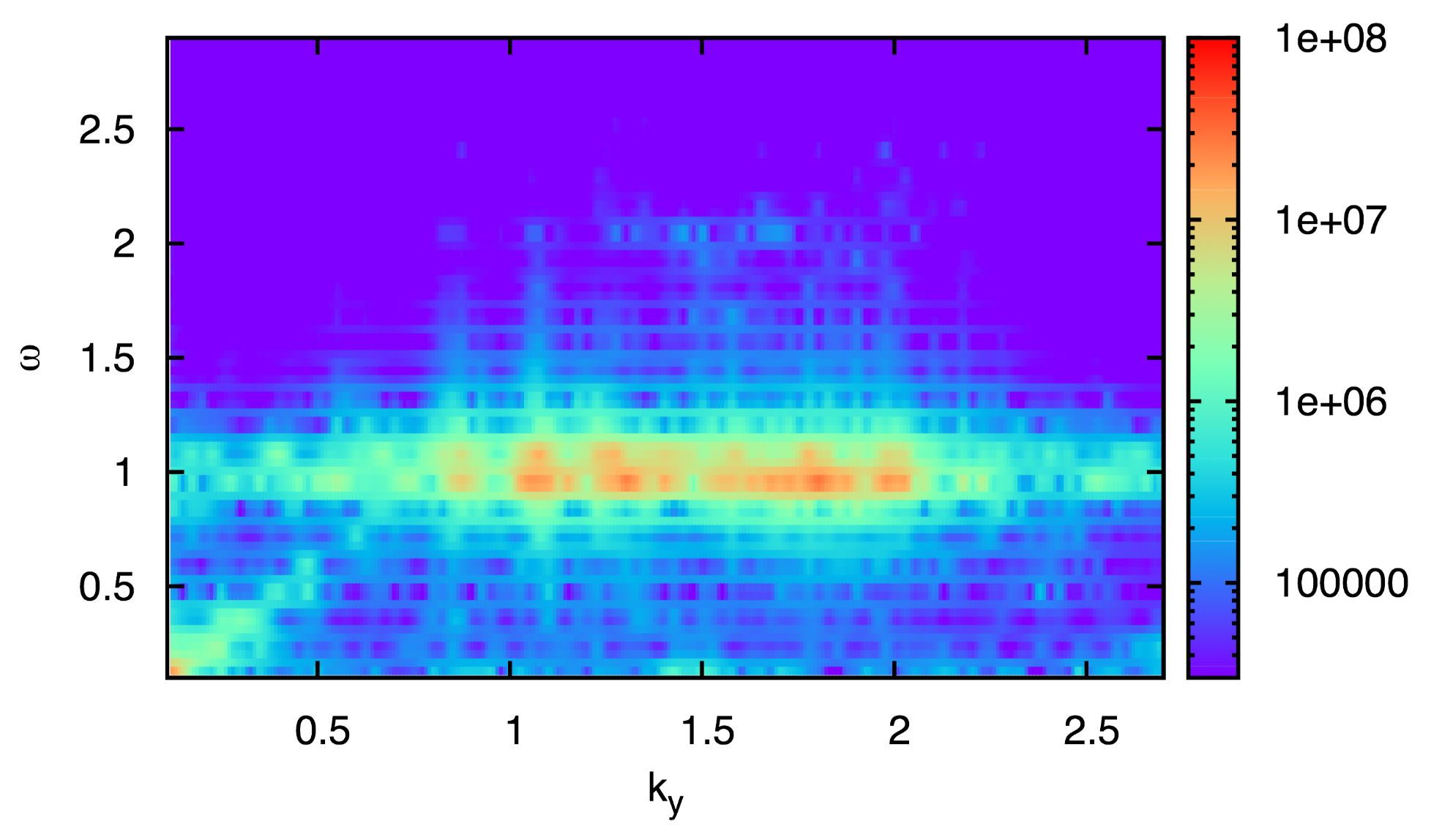
Figure 6: Dispersion relation of density fluctuations perpendicular to the background magnetic field at $t\approx 500$ for Run A. The fluctuations coincide well with the magnetic fluctuations.

These two dispersion diagrams show a common structure in the fluctuations in the form of a band signature of the intensity near the gyro-frequency and at higher harmonics in the magnetic and compressive dispersion. We believe that this is a typical indication for the occurrence of ion-Bernstein wavesStix (1992); Brambilla (1998); Swanson (2003). A linear branch with weak power is observed at $\omega/k=1$ in the perpendicular dispersion plots of the magnetic field and density fluctuations. It corresponds to the linear fast-mode wave in a low-beta plasma. A linear Alfvén wave does not propagate perpendicular to the background magnetic field, and therefore can be excluded from the interpretation of this branch. A coupling between it and the ion-Bernstein modes is not observed, and may presumably not be detectable given the spectral resolution of the numerical analysis applied.

There is further power distributed in compressive and magnetic structures at $\omega\approx 0$. These signatures cannot be explained as ion-Bernstein waves, because they do not have the minimum frequency of $\Omega_{\mathrm{p}}$ and are merely spatial structures constant over time. To analyze their nature, the possible correlation between the magnetic pressure $P_{B}=\delta\vec{B}^{2}/(8\pi)$ and the density fluctuations $\delta n$ can be applied. It is defined as

$$C\equiv\frac{\langle\delta n\,\delta|\vec{B}|^{2}\rangle}{\sqrt{\langle\delta n^{2}\rangle\langle\delta|\vec{B}|^{4}\rangle}},$$ (7)

where the brackets indicate a certain way of averaging. This averaging is here done only perpendicular to the magnetic field and in the time domain. Averaging over a long time scale corresponds to structures with low frequency and averaging over short time scales corresponds to higher frequencies. The same is true in the spatial domain.

The result of this calculation is shown in Fig. 7.

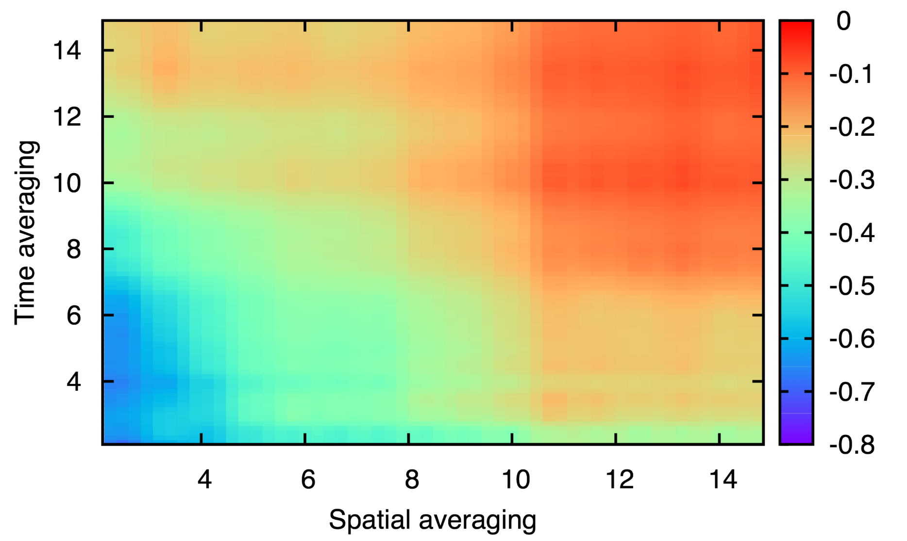
Figure 7: Correlation coefficient $C$ between fluctuations of magnetic pressure and density depending on the averaging in space and time for Run A. A strong anti-correlation is found up to long averaging times, which correspond to low frequencies in the dispersion diagrams. This is an indication for the existence of PBSs. The units are given in the above introduced normalization.

At high values for the time averaging and at low values for the spatial averaging, a strong anti-correlation between $\delta P_{B}$ and $\delta n$ is found. This indicates the existence of pressure-balanced structures (PBSs), which correspond to steepened-up slow-mode waves in the perpendicular direction Tu and Marsch (1994). They are characterized by their direction of propagation and the strong anti-correlation between $\delta P_{B}$ and $\delta n$. The classical slow-mode wave does not propagate at 90 degrees, but in this direction transforms into a tangential discontinuity, which some of the numerical structures may represent. Therefore, it seems useful to analyze the perpendicular correlation only, since a parallel slow-mode component is not expected to survive but to undergo strong Landau damping. However, it is also important to state that our simulation results cannot be unequivocal on this issue, because at other positions and different time intervals the anti-correlation is not always pronounced, and some cases even show a positive correlation. These findings should be understood just as an indication for the presence of PBSs. In this special case, the correlation remains positive for only a few averaging steps in time.

The temperature of the treated protons stays mainly constant in this case. Also a potential temperature anisotropy is not observed.

III.2 Results for simulation Run B

Run B with a higher initial amplitude is in general consistent with the previously discussed Run A. Therefore, we limit our description to the major similarities and differences between the two runs. The magnetic field spectrum is shown in Fig. 8.

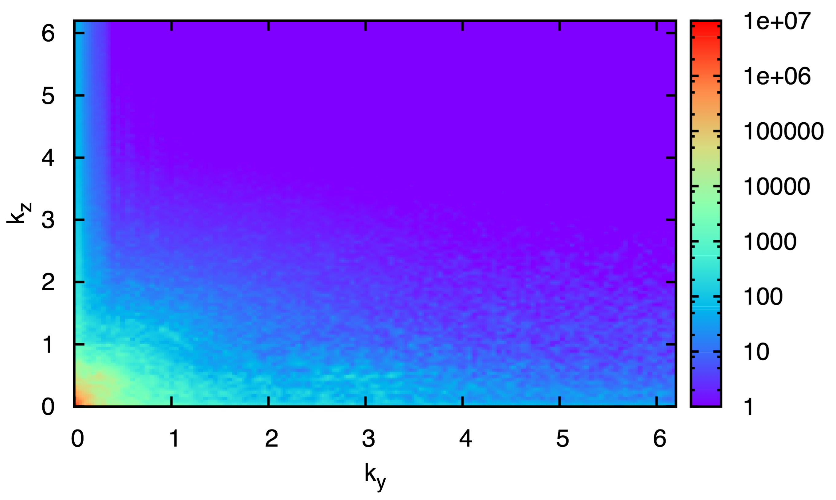
Figure 8: Two-dimensional power spectral density of magnetic field fluctuations in arbitrary units for Run B. The background magnetic field is oriented along the $k_{z}$-axis. Also in this case, the cascade is preferentially perpendicular.

The cascade is also preferentially oriented in the perpendicular direction. However, a larger wavenumber range is filled isotropically around $\vec{k}=0$. The compressive component is also very similar to the one in Run A (not shown here).

A cut along the perpendicular direction in the power spectra for the magnetic field and density fluctuations is shown in Fig. 9.

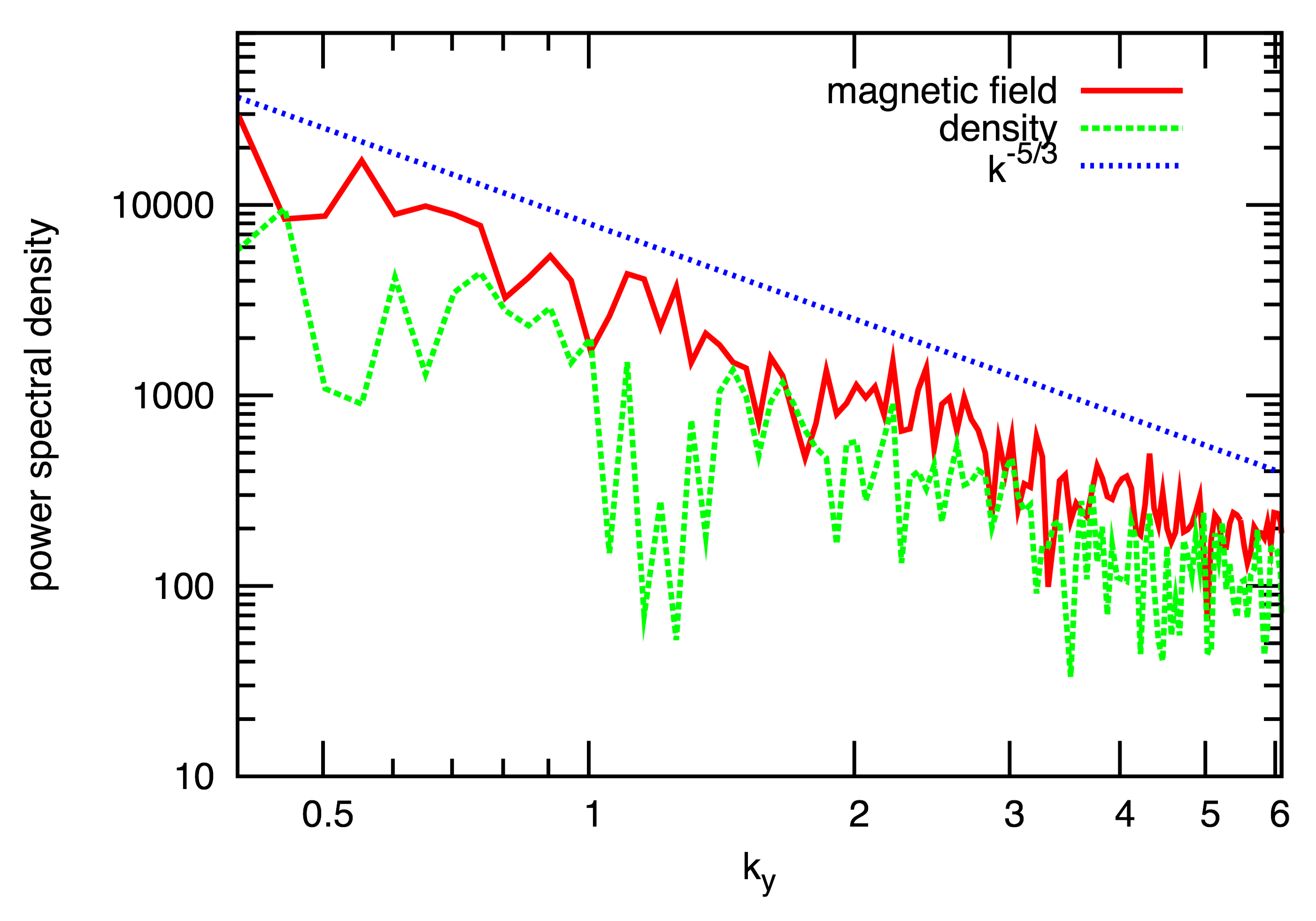
Figure 9: Power spectral density of fluctuations in the magnetic field and density at $t=500$ along the perpendicular direction for Run B.

In this case, the spectrum follows more closely a slope with the power index of $-5/3$.

The dispersion analysis of the parallel fluctuations is shown in Fig. 10 and reveals also the same normal mode structure as in Run A, yet with a stronger intensity.

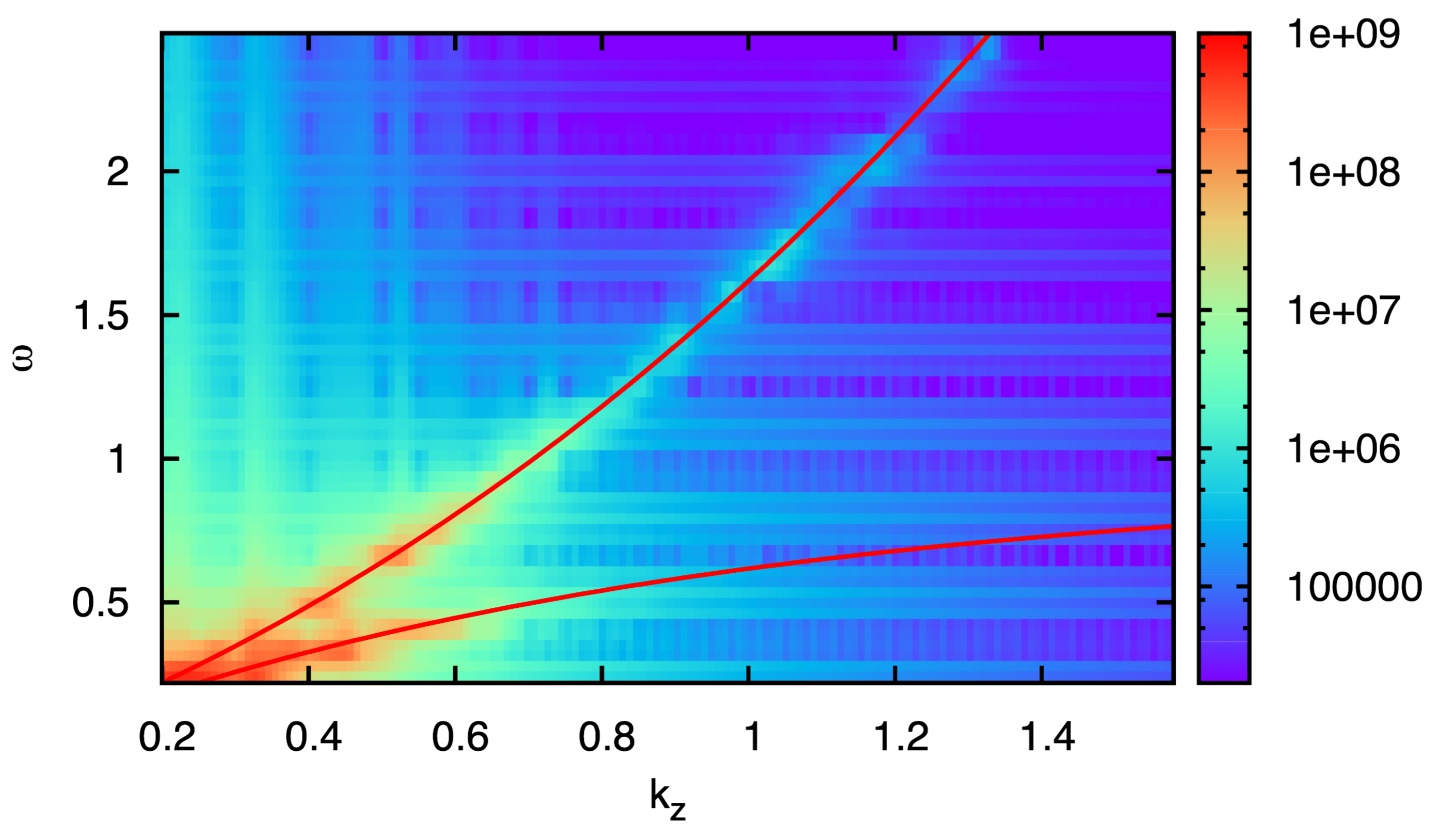
Figure 10: Dispersion relation of magnetic field fluctuations parallel to the background magnetic field at $t\approx 500$ for Run B. The overplotted red lines indicate again the theoretical cold-plasma dispersion relations.

A substantial difference occurs in the perpendicular dispersion, which is shown in Fig. 11.

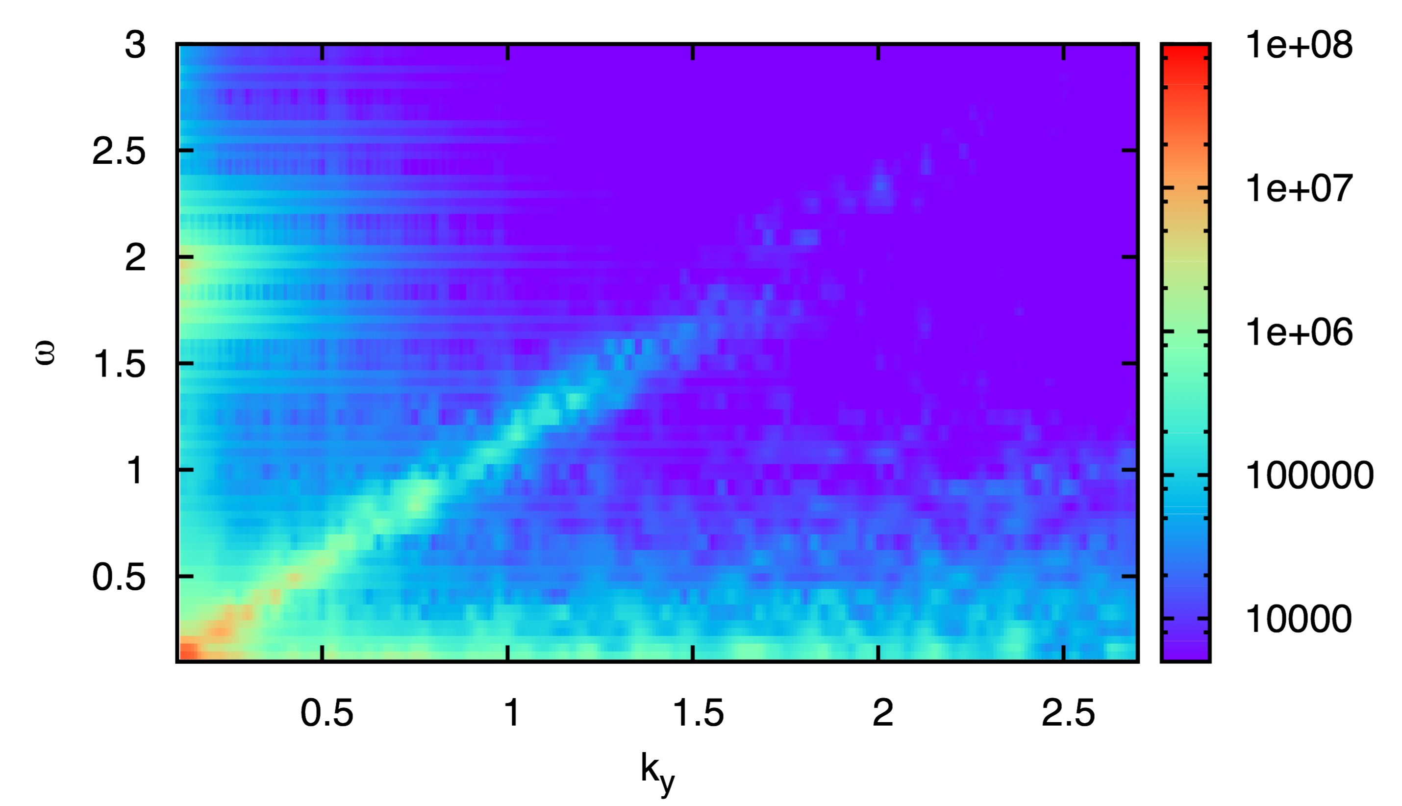
Figure 11: Dispersion relation of magnetic field fluctuations perpendicular to the background magnetic field at $t\approx 500$ for Run B.

The ion-Bernstein signatures, which have been observed in Run A, are not any longer visible in this dispersion diagram and are also not present in the compressive dispersion (not shown here). Instead, the perpendicular fast mode is more pronounced.

The low-frequency part also shows an anti-correlation between $\delta P_{B}$ and $\delta n$ under certain conditions and, therefore, seems to represent the same structures as observed in Run A.

While the wave power in the low-amplitude case was too low to produce significant proton heating, this situation changed in the case of Run B. The temperature evolution of the protons is shown in Fig. 12.

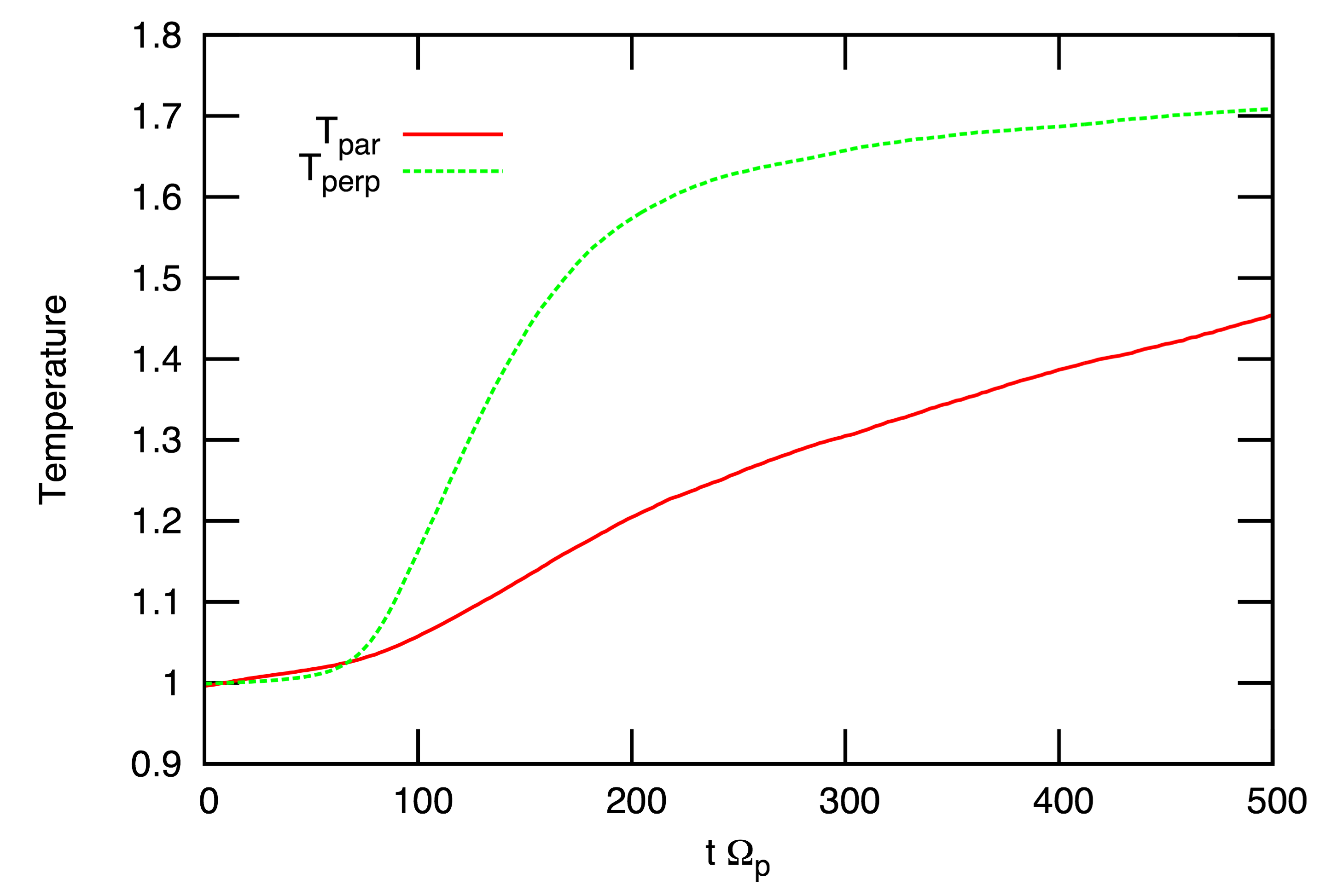
Figure 12: Temperature evolution of the protons for Run B. The temperatures versus time in the parallel and perpendicular direction with respect to the background magnetic field are shown. They are normalized to their initial values.

Their temperatures increase, and a temperature anisotropy with higher perpendicular than parallel temperature with respect to the background magnetic field is found. The perpendicular temperature raises faster than the parallel one and reaches a saturation value of about 1.7 of the initial perpendicular temperature.

IV Discussion and Conclusions

According to our numerical simulations, the turbulent energy cascades preferentially into the direction perpendicular to the background magnetic field, which is consistent with the recent results of other numerical simulationsMacBride, Smith, and Forman (2008); Jiang, Liu, and Petrosian (2009); Markovskii, Vasquez, and Chandran (2010) and space observations Chen et al. (2010); Sahraoui et al. (2010); Narita et al. (2011). However, there is also a parallel cascade present, and the nature of all the relevant fluctuations shall now be discussed in dependence upon the direction of propagation.

The parallel fluctuations seem to be well described as a superposition of normal modes. In the range above the ion-cyclotron scales they are mainly F/W waves, as it has been suggested before by many authors Matthaeus, Goldstein, and Roberts (1990); Stawicki, Gary, and Li (2001); Gary, Saito, and Li (2008). This finding is in agreement with observations in the solar wind indicating that left- and right-handed normal modes coexist until a wavelength of the order of $1/\ell_{\mathrm{p}}$, where the left-handed waves undergo resonant wave-particle interactionsGoldstein, Roberts, and Fitch (1994) with cyclotron absorption. At higher wavenumbers, only right-handed waves can survive the transition into the intermediate dissipative range of solar wind turbulence He et al. (2011). Linear wave damping seems to dominate the dissipation compared to nonlinear damping effects, as it has been discussed before in the context of interstellar medium heatingSpangler (1991).

Parallel A/IC waves are the most prominent of the left-handed waves that are known to undergo strong ion-cyclotron damping under certain conditions Marsch (2006). The observed perpendicular solar wind heating Marsch, Ao, and Tu (2004) can, thus, be largely explained by absorption of this left-handed normal mode, which is mostly observed in parallel propagation. This is most probably also the explanation for the establishment of the observed temperature anisotropy in the simulation Run B with the higher initial amplitude. Quasi-perpendicular ion-Bernstein waves may also be able to heat the plasma due to cyclotron-resonance effects. Therefore, also the here identified ion-Bernstein modes could provide a heat source for the ions. The efficiency of the dissipation of ion-Bernstein waves strongly depends on beta and is higher for larger beta values. This effect is also discussed by Markovskii et al. Markovskii, Vasquez, and Chandran (2010) in the context of a cascade of F/W waves. This may be a possible explanation for the vanishing of the ion-Bernstein modes in Run B because the temperature increase due to the resonant heating corresponds to a change in the plasma beta.

The reason for the flatter power index in Fig. 3 compared to the Kolmogorov scaling, which is instead found in Run B as seen in Fig. 9, may be that in the Run A with lower initial stirring amplitude the cascade develops more slowly, and the turbulence is not yet fully evolved at the applied integration time.

Fast waves themselves can of course also be dissipated by ions if they propagate obliquely Marsch (2006). This effect may, however, be slow when compared to the cyclotron-resonant absorption of A/IC waves and needs to be accumulated over a longer solar wind travel time to become significant. The intensity of the ion-Bernstein bands is more pronounced for higher electron betas, which is an indication for the electrostatic character of these wave structures. A kinetic micro-instability, which is able to excite ion-Bernstein waves in a way consistent with the wave structures observed in magnetospheres, has recently been treated in detail with particle-in-cell simulationsLiu, Gary, and Winske (2011).

The nature of the perpendicular low-frequency fluctuations cannot be uniquely identified. There is evidence for the existence of pressure-balanced structures (PBSs), which show the typical anti-correlation between $\delta P_{B}$ and $\delta n$. It is observed in the solar wind that this anti-correlation dominates on shorter time averagingTu and Marsch (1995). A positive correlation dominates on longer time-scales, which is interpreted as the indication for co-rotating interaction regions as a result of interactions between different solar wind streams with high and low outflow speeds. The correlation shows a typical spatial dependence on large scales in the solar wind. A positive correlation is built up inside 0.7 to 0.8 AU, whereas the anti-correlation is already observed closer to the Sun prevailing over a large distance range Roberts et al. (1987). Cluster observations also show PBSs on smaller scales than the typical low-frequency MHD rangeYao et al. (2011). The origin of these structures, however, is unclear. Part of these structures may be generated by a nonlinear cascade of the turbulence into the intermediate wavenumber range, as it is revealed by the simulations. Other possible non-propagating perpendicular wave structures are mirror modes or Weibel modes.

The predominance of an anti-correlation in $\delta P_{B}$ and $\delta n$ at some positions supports the interpretation of these structures in terms of PBSs. But they are of dynamic nature and a minor component driven by the perpendicular incompressible fluctuations which are the major component and represent the key nonlinearly interacting degrees of freedom. Therefore, incompressible turbulence prevails, but additionally the compressive PBS-like correlations occur at the same time. The interpretation of such fluctuations in terms of static PBSs would be closer to a normal-mode picture of the modeled fluctuations but perhaps not quite adequate. However, the present simulation results do not permit a definite conclusion on the nature of the weakly compressive fluctuations.

In a recent model Howes, TenBarge, and Dorland (2011), the transition from strong to weak turbulence at small scales is discussed. The authors assume a completely suppressed parallel cascade for the kinetic Alfvén waves considered in their model, deduced from the suppressed parallel cascade of weak turbulence in the incompressible MHD limit. According to their model, the anisotropy in the strongly turbulent domain is expected to follow the phenomenology of critically balanced turbulence, which is not applicable to weak turbulence. Our simulation shows, however, that the parallel cascade is not fully suppressed, even not in the limit of weak turbulence. Yet, the spectral transfer is clearly anisotropic and shows a preference for the perpendicular cascade.

The MHD modes with low wavenumbers mainly keep their amplitude level during their temporal evolution and stay mostly isotropic. A longer integration time might also show a preferred direction of the cascade at lower wavenumbers, as it was observed by other authorsWicks et al. (2010). Waves with higher wavenumbers, however, may hand over their energy more easily. This underlines that the spectral transfer occurs also in this case locally in wavenumber space, as it seems typical for a turbulent cascade Coleman (1968). This effect is also incorporated in models concerning the coronal heating problem, where a nonlinear local cascade is often effectively described as an advection and diffusion process in wavenumber spaceZhou and Matthaeus (1990); Cranmer and van Ballegooijen (2003).

Normal modes can also be directly excited from the ubiquitous thermal fluctuations in a plasma Araneda, Astudillo, and Marsch (2011). However, their amplitudes usually stay on a very low level, and they do not increase with time at the expense of energy drawn from lower wavenumbers, as it is observed in our simulations. Therefore, it is reasonable to interpret the observed wave structures at higher frequencies as being the products of processes driven from the low-frequency side in the sense of a nonlinear mechanism, instead of being of purely thermal origin with a typical energy content of the order $k_{\mathrm{B}}T$.

If the wave power in the inertial range is much higher than assumed here, other nonlinear couplings might play a role also in the kinetic regime. This can possibly destroy the normal mode superposition even above $k=1$, and then lead to a completely different picture with respect to both the spectral transfer to higher wavenumbers and the dispersion structure in the dispersive spectral range.

Parashar et al.Parashar et al. (2011) have shown that the properties of the turbulence driver are very important for the generation and the further evolution of plasma turbulence. The dependence on the driving frequency is crucial in the context of AC coronal heating models, since footpoint motions on different timescales are expected to be the main source for the turbulence, which is then assumed to heat the coronal plasma in these models.

Finally, our simulation box is small compared to all global structures in the solar wind, and the numerical conditions are, hence, homogeneous in the above considerations. There are, however, recent indications that inhomogeneities foster the thermalization of wave energy Ofman, Viñas, and Moya (2011). This effect may play also a role for the global evolution of the solar wind.