TRANSPORT VIA CLASSICAL PERCOLATION AT QUANTUM HALL PLATEAU TRANSITIONS

Abstract

We consider transport properties of disordered two-dimensional electron gases under high perpendicular magnetic field, focusing in particular on the peak longitudinal conductivity $\sigma_{xx}^{\mathrm{peak}}$ at the quantum Hall plateau transition. We use a local conductivity model, valid at temperatures high enough such that quantum tunneling is suppressed, taking into account the random drift motion of the electrons in the disordered potential landscape and inelastic processes provided by electron-phonon scattering. A diagrammatic solution of this problem is proposed, which leads to a rich interplay of conduction mechanisms, where classical percolation effects play a prominent role. The scaling function for $\sigma_{xx}^{\mathrm{peak}}$ is derived in the high temperature limit, which can be used to extract universal critical exponents of classical percolation from experimental data.

PACS numbers: 73.43.Qt, 64.60.ah, 71.23.An

1 Introduction

The quantum Hall effect[1, 2] in two-dimensional electron gases (2DEG) follows from a disorder-induced localization process peculiar to the situation of large perpendicular magnetic fields $B$. While the formation of discrete Landau levels (LL) at energies $E_{n}=\hbar\omega_{c}\left(n+\frac{1}{2}\right)$ can account for the existence of robust quantum numbers (with $\omega_{c}=|e|B/m^{\star}$ the cyclotron frequency, $e=-|e|$ the electron charge, $m^{\star}$ the effective mass, $\hbar$ Planck’s constant divided by $2\pi$, and $n$ a positive integer), the existence of a macroscopic number of localized states in the bulk of 2DEG is an essential aspect of quantum Hall physics[3]. Many questions are yet still open thirty years after the initial discovery: i) for metrological purposes[4], which physical processes are limiting the plateau quantization of the Hall conductivity near the universal value $\sigma_{xy}=ne^{2}/h$?; ii) what is the nature of the localization/delocalization transition from one plateau to the next[5, 6, 7], whereupon highly dissipative transport sets in? Theoretically, the problem in its full complexity requires to understand the quantum dynamics of electrons subject to the Lorentz force and random local electric fields, possibly with the inclusion of dissipative processes such as electron-electron and electron-phonon interaction, that are sensitive issues when one considers transport properties.

So far, a lot of attention was turned towards the understanding of the delocalization process in terms of a zero-temperature quantum percolation phase transition, which still remains a challenge for the theory[5, 6, 7], despite intriguing experimental evidence from transport[8, 9] and local scanning tunneling spectroscopy[10]. In this framework, the quantum tunneling and interference of the guiding center trajectories within a complex percolation cluster allow dissipation to develop in a non-trivial way at the quantum Hall transition. Obviously, increasing temperature from absolute zero will generate inelastic processes limiting the coherence between saddle points of the disorder lanscape, so that the quantum character of the transition becomes progressively irrelevant. In that case, a simpler quasiclassical transport theory becomes valid[11, 12, 13, 14], which incorporates the fast cyclotron motion with the slow guiding center drifting, and takes into account inelastic contributions to transport. The transport problem does not become however totally trivial, because classical percolation in the related advection-diffusion regime is still not fully understood[15].

The aim of the present paper is two-fold. First, we will show in Sec. 2 that high mobility samples display a very rich temperature behavior for the peak longitudinal conductivity $\sigma_{xx}^{\mathrm{peak}}$ (at the plateau transition), leading to a complex succession of transport crossovers with universal powerlaws, see Fig. 1.

Figure 1: Left: measurement of longitudinal $V_{xx}$ and Hall $V_{xy}$ voltages with applied current $I$ in a two-dimensional sample with percolating random charge inhomogeneities. Right: sketch (on log-log scale) of the temperature dependence of the peak longitudinal conductivity $\sigma_{xx}^{\mathrm{peak}}$ at the plateau transition. The existence of a hierarchy of energy scales (that are indicated by dashed lines) results in several crossovers between universal power-laws, as decribed later in the text.

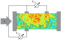
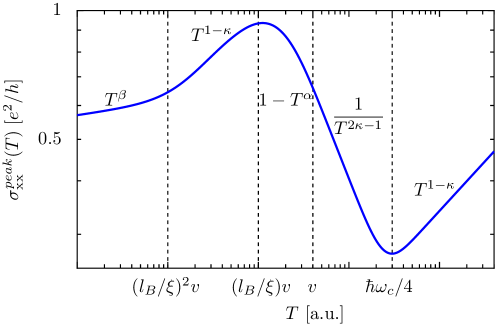
Second, we will present in Sec. 3 a general diagrammatic formalism[14] allowing to compute dissipative transport dominated by classical percolation effects in quantum Hall samples such as depicted in Fig. 1. In particular, we will be able to give strong support to a previously conjectured[11, 12, 13, 15] critical exponent $\kappa=10/13$ for the peak longitudinal conductivity $\sigma_{xx}^{\mathrm{peak}}$ in the high temperature regime of the plateau transition. An universal scaling function describing the crossover for temperatures near the cyclotron energy (see the V-shaped part of the curve in Fig. 1) will be computed, giving a way to extract $\kappa$ from experiments.

2 Classically percolating transport at the plateau transition

2.1 Local conductivity model

The starting point of transport calculations in the high temperature regime of the quantum Hall effect is a purely classical model[11, 14], where the continuity equation $\bm{\nabla}\cdot\mathbf{j}=0$ (i.e. the continuum version of Kirchoff’s law) is solved from the microscopic knowledge of Ohm’s law $\mathbf{j}(\mathbf{r})=\hat{\sigma}(\mathbf{r})\mathbf{E}(\mathbf{r})$, defining here the local conductivity tensor[16, 17] that relates the local electric field to the local current density. Due to the existence of several energy scales, the disorder-induced spatial variations of $\hat{\sigma}(\mathbf{r})$ have a strong temperature dependence, which in turn affects the macroscopic transport properties. Drastic simplifications occur in the regime of high magnetic fields[17, 18], where the combination of Lorentz force and local electrostatic potentials induces a slow drift motion in the direction orthogonal to the crossed magnetic and local electric fields. This vindicates the first simplification of the conductivity tensor

$$\hat{\sigma}(\mathbf{r})=\begin{pmatrix}\sigma_{0}&-\sigma_{H}(\mathbf{r})\\ \sigma_{H}(\mathbf{r})&\sigma_{0}\end{pmatrix},$$ (1)

where $\sigma_{0}$ encodes dissipative processes such as electron-phonon scattering, which will be assumed to be uniform in the bulk of the sample, and $\sigma_{H}(\mathbf{r})$ is the local Hall component, whose spatial dependence originates from charge density fluctuations due to disorder in the sample. We will discuss below the various regimes that can be expected for $\sigma_{H}(\mathbf{r})$ depending on the range of temperature $T$. For this purpose, we need to introduce the energy scales associated with the local disorder potential $V({\bf r})$, and we define its typical amplitude $v=\sqrt{\big{<}[V({\bf r})]^{2}\big{>}}$ and correlation length $\xi$. We will assume throughout that the disorder is smooth at the scale of the magnetic length $l_{B}=\sqrt{\hbar/eB}$ ($l_{B}=8$nm at $B=10$T), so that $l_{B}/\xi$ is a small parameter. In what follows, a centered Gaussian distribution will be considered for the local electrostatic potential $V(\mathbf{r})$. The local conductivity model introduced here is valid at temperatures high enough so that phase-breaking processes, such as electron-phonon scattering, occur on length scales that are shorter than the typical variations of disorder. However, quantum mechanics may still be important to determine the microscopics of the conductivity tensor, as we argue below.

2.2 Percolation effects in quantum Hall transport: phenomenology

The occurence of percolation effects in the quantum Hall regime can be understood already from a quasiclassical perspective. In the high magnetic field limit, cyclotron and guiding center motions fully decouple, giving rise to Landau quantization on one hand, and to mainly closed trajectories of the guiding center on the other hand, that follow the equipotentials of the disorder landscape. Intuitively, the electrical current contributing to macroscopic transport will thus follow a percolation backbone. The crucial role of inelastic processes, controlled by the longitudinal component $\sigma_{0}$ in Eq. (1), can be understood by the fact that such current-carrying extended states must pass through many saddle-points on the disorder landscape. However, the drift velocity associated to the guiding center identically vanishes at these points, so that having a finite $\sigma_{0}$ is essential to connect the different valleys of the potential profile. The technical difficulty lies in evaluating the macroscopic conductivity in the limit where $\sigma_{0}$ is much smaller than the amplitude variations of the Hall component $\sigma_{H}(\mathbf{r})$, but yet does not fully vanish. This regime cannot simply be accessed from the $\sigma_{0}\to 0$ limit, because the transport equation becomes singular. The strategy developped in Ref. FFC2011 and Sec. 3 will be to extrapolate from high orders of the perturbatively controlled $\sigma_{0}\to\infty$ expansion to the case of small dissipation.

Assuming that a critical state is established in the small $\sigma_{0}$ limit due to the scale invariant nature of the percolation backbone, one can infer from dimensional analysis that the macroscopic longitudinal conductivity scales as[11, 14]:

$$\sigma_{xx}\propto\sigma_{0}^{1-\kappa}[\big{<}\sigma_{H}^{2}\big{>}-\big{<}\sigma_{H}\big{>}^{2}]^{\kappa/2},$$ (2)

where $\kappa$ is a non-trivial exponent previously conjectured[11, 12, 13, 15] to be $\kappa=10/13$, see Sec. 3 for a diagrammatic approach to this result. Based on simple microscopic arguments for the local Hall conductivity $\sigma_{H}(\mathbf{r})$ that we introduce now, it is possible to understand from Eq. (2) various transport regimes that are relevant for quantum Hall systems. In all what follows, we will assume that electron-phonon processes dominate in the longitudinal component[19], leading to the temperature dependence $\sigma_{0}(T)\propto T$.

2.3 A hierarchy of transport crossovers

2.3.1 Fully classical regime: $\hbar\omega_{c}\ll T$

At temperatures higher than the cyclotron energy, both cyclotron and drift motions are classical, so that the classical Hall’s law prevails: $\sigma_{H}(\mathbf{r})=(e/B)n(\mathbf{r})$, with $n(\mathbf{r})$ the local electronic density, which undergoes smooth spatial fluctuations in case of high mobility samples[11]. In relatively clean samples, the amplitude $v$ of disorder fluctuations remain small compared to the classical cyclotron energy, so that the Hall conductivity follows at first order the spatial variations of the local potential:

$$\sigma_{H}(\mathbf{r})=\frac{en}{B}+AV(\mathbf{r}).$$ (3)

with $n$ the total electron density and $A$ a constant to be determined below. Thus, for a Gaussian distributed disorder, the local Hall conductivity displays Gaussian fluctuations and is weakly dependent of temperature. Using the percolation Ansatz (2) for the macroscopic longitudinal conductivity, we find:

$$\sigma_{xx}\propto v^{\kappa}T^{1-\kappa}\propto T^{3/13},$$ (4)

which shows already a first non-trivial behavior in temperature[12, 14] connected to classical percolation, where the conductivity mildly decreases as temperature is lowered, see also Fig. 1.

2.3.2 Formation of Landau levels: $v\ll T\ll\hbar\omega_{c}$

As temperature crosses the cyclotron energy, Landau levels start to emerge, and the local density is given by Pauli’s principle: $\sigma_{H}(\mathbf{r})={\displaystyle\frac{e^{2}}{h}}{\displaystyle\sum_{m=0}^{\infty}}n_{F}[E_{m}-V(\mathbf{r})-\mu]$ with $\mu$ the chemical potential and $n_{F}(E)=1/(e^{E/T}+1)$ the Fermi-Dirac distribution (we set Boltzmann’s constant $k_{B}=1$ in what follows). We will neglect spin effects for simplicity in what follows (Landau levels are assumed spin non-degenerate). In the considered temperature range $v\ll T$, the Fermi distribution can be linearized, which leads to Eq. (3) with $A=(e^{2}/h)(\hbar\omega_{c})^{-1}$ in the case $\hbar\omega_{c}\ll T$ considered previously, and more generally to:

$$\sigma_{H}(\mathbf{r})=\frac{en}{B}+\frac{e^{2}}{h}\sum_{m=0}^{\infty}n_{F}^{\prime}(E_{m}-\mu)V(\mathbf{r}).$$ (5)

The local conductivity remains Gaussian, but acquires now an extra temperature dependence from the Fermi function, which can be illustrated in the case of the plateau $\nu\to\nu+1$ transition, which leads for $T\ll\hbar\omega_{c}$ to

$$\sigma_{H}^{\mathrm{peak}}(\mathbf{r})=\frac{en}{B}+\frac{e^{2}}{h}\frac{1}{4T}V(\mathbf{r}).$$ (6)

Using the percolation Ansatz (2), we find in the considered temperature range:

$$\sigma_{xx}^{\mathrm{peak}}\propto\left(\frac{v}{T}\right)^{\kappa}T^{1-\kappa}\propto\frac{1}{T^{2\kappa-1}}\propto\frac{1}{T^{7/13}},$$ (7)

so that the peak longitudinal conductivity strongly increases below $T\lesssim\omega_{c}/4$ (this crossover scale, as well as the complete scaling function will be determined in Sec. 3), see also Fig. 1.

2.3.3 Two-fluids regime: $(l_{B}/\xi)v\ll T\ll v$

The peak longitudinal conductivity cannot diverge at vanishing temperature, and the law (7) must be cut-off by additional physical processes. Indeed, by further lowering the temperature, the Fermi distributions becomes sharp at the scale $T\ll v$, and the local Hall conductivity $\sigma_{H}(\mathbf{r})$ now assumes rapid spatial variations between quantized values $\nu e^{2}/h$ and $(\nu+1)e^{2}/h$, with $\nu$ the filling factor. The local conductivity model now reads

$$\sigma_{H}(\mathbf{r})=\frac{e^{2}}{h}\nu+\frac{e^{2}}{h}\Theta[V(\mathbf{r})+\mu-E_{\nu}],$$ (8)

introducing the step function $\Theta$. The transport properties of this two-fluids model were considered extensively in previous works[20]. It was found using duality arguments that the local conductivity Eq. (8) leads in the (unphysical) limit of zero temperature to an exact value for the longitudinal peak conductivity in the $\sigma_{0}\to 0$ limit: $\sigma_{xx}^{\mathrm{peak}}=e^{2}/h$. This result would seem at first sight at odds with the scaling Ansatz (2), which predicts a powerlaw vanishing of $\sigma_{xx}$ at small $\sigma_{0}$. On mathematical grounds, the model Eq. (8) is quite peculiar in the sense that the fluctuations of the Hall conductivity $[\big{<}\sigma_{H}^{2}\big{>}-\big{<}\sigma_{H}\big{>}^{2}]$ are actually diverging at the peak value, invalidating the Ansatz. Yet, the existence of a finite and universal value $\sigma_{xx}^{\mathrm{peak}}=e^{2}/h$ seems still physically surprising from the argumentation given in Sec. 2.2, where we argued that the fully opened current lines at $\sigma_{0}$ have a vanishing drift velocity at the saddle points of disorder. However, for such bimodal distribution of the local Hall conductivity Eq. (8) and in contrast to any continuous conductivity distribution, the drift velocity does not vanish anymore at the saddle points, which allows to establish a macroscopic current even in the absence of dissipation mechanisms. This simple argument allows to understand why the percolation scaling Ansatz (2) does not apply to the two-fluids model of Dykhne and Ruzin[20]. However, we will see below that other processes invalidate the model Eq. (8) in the limit of zero temperature. Mreover, we can also infer how the “exact” value $e^{2}/h$ is approached from above. Indeed, the sharp Fermi function in Eq. (8) is always smeared on the scale $T$, recovering a continuous (but strongly non-Gaussian) distribution, leading likely to power-law deviations from the exact zero-temperature result $e^{2}/h$:

$$\sigma_{xx}^{\mathrm{peak}}=\frac{e^{2}}{h}-BT^{\alpha}$$ (9)

with a new critical exponent $\alpha>0$ that is to our knowledge still unknown, and $B$ some constant. The fact that the peak longitudinal conductivity levels off at low temperatures towards values close (but not strictly equal) to $e^{2}/h$ has been noted from experimental data[20], see also Fig. 1.

2.3.4 Wavefunction corrections: $(l_{B}/\xi)^{2}v\ll T\ll(l_{B}/\xi)v$

The low-temperature two-fluids conductivity model Eq. (8) relies on the high magnetic field limit, and is strictly speaking only correct in the limit $l_{B}\to 0$. However, quantum corrections will occur for finite $l_{B}/\xi$ due to the fact that the electronic wavefunctions are not infinitely sharp transverse to the guiding center motion, but rather spread on the scale of the magnetic length $l_{B}$. For this reason, the local Hall conductivity $\sigma_{xx}(\mathbf{r})$ will not undergo infinitely sharp steps from a quantized value to the next as in Eq. (8), but rather rapid but smooth rises on the scale $l_{B}$, see Refs.CFC2008,CF2009. Because the wavefunctions extend transversely in a Gaussian manner, the resulting form of the Hall conductivity is easily understood (here for the lowest Landau level):

$$\sigma_{H}(\mathbf{r})=\frac{e^{2}}{h}+\frac{e^{2}}{h}\int\frac{d^{2}\mathbf{R}}{\pi l_{B}^{2}}\;\Theta\left[V(\mathbf{R})-\mu-E_{\nu}\right]e^{-(\mathbf{r}-\mathbf{R})^{2}/l_{B}^{2}}.$$ (10)

Clearly, the two-fluid model Eq. (8) is recovered in the limit $l_{B}/\xi\to 0$, but for a more realistic smooth disorder, the correlation length $\xi$ does not exceed a few hundreds of nanometers. In that case, the sharp step in Eq. (8) is smoothened whenever the new energy scale $(l_{B}/\xi)v$ sets in. Interestingly, we recover now a continuous conductivity distribution where the percolation Ansatz (2) should apply. Because the spatial fluctuations of the local Hall conductivity are no more controlled by temperature, we can infer without detailed calculation the following powerlaw for the peak longitudinal conductivity:

$$\sigma_{xx}^{\mathrm{peak}}\propto T^{1-\kappa}\propto T^{3/13}.$$ (11)

Thus the peak conductivity should decrease again by cooling the sample to very low temperatures, as evidenced experimentally[8], see also Fig. 1.

2.3.5 Onset of quantum tunneling: $T\ll(l_{B}/\xi)^{2}v$

By further cooling towards the limit of zero temperature, a new energy scale $(l_{B}/\xi)^{2}v$ emerges, associated to quantum tunneling at the saddle points[18]. For high mobility samples, one can assume that transport remains incoherent between the widely separated saddle points, so that quantum interference effects can be neglected, and the local conductivity model Eq. (1) still applies (if not, non-local effects in the spirit of Ref. Baranger must be accounted for). Here, the precise form of the local conductivity tensor is not yet fully understood, although a quasilocal approach that incorporates quantum tunneling can be developped[18]. For this reason, the precise scaling form of the peak longitudinal conductivity is still unknown in this regime, although a slower decrease than Eq. (11), leading to a kink at $T=(l_{B}/\xi)^{2}v$, can be expected, due to the onset of the quantum processes allowing to transfer electrons above the saddle points:

$$\sigma_{xx}^{\mathrm{peak}}\propto T^{\beta}\;\;\;\;\;0<\beta<3/13.$$ (12)

Such behavior was also observed experimentally in low temperature studies of the peak longitudinal conductivity[8], see also Fig. 1.

3 Diagrammatic approach to classical percolating transport

3.1 Systematic weak coupling expansion and extrapolation to the percolation regime

Our goal in this section is to discuss how classical percolation features in quantum Hall transport can be captured analytically by a diagrammatic approach[14], allowing to recover the percolation Ansatz (2) and accurate estimates of the critical exponent $\kappa$ discussed in Sec. 2.3. Building on earlier works[22, 23] for the case of the local conductivity tensor Eq. (1), one can show by standard techniques that the disorder averaged longitudinal macroscopic conductivity reads

$$\begin{pmatrix}\sigma_{xx}&-\sigma_{xy}\\ \sigma_{xy}&\sigma_{xx}\end{pmatrix}=\begin{pmatrix}\sigma_{0}&-\big{<}\sigma_{H}\big{>}\\ \big{<}\sigma_{H}\big{>}&\sigma_{0}\end{pmatrix}+\big{<}\hat{\chi}(\mathbf{r})\big{>},$$ (13)

where $\hat{\chi}(\mathbf{r})$ obeys the equation of motion:

$$\hat{\chi}(\mathbf{r})=\delta\sigma(\mathbf{r})\hat{\epsilon}+\delta\sigma(\mathbf{r})\int\!\!\!d^{2}r^{\prime}\,\hat{\epsilon}\,\hat{\cal{G}}_{0}(\mathbf{r}-\mathbf{r^{\prime}})\hat{\chi}(\mathbf{r^{\prime}}).$$ (14)

We have introduced above the Hall conductivity fluctuations $\delta\sigma(\mathbf{r})\equiv\sigma_{H}(\mathbf{r})-\big{<}\sigma_{H}\big{>}$, the antisymmetric $2\times 2$ tensor $\hat{\epsilon}$, and the Green’s function:

$$[\hat{\cal{G}}_{0}]_{ij}(\mathbf{r})=\frac{\partial}{\partial r_{i}}\frac{\partial}{\partial r_{j}}\int\!\!\!\frac{d^{2}p}{(2\pi)^{2}}\frac{e^{i\mathbf{p}\cdot\mathbf{r}}}{\sigma_{0}|\mathbf{p}|^{2}+0^{+}}.$$ (15)

In previous analyses of Eq. (14), several methods were proposed, such as a mean-field treatment[23], lowest order perturbation theory[24] in powers of $\big{<}[\delta\sigma]^{2}\big{>}/\sigma_{0}^{2}$, or self-consistent Born approximation[22]. Clearly these approaches are insufficient to capture the critical percolation behavior in the strong coupling limit $\sigma_{0}\to 0$. However, the small dissipation Ansatz (2) ressembles the critical behavior typical of phase transitions, and leads hope that Padé extrapolation techniques of a sufficiently high order perturbative calculation could bridge the gap from weak (i.e. $\big{<}[\delta\sigma]^{2}\big{>}\ll\sigma_{0}^{2}$) to strong coupling (i.e. $\big{<}[\delta\sigma]^{2}\big{>}\gg\sigma_{0}^{2}$). The calculation actually simplifies for the case of Gaussian fluctuations of the local Hall conductivity $\delta\sigma(\mathbf{r})$, which applies to the highest temperature regimes considered in Eq. (3) and Eq. (5). By symmetry considerations, one finds that the Hall component is not affected in the high temperature regime, namely classical Hall’s law $\sigma_{xy}=en/B$ holds. By dimensional analysis, the longitudinal conductivity reads:

$$\sigma_{xx}=\sigma_{0}+\sum_{n=1}^{\infty}a_{n}\frac{\langle\delta\sigma^{2}\rangle^{n}}{\sigma_{0}^{2n-1}}$$ (16)

with dimensionless coefficients $a_{n}$ collecting all diagrams of order $n$ in perturbation theory in $\langle\delta\sigma^{2}\rangle/\sigma_{0}^{2}$. The longitudinal conductivity $\sigma_{xx}$ thus receives non-trivial corrections that will lead to percolation effects in the limit $\sigma_{0}\to 0$.

The methodology to compute the large $\sigma_{0}$ expansion relies in iterating Eq. (14) to the desired order, averaging over disorder owing to the relation (5), and evaluating the resulting multidimensional integral, either analytically or numerically, see Fig. 2.

Figure 2: Diagrammatic expansion in the case of Gaussian fluctuations of the local conductivity. Wiggly lines are associated to disorder averages, and solid lines to the Green’s function Eq. (15)

In order to simplify the calculations, we considered spatial correlations of disorder of the form $\langle\delta\sigma(\mathbf{r})\delta\sigma(\mathbf{r^{\prime}})\rangle=\langle\delta\sigma^{2}\rangle e^{-|\mathbf{r}-\mathbf{r^{\prime}}|^{2}/\xi^{2}}$, with correlation length $\xi$, allowing us to compute the series Eq. (16) up to sixth loop order[14], see Table 3.1.

Coefficients $a_{n}$ of the perturbative series (16) up to sixth loop order. Order Method Coefficient $a_{n}$ 1 Analytical $\frac{1}{2}$ 2 Analytical $\frac{1}{8}-\frac{1}{2}\log(2)$ 3 Analytical $0.2034560502$ 4 Numerical $-0.265\pm 0.001$ 5 Numerical $0.405\pm 0.001$ 6 Numerical $-0.694\pm 0.001$

Standard extrapolation techniques allow us to extract[14] the estimate $\kappa=0.767\pm 0.002$ for the critical exponent appearing in Eq. (2), quite close to the previously conjectured value[11, 12, 13, 15] $\kappa=10/13\simeq 0.769$.

3.2 High temperature crossover function for $\sigma_{xx}^{\mathrm{peak}}$

We finally provide a simple scaling function describing the crossover from the high temperature regime above the cyclotron energy $T\gg\hbar\omega_{c}$ to the intermediate situation $v\ll T\ll\hbar\omega_{c}$, where Gaussian fluctuation of the local Hall conductivity still arise, see Eq. (5). From this expression, we can connect the typical fluctuations of the Hall conductivity to the width $v=\sqrt{\big{<}[V({\bf r})]^{2}\big{>}}$ of the disorder distribution: $\sqrt{\big{<}[\delta\sigma({\bf r})]^{2}\big{>}}={\displaystyle\frac{e^{2}}{h}}v\Bigg{|}{\displaystyle\sum_{m=0}^{\infty}}n_{F}^{\prime}(E_{m}-\mu)\Bigg{|}$, so that the high temperature crossover function reads from the scaling Ansatz (2):

$$\sigma_{xx}=\sigma_{0}^{1-\kappa}\left|\frac{e^{2}}{h}v\sum_{m=0}^{\infty}n_{F}^{\prime}(E_{m}-\mu)\right|^{\kappa}.$$ (17)

Note that for the Gaussian model studied here, a dimensionless prefactor in Eq. (17) happens[14] to be quite close to 1, and has not been written. At temperatures such that $v\ll T\ll\hbar\omega_{c}$ and at the $\nu\to\nu+1$ plateau transition, i.e. for $\mu=\hbar\omega_{c}(\nu+1/2)$, we thus find:

$$\sigma_{xx}^{\mathrm{peak}}=\sigma_{0}^{1-\kappa}\left|\frac{e^{2}}{h}\frac{v}{4T}\right|^{\kappa},$$ (18)

recovering expression (7) for the longitudinal conductivity in the limit $v\ll T\ll\hbar\omega_{c}$.

We can alternatively re-express the sum over Landau levels in Eq. (17) by using Poisson summation formula[25] in the limit $T<\mu$, giving:

$$\sigma_{xx}=\sigma_{0}^{1-\kappa}\left[\frac{e^{2}}{h}\frac{v}{\hbar\omega_{c}}\Bigg{|}1+\sum_{l=1}^{+\infty}(-1)^{l}\cos\left(\frac{2\pi l\mu}{\hbar\omega_{c}}\right)\frac{\frac{4\pi^{2}lk_{B}T}{\hbar\omega_{c}}}{\mathrm{sinh}\left(\frac{2\pi^{2}lk_{B}T}{\hbar\omega_{c}}\right)}\Bigg{|}\right]^{\kappa}$$ (19)

vindicating expression (4) for the peak longitudinal conductivity in the $T\gg\hbar\omega_{c}$ limit. Either Eq. (17) or Eq. (19) can be used to extract the critical exponent $\kappa$ from experimental data in the range of temperatures near the cyclotron energy.

4 Perspectives

As a conclusion, we list several issues that could be addressed in further developments of the present work.

• What is the magnetic field behavior of $\sigma_{xx}$ at high temperature?

• Can one extract reliably the classical exponent $\kappa$ from experiments?

• Are the exponents $\alpha$ and $\beta$ of the low temperature regime related to $\kappa$?

• How do the finite probe currents affect the Hall plateau quantization?

• What are the fundamental differences between 2DEGs and graphene[26]?

• Is a more realistic description of electron-phonon conductivity[19] needed?

• Can one describe the crossover to Drude behavior at low magnetic fields[27]?

• Can one implement transport calculations using diagrammatic QMC [28]?

References

- [1] K. Von Klitzing, G. Dorda, and M. Pepper, Phys. Rev. Lett. 45, 494 (1980).
- [2] R. E. Prange and S. M. Girvin, The Quantum Hall Effect, (Springer, New York, 1987).
- [3] M. Janssen, O. Viehweger, U. Fastenrath, and J. Hadju, Introduction to the Theory of the Integer Quantum Hall Effect (VCH, Germany, 1994).
- [4] J. Matthews and M. E. Cage, J. Res. Natl. Inst. Stand. Technol. 110, 497 (2005).
- [5] B. Huckestein, Rev. Mod. Phys. 67, 357 (1995).
- [6] B. Kramer, T. Ohtsuki and S. Kettemann, Phys. Rep. 417, 211 (2005).
- [7] F. Evers and A. D. Mirlin, Rev. Mod. Phys. 80, 1355 (2008).
- [8] H. P. Wei et al., Phys. Rev. B 45, 3926 (1992).
- [9] W. Li et al., Phys. Rev. B 81, 033305 (2010).
- [10] K. Hashimoto et al., Phys. Rev. Lett. 101, 256802 (2008).
- [11] S. H. Simon and B. I. Halperin, Phys. Rev. Lett. 73, 3278 (1994).
- [12] D. G. Polyakov and B. I. Shklovskii, Phys. Rev. Lett. 74, 150 (1995).
- [13] M. M. Fogler and B. I. Shklovskii, Sol. State Comm. 94, 503 (1995).
- [14] M. Flöser, S. Florens, and T. Champel, Phys. Rev. Lett. 107, 176806 (2011).
- [15] M. B. Isichenko, Rev. Mod. Phys. 64, 961 (1992).
- [16] M. R. Geller and G. Vignale, Phys. Rev. B 50, 11714 (1994).
- [17] T. Champel, S. Florens and L. Canet, Phys. Rev. B 38, 125302 (2008).
- [18] T. Champel and S. Florens, Phys. Rev. B 80, 125322 (2009).
- [19] H. L. Zhao and S. Feng, Phys. Rev. Lett. 70, 4134 (1993).
- [20] A. M. Dykhne and I. M. Ruzin, Phys. Rev. B 50, 2369 (1994).
- [21] H. U. Baranger and A. D. Stone, Phys. Rev. B 40, 8169 (1989).
- [22] Y. A. Dreizin and A. M. Dykhne, Sov. Phys. JETP 36, 127 (1972).
- [23] D. Stroud, Phys. Rev. B 12, 3368 (1975).
- [24] C. Timm, M. E. Raikh and F. von Oppen, Phys. Rev. Lett. 94, 036602 (2005).
- [25] T. Champel and V. P. Mineev, Philos Mag. B 81, 55 (2001).
- [26] T. Champel and S. Florens, Physical Review B 82, 045421 (2010).
- [27] D. G. Polyakov, F. Evers, A. D. Mirlin and P. Wölfle, Phys. Rev. B 64, 205306 (2001).
- [28] E. Gull et al., Rev. Mod. Phys. 83, 349 (2011).