A study of atom localization in an optical lattice by analysis of the scattered light

Abstract

We present an experimental study of a four beam optical lattice using the light scattered by the atoms in the lattice. We use both intensity correlations and observations of the transient behavior of the scattering when the lattice is suddenly switched on. We compare results for 3 different configurations of the optical lattice. We create situations in which the Lamb-Dicke effect is negligible and show that, in contrast to what has been stated in some of the literature, the damping rate of the ’coherent’ atomic oscillations can be much smaller than the inelastic photon scattering rate.

I Introduction

In the past five years, optical lattices have attracted a great deal of experimental and theoretical interest jessen2 . Beginning with studies of the quantized motion of atoms in the sub-micron sized potential wells verkerk1 ; jessen1 , many workers have succeeded in observing a large variety of effects and are now beginning to investigate the transport properties, both classical and quantum in these systems courtois2 ; jurczak2 ; anderson ; marksteiner2 .

There are several methods of observation of optical lattices, and among them two groups, including ours, recently demonstrated that intensity correlation, a well established technique in other fieldsChu , can be used to gain informationjurczak1 ; bali . Although the bulk of our new results has been related to the transport properties of atoms in these lattices (i.e. the motion from well to well) jurczak2 , our experiment, like many others, also gives information about the motion of atoms inside the wells. In this paper we will detail our results on this motion and use our data to confirm recent ideas grynberg ; comment about the damping mechanisms which affect the motion of atoms inside the lattice potential wells.

A novel feature in our experiment is that we can study the behavior of atoms in a tetrahedral optical lattice for a large range of beam angles. This feature has already permitted us to study transport by density waves in lattices as a function of lattice anglejurczak3 . Here we will discuss a study of the intrawell dynamics, i.e. the oscillation of atoms inside a single well as a function of lattice angle.

In addition to the intensity correlation measurements, we have also studied the same dynamics by observing the atomic fluorescence as a function of time after a homogeneous atomic sample is suddenly subjected to an optical lattice. Although not as powerful a method as Bragg scattering for studying the localization of atoms in individual wells, we demonstrate in the appendix that a fairly simple experiment is indeed sensitive to the degree of localization in a single well.

II Theoretical Remarks

In our experiments we used a 4-beam optical lattice configuration introduced in Ref. verkerk2 . The configuration of laser beams and polarizations is shown in Fig. 1. We denote by $\theta$ the half angle between the lattice beams in the $x-z$ and $y-z$ planes. The $x-z$ and $y-z$ angles were always the same. The resulting electric field and optical potential are discussed in detail in Ref. petsas . Here we will simply state the results of this work which are important for our study. For an atom with an F_g=3 ground state and an F_e=4 excited state, Montecarlo wavefunction simulationsmarksteiner raithel have shown that atoms in the lattice are rapidly pumped into the extreme magnetic sublevels $m_{F}=\pm 3.$ Therefore we will neglect the potentials not corresponding to these two states. The three dimensional light shift potential for atoms in the m_F =$\pm$3 state is given by:

$$U_{\pm}=-\frac{U_{0}}{4}\left(\frac{29}{28}\left(\cos^{2}(k_{x}x)+\cos^{2}(k_{y}y)\right)\mp\frac{27}{28}\left(2\cos(k_{x}x)\cos(k_{y}y)\cos(2k_{z}z)\right)\right)$$ (1)

Where $k_{x}=k_{y}=k\sin\theta,$ $k_{z}=k\cos\theta$ , $k=2\pi/\lambda$ is the wavevector of the light and $U_{0}$ is the light shift at the bottom of the potential well. The numerical factors come from the values of the Clebsch Gordan coefficients. In the large detuning limit this light shift is related to the saturation parameter $s_{0}=\frac{\Omega_{R}^{2}}{2}/\left(\Delta^{2}+\frac{\Gamma^{2}}{4}\right)$ of a single laser beam by $U_{0}=4\hbar\Delta s_{0},$ with $\Omega_{R}$ being the Rabi frequency, $\Delta$ the detuning and $\Gamma$ the natural linewidth. From the curvature of the bottom of these wells one can calculate an oscillation frequency along each axis for an atom near the bottom of each well:

$$\Omega_{x,y} = \omega_{R}\sqrt{\frac{2U_{0}}{E_{R}}}\sin\theta$$ (2)

$$\Omega_{z} = 2\omega_{R}\sqrt{\frac{28}{27}\frac{U_{0}}{E_{R}}}\cos\theta$$ (3)

Here $E_{R}=\frac{\hbar^{2}k^{2}}{2m}$ denotes the recoil energy, and $\omega_{R}=E_{R}/\hbar.$

Figure 1: Configuration of laser beams and polarizations used to create the optical lattice used in this experiment. The heavy arrows show the beam propagation directions and the fine arrows the polarizations.

These oscillation frequencies have been observed using many different methods. Our intensity correlation technique amounts to observing the beat note between the light radiated by different atoms. Since the atoms are oscillating at well defined frequencies, the power spectrum of the emitted electric field contains a ’carrier’ at the laser frequency and sidebands separated by multiples of the oscillation frequency. Thus the ’self-beating’, or intensity correlation spectrum contains beat notes at these frequencies. Instead of self-beating one can also use a local oscillator (heterodyning) to observe the sidebands jessen1 ; gatzke ; westbrook . Both of these methods can also be considered as spontaneous Raman spectroscopy of the vibrational levels in the potential wells. In pump-probe spectroscopy, on the other hand, verkerk1 ; hemmerich2 one observes stimulated Raman transition between the energy levels in the wells. Four-wave mixing signals also contain motional sidebands hemmerich . Recently various groups have observed oscillations in a transient way, by non-adiabatically changing the potential wells and observing the motion either through the redistribution of photons in the lattice beams kozuma ; phillipspc or using Bragg scattering raithel ; raithel2 ; gorlitz .

In the first discussions of the motion of atoms inside the potential wells of an optical lattice, attention was drawn to the fact that the motional sidebands, which were the signature of a well defined oscillation of the atoms in the wells, appeared to be narrower than the simplest expectation verkerk1 ; jessen1 . Naively, one expects the linewidth of such a system to be approximately equal to the total photon scattering rate (at the bottom of a well this rate is given approximately by $\frac{U_{0}}{\hbar\Gamma}\Delta$). References verkerk1 ; jessen1 , however, pointed out that in fact only the inelastic scattering rate (the rate of scattering events involving a change of the quantum state of the atom) should determine that linewidth. Because the experiments were in the Lamb-Dicke regime, i.e. the amplitude of the oscillation was much smaller than the wavelength of the emitted radiation, inelastic scattering was strongly suppressed in these experiments wineland ; courtois , and this accounted for the observed width.

This argument is roughly correct if there is no significant excitation of the harmonic oscillator, i.e. most of the atoms are in the ground state, as was indeed approximately true in the experiments of Refs. verkerk1 ; jessen1 . Later, however, Ref. grynberg pointed out that when the amplitude of the atomic oscillation is large enough that one must include the effects of many levels in the well, there is a transfer of coherence mechanism which suppresses the linewidth even further. Essentially, this mechanism involves the fact that although coherences between adjacent levels in a well do decay at a rate determined by the inelastic scattering rate, these coherences are also ’fed’ by other, higher lying coherences, provided that the higher lying coherences oscillate at approximately the same frequency as the lower lying ones, i.e. that the well is nearly harmonic.

Indeed, in the case of a perfectly harmonic well, Ref. cct demonstrates that the coherence transfer mechanism works in such a way that the linewidth of the oscillator is determined only by the rate at which energy is extracted from the oscillator through its coupling to a thermal reservoir, and not by the decay rates of the individual coherences. This extraction rate is exactly the same as the damping, or cooling rate of the classical oscillator.

The case of the perfectly harmonic oscillator was adapted to the case of laser cooling in Ref. comment to explain the damping rates observed in an experiment reported in Ref. kozuma . The authors of Ref. kozuma used two beams crossing each other at a small angle to produce a one dimensional optical lattice with a very large period (about 5 times the optical wavelength). Thus there was no Lamb-Dicke effect. The experiment, however, showed clear oscillations which damped out much more slowly than the inelastic scattering rate. Because the laser beam polarizations were parallel to each other the atoms behaved nearly like two level systems in the lattice and a Doppler cooling model was enough to show that this result was not surprising. In the case of Doppler cooling one can show that the mean occupation number of the harmonic oscillator $\left\langle n\right\rangle$ is equal to the inelastic scattering rate divided by the energy damping rate due to Doppler cooling. Thus $\langle n\rangle\gg 1$ implies a damping rate much smaller than the inelastic scattering rate, and sidebands narrow compared to the inelastic scattering rate. This result was also stated in Ref. cirac .

For lattices in which the internal structure of the atom plays a significant role in the cooling process (e.g. Sisyphus cooling), the Doppler model is clearly not adequate. But as long as the motion of the atoms at the bottom of the wells in an optical lattice is well described by a damped harmonic oscillator, this damping rate determines the fundamental limit to the width of the sidebands. (Note that Ref. raithel observed a damping rate which may be this fundamental rate. It is not yet clear, however, that the motion can be described simply as a harmonic oscillator.) In what follows we will show experiments in an optical lattice with Sisyphus cooling which confirms these ideas. We show that the inelastic scattering rate, i.e. the Lamb-Dicke parameter, has little to do with the width of the sidebands observed.

III Intensity Correlation Spectroscopy

As we have already mentioned, in correlation spectroscopy, one observes the beating between the light emitted by different atoms in the source. Here we will briefly review some of the ideas underlying intensity correlation spectroscopy; the reader is referred to Refs. jurczak1 ; jurczakth ; westbrook2 ; cummins for more detailed information. We use a spectrum analyser to record the power spectrum $P_{i}(\omega)$ of a detected photocurrent $i(t)$. The Wiener-Khinchine theorem states that $P_{i}(\omega)$ is proportional to the Fourier transform of the correlation function of the photocurrent $\langle i(t)i(t+\tau)\rangle$. If we consider the light as a classical field, the photocurrent is proportional to the incident light intensity $I$ and our observation amounts to a measurement of the normalized correlation function $g_{2}\left(\tau\right)$ of the scattered light intensity:

$$g_{2}(\tau)=\frac{\langle I(t)I(t+\tau)\rangle}{\langle I(t)^{2}\rangle}$$

where $\langle\rangle$ denotes a statistical average. Examples of the spectral and time domain data are shown in Fig. 2. The spectrum (a) and the correlation function (b) were taken using the same optical lattice, in one case using a spectrum analyser and in the other using a digital correlator. In 2(a) we have normalized the spectrum to that of a shot-noise limited light source of the same average intensity, using a procedure described in Ref. jurczak1 . Thus a power density greater than 1.0 represents an ’excess noise power’ which is due to the atoms. In 2(b) we plot $g_{2}\left(\tau\right)-1$. For large values of $\tau$, this function tends to zero.

Figure 2: (a) Intensity correlation spectrum of atoms in an optical lattice, showing a peak at zero frequency corresponding to elastic scattering and a second peak (marked $\Omega_{x}$) at 100 kHz due to spontaneous Raman scattering by atoms changing their level in the potential well. The angle of the lattice was $\theta=30^{\circ}$, the observation direction was along $x$, the detetected light polarization was along $y$, and the detuning was $\Delta=-5\Gamma.$ (b) The autocorrelation function of the light as recorded by a digital correlator under similar conditions.

If one is observing a large number of independent scatterers one can show that the intensity correlation function is related to the correlation function of the electric field $E$ by

$$g_{2}(\tau) = 1+\left|g_{1}(\tau)\right|^{2}$$ (4)

$$g_{1}(\tau) = \frac{\left\langle E^{-}(t)E^{+}(t+\tau)\right\rangle}{\left\langle E^{-}(t)E^{+}(t)\right\rangle}$$

where $E^{\pm}$ refers to the positive and negative frequency components of the electric field. The Fourier transform of $g_{1}(\tau)$ is proportional to the optical power spectrum, and this is the quantity that is measured in heterodyne experiments. From Eq. 4 it is easy to see why the power spectrum of the photocurrent is proportional to the autoconvolution of the optical power spectrum. The fact that we are dealing with an auto-convolution, however, presents some difficulties in the quantitative interpretation of the spectra. For example, the zero frequency peak in our spectrum consists of the autoconvolution of the carrier plus the autoconvolution of the sidebands. Thus its lineshape is complex. In what follows we shall use a Montecarlo simulation to extract quantitative information from our spectra.

IV Description of the experiment

We begin by collecting atoms in a vapor cell Magneto-Optical Trap (MOT) with a Rb partial pressure of order 10^-8hPa. The lasers are tuned slightly to the red of the F_g=3$\rightarrow$F_e=4 component of the D₂ resonance line of ⁸⁵Rb ($\lambda=780$ nm, $\Gamma/2\pi=5.9$ MHz). We can load of order 3$\times 10^{7}$ atoms into the trap with a time constant of a few seconds. After loading the MOT, we switch off both the magnetic field and the trapping beams and turn on the 4 lattice beams. These beams come from a separate diode laser which is injected by the same master laser as the trap laser. The density of atoms in the lattice is approximately 2$\times 10^{9}$ cm^-3. We allow the atoms to equilibrate in the lattice for 5 ms before beginning the data acquisition period. All the lattice beams enter the vacuum chamber by one of two large windows on the sides. Our geometry permits angles $\theta$ as large as 40^∘. This angle could be changed fairly easily and in our experiments we compared values of 20^∘, 30^∘ and 40^∘. These angles were measured with a precision of approximately 1^∘.

We measured the temperature of the atoms in our lattice by releasing the atoms and monitoring their time of flight to a probe beam placed 18 mm below the lattice (the $y$-axis is vertical). For a lattice angles of 30^∘ we recorded the mean energy as a function of the depth of the potential. We determined the potential depth by measuring the oscillation frequency of the atoms and using Eq. 2 and including a 10% anharmonicity correction (see below). The results are shown in Fig. 3. As expected, the temperature depends linearly on the light shift. A linear fit to the data gives:

$$\frac{k_{B}T}{2}=0.17U_{0}+60E_{R}$$ (5)

This result corresponds closely to the results of Ref. gatzke ; kastberg , which studied a 3D lattice at $\theta=45{{}^{\circ}}$ for Cs; both the slope and the intercept seem to be somewhat higher in our case. This discrepancy my be due to differences in the angle of the lattice. Although Ref. kastberg reported that the temperatures were isotropic to within 20%, our 2D simulations of the motion of atoms with a $J_{g}=1/2\rightarrow J_{e}=3/2$ structure jurczakth ; jurczak4 show, for lattice angles of 20^∘ or 30^∘, that the temperature is anisotropic with the $x$ direction a factor of 1.5 hotter than the $z$ direction. The fact that our measurements of the temperature along $x$ are above those reported in Ref. gatzke ; kastberg seems to bear this out bfield .

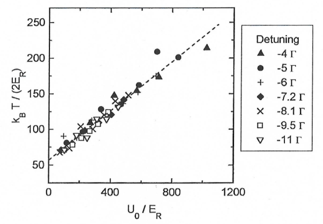
Figure 3: Temperature of atoms in a lattice with $\theta=30^{\circ}$ measured by time of flight as a function of the depth of the potential wells.

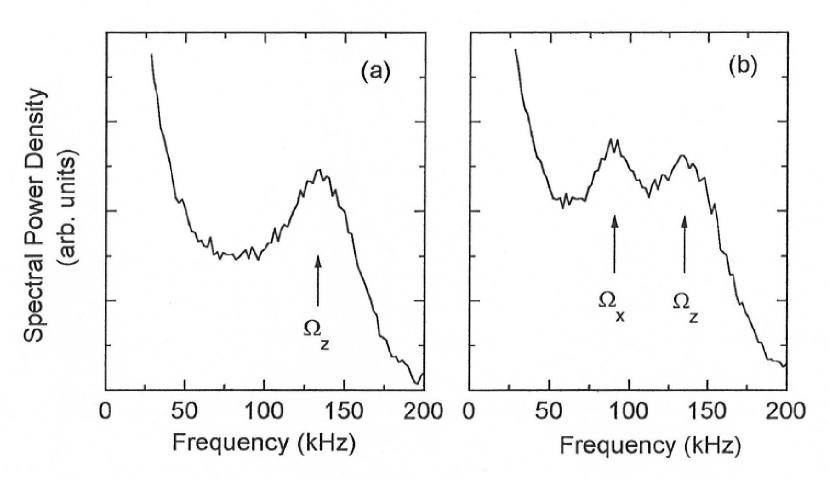
Figure 4: Intensity correlation spectrum of a lattice with $\theta=40^{\circ}.$ (a) Observation along the $z$-axis, (b) Observation direction in the $x-z$ plane at 10 degrees with respect to the $z$-axis. The detected polarization was linear along $y$, and $\Delta=-5\Gamma$

In the correlation experiments, the light scattered by the atoms was detected by avalanche photodiodes with integrated amplifiers and discriminators. These signals were sent either to an FFT spectrum analyser, or a digital correlator. The detection solid angle was approximately 10^-6 sr. Typical count rates were of order 10⁵ to 10⁶ s^-1. The detectors were capable of a maximum count rate of 10⁶ s^-1 without significant saturation. The detector dark count rate was approximately 250 s^-1 and the background count rate, mostly due to scattering of the laser beams by the vapor was of order 10⁴ s^-1. When acquiring correlation data, we typically loaded the MOT for 200 ms and used a data acquisition period of 100 ms during which atom losses were negligible. The measurement cycle was repeated and averaged 10² to 10⁵ times.

V Results

V.1 Measurement of the oscillation frequencies

Figure 4 shows two intensity correlation spectra taken from an optical lattice with $\theta=40{{}^{\circ}}$. In (a) the detection direction was the $z$ axis of Fig.1. In (b) we used a detection angle of 10^∘ from the $z$ direction. We see that when one observes the light scattered along one of the axes of symmetry of the lattice one sees only an oscillation in the direction of that axis (see, however, Ref. jurczak3 for an exception). When another observation direction is chosen one sees both of the eigenfrequencies of the lattice. Note that the positions of the resonances do not change when the observation angle is varied.

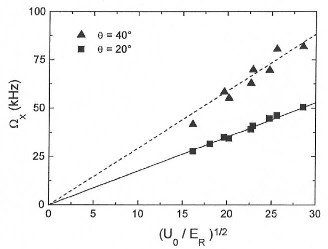
Figure 5: Measurements of the observed oscillation frequency as a function of the square root of the potential well depth. We show the results for two lattice angles. The dependence is linear as expected. The straight lines are fits to the data (see text).

When the lattice angle is changed the two eigenfrequencies change according to Eq. 2, smaller lattice angles leading to more widely spaced frequencies. Fig. 5 shows our measurements of the dependence of oscillation frequency predicted by Eq.2. When we fit the data to a straight line $\Omega_{x}=C\omega_{R}\sqrt{2E_{R}/U_{0}}\sin\theta$, we find $C=0.8$ and $C=0.9$ for $\theta=40^{\circ}$ and $\theta=20^{\circ}$ respectively. Our precision is limited by our 10% uncertainty in the laser intensity. Thus our measurements are marginally consistent with Eq. 2 in which $C=1$. However, we expect that the anharmonicity of the potential should reduce the expected value of $C$ by of order 20%gatzke .

We have also made a systematic study of the relative positions of the two resonances when they are measured simultaneously by observing the spectrum at a small angle relative to $z$. The ratio should be much less sensitive to uncertainties in the absolute measurement of $U_{0}$. A comparison between our measurements and Eq.2 is shown in Table 1 for the angles we tested. As has already been demonstrated in verkerk2 , we find good agreement between the predicted and measured ratios. A theoretical investigation of the role of the potential anharmonicity, as well as the possibly anisotropic temperature would be very useful to refine the comparison with our results.

Table 1: Measured and predicted ratios of the oscillation frequencies along $x$ and $z$ for different lattice angles.

	$\Omega_{x}/\Omega_{z}$
Angle (degrees)	Predicted	Measured
20	0.25	0.26
30	0.40	0.41
40	0.58	0.60

V.2 Width of the vibrational lines

Our ability to vary the angles of the lattice beams allows us not only to vary the oscillation frequency, but also the degree of localization of the atoms in the wells. By localization we mean the rms size of the atomic distribution in a well. Note that several studies have shown marksteiner ; gatzke ; jurczakth that for constant geometry, the rms size of the atomic distribution is unchanged as the depth of the potential is varied. This is because over a large range of parameters the temperature of the atoms is proportional to the well depth. However, the rms size varies with the size of the potential well, assuming that the mean energy of the atoms remains roughly the same. Thus we can observe the behavior of the width of the lines as the rms size is varied.

For the values of the lattice angle available to us, the largest variation in the size of the potential is along $x$ or $y$. In Fig. 6 we show the intensity correlation spectra along the $x$-direction for the angles $\theta$ of 20^∘, 30^∘ and 40^∘ along with a contour plot of the optical potential in the $x-z$ plane (for $y=0$). The contour plots clearly show how the size of the potential varies as a function of angle. The spectra were all taken for the same values of intensity and detuning (i.e. of $U_{0}$ and the light scattering rate). The qualitative features of these spectra can be resumed as follows: As the angle $\theta$ decreases, the oscillation frequencies become smaller, the intensities of the sidebands relative to the peak at zero frequency become larger, the width of the peaks gets slightly smaller, and more vibrational lines become visible.

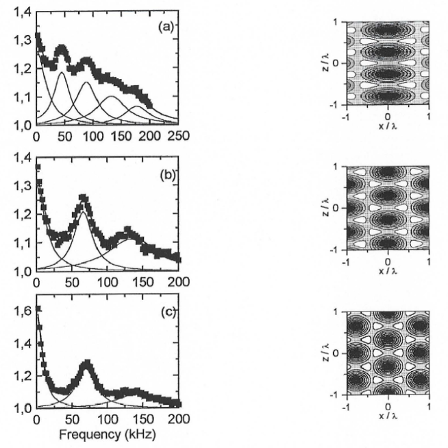
Figure 6: Intensity correlation spectra observed for lattice angles of (a) 20^∘, (b) 30^∘ and (c) 40^∘. For each spectrum $\Delta=-5\Gamma,$ the observation direction was along $x$, and the detected light polarization was along $y$. Next to each spectrum is shown a contour map of the light shift potential, showing the anisotropy of the potentials.

The qualitative interpretation of most these effects is also straightforward. The vibrational frequencies are of course larger in the smaller, stiffer potential wells. Secondly, as the stiffness of the well is reduced, and if the average energy of the atoms remains constant, one also expects that the rms size of the atom distribution increases thus reducing the Lamb-Dicke effect. Therefore one expects the ratio of the intensities radiated into the sidebands and to that in the elastic peak to increase. A reduced Lamb-Dicke effect also favors the appearance of higher harmonics in the vibrational spectra, although we note that if a third harmonic is present in the data for 40^∘ it would not appear in the observed frequency range.

The last feature of the sidebands, their width, is difficult to understand if one holds the view that the width of the sidebands is due to inelastic scattering of the lattice light by the atoms. The fact that the ratio of the height of the sidebands to that of the zero frequency peak increases as the angle is decreased, shows that indeed the Lamb-Dicke effect is being reduced, yet the width of the sidebands is going down. Note that Refs. jurczak2 ; gatzke have already pointed out that the widths of the sidebands in optical lattices seem to be smaller that what would be predicted by the inelastic scattering rate.

To be more quantitative, we would like a measurement of the value of $x_{rms}$ the rms size of the distribution along the $x$ axis for the different situations of Fig 6. One way to do this is to use the ratio ${\cal R}_{C}$ of the total power observed in the sidebands to that of the elastic peak in the intensity correlation spectrum, to find the value of the Lamb-Dicke parameter. Note that this ratio is not the same as the ratio ${\cal R}_{H}$ of the optical power in the sidebands to that in the elastic peak as measured by the heterodyne method gatzke . In the limit of strong localization ($kx_{rms}\ll 1$) one can easily show that jurczakth :

$$(kx_{rms})^{2}=\frac{{\cal R}_{C}}{2}={\cal R}_{H}.$$

In our situation, however, $kx_{rms}$ is not small and therefore to relate $kx_{rms}$ to ${\cal R}_{C}$ we have simulated our experiment using our 2D Montecarlo simulation of a $J_{g}=1/2\rightarrow J_{e}=3/2$ atom. We find that even for angles of 30^∘ and 40^∘ the relation above is approximately valid, and for $\theta=20^{\circ}$ $\frac{{\cal R}_{C}}{2}$ gives an underestimate of $kx_{rms}$. The results of our simulations are summarized in Table 2. In both the simulation and the measurement we estimate ${\cal R}_{C}$ from the spectrum by fitting the data to the sum of several Lorentzians, one for each vibrational sideband as shown in Fig. 6. Although this is not strictly the correct fitting function, (see jurczakth ), the fits are quite good and we believe that the relative areas give a good account of the relative areas of the elastic and inelastic peaks.

Another way to estimate $kx_{rms}$ is to take the measured value of the temperature, Eq. 3, and use the formula for the potential energy, Eq. 2. Then we use

$$\frac{k_{B}T}{2}=\frac{1}{2}m(\Omega_{x}x_{rms})^{2}=\frac{1}{2}U_{0}(k\sin\theta\;x_{rms})^{2}$$ (6)

where $m$ is the mass of the atom. For $\theta=30^{\circ}$ we can make this comparison and as shown in the last column of Table 2 this estimate of $kx_{rms}$ is in reasonable agreement with the one from the spectrum.

Table 2: A comparison of different methods of determing the Lamb-Dicke parameter. The first two columns come from a numerical sumulation. They show that for 30^∘ and 40^∘ the quantity ${\cal R}_{C}$, the ratio of the inelastic to elastic peak intensities in the correlation spectrum, can be used to determine the value of $(kx_{rms})^{2}$. The third column shows the data deduced from Fig. 6, and the fourth column shows the value of $(kx_{rms})^{2}$ determined by the temperature measurements shown in Fig. 3 and using Eq. 6. The internal consitency of these results shows that for $\theta=30^{\circ}$ and $40^{\circ}$ the Lamb-Dicke parameter increases as expected and that for $\theta=20^{\circ}$ our determination of $(kx_{rms})^{2}$ using ${\cal R}_{C}$ is likely to be an underestimate.

	Simulation		Measurement
Angle (degrees)	$\mathcal{R}_{\mathrm{C}}/2$	$(kx_{\mathrm{rms}})^{2}$	$\mathcal{R}_{\mathrm{C}}/2$	$(kx_{\mathrm{rms}})^{2}$
20	3.8	6.5	2.2	—
30	2.5	2.5	1.8	2.2
40	1.9	1.7	1.3	—

Thus we see that in all our experiments the Lamb-Dicke parameter is greater than unity and thus one does not expect Lamb-Dicke narrowing to be present at all. Nevertheless our light scattering rate is approximately $1.5\times 10^{6}$ s^-1 while the width of the sidebands is about $2\times 10^{5}$ s${}^{-1}.$ In addition, while we increased the Lamb-Dicke parameter by about a factor of 3, the width of the sidebands became slightly narrower. The fact that the sideband width is so small even in the absence of Lamb-Dicke narrowing supports the idea that the intrinsic or ’radiative’ width of these lines is governed by the damping rate of the atoms in the harmonic potential and is quite small. We reiterate that the observed width is probably due to the anharmonicity of the potential. Our Montecarlo simulations, in which the atoms’ motion is treated classically show comparable widths.

V.3 Effects of polarization

So far, we have not discussed the polarization of the detected light. Note that in our laser beam configuration, the electric field creating the lattice is $\sigma$ polarized (orthogonal to the $z$-axis) everywhere. When we observe the spectrum along $z,$ the scattered light polarization is of course also $\sigma$, and we observe qualitatively the same spectrum regardless of whether the detection polarization is $\sigma^{+}$, $\sigma^{-},$ $x$ or $y$ (see jurczakth for more details). When observing the light scattered along the $x$-axis, however, one can choose to observe either $\sigma$ or $\pi$ polarized light. In Figs. 2 and 6 we have shown data taken with $\sigma$ polarization.

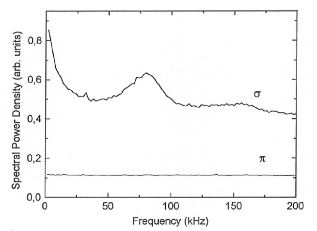
Figure 7: Spectral power density measured along the $x$-direction for two polarization directions. The curve marked $\sigma$ corresponds to a detection polarization along $y$. (as in Figures 2 and 6). The curve marked $\pi$ corresponds to detection of light polarized along the $z$ axis. For both spectra $\theta=30^{\circ}$ and $\Delta=-5\Gamma.$

Surprisingly, the $\pi$ polarized spectrum shows no structure. There is not even a zero frequency peak. We believe this is because by selecting $\pi$ polarized light, we have completely eliminated all elastic scattering: absorption of a $\sigma$ polarized photon followed by the emission of a $\pi$ polarized one necessarily involves a change of the internal state of the atom. Thus one expects this process to have an intrinsic width governed by the inelastic light scattering rate polder . There is also an additional broadening mechanism, due to the fact that selecting the emitted light polarization probably also corresponds to detecting light scattered by atoms which are far from the minima of the potential wells. (In order to emit a $\pi$ polarized photon, an atom in the $m_{F}=+3$ state must absorb a $\sigma^{-}$ photon, and the $\sigma^{-}$ intensity increases as one moves away from the bottom of the $\sigma^{+}$ well.) Thus we are selecting hot atoms, many of which have an energy too large to be trapped by the potential wells. This radiation will thus be Doppler broadended by the motion of these atoms.

VI Conclusions

We have shown that intensity correlation measurements can give a great deal of information about the motion of atoms in optical lattices. Our most important results concern how the characteristics of the correlation spectrum behave when the angles of the lattice are varied. The oscillation frequencies obey a simple law which can be derived from the curvature of the potential wells. Because the lattice angle governs the size of the potential wells we also vary the Lamb Dicke parameter of the atoms in the lattice. We clearly show that varying the Lamb-Dicke parameter has little impact on the width of the motional sidebands. We hope our data will be useful for testing future theoretical treatments, for example taking into account the 3D nature of the problem. The question of what determines the structure of the spectrum of the $\pi$ polarized light remains an interesting problem. To get more experimental information it will be necessary to acquire data over a much larger spectral bandwidth. Correlation measurements in the time domain are well adapted to this type of measurement.

We thank J.-Y. Courtois for valuable discussions. W.D.P thanks NATO and the CNRS for support and hospitality. G.B. was supported by E.U.grant ERB CHBG-CT93-0436. This work was supported by DRET and by E.U.grant ERB FMRX-CT96-0002.

¹present address: Laboratoire Kastler Brossel, 24 rue Lhomond, 75231 Paris Cedex 05, France.

²present address: Institut für Quantenoptik, Univ. Hannover, Welfengarten 1, 30167 Hannover, Germany.

³permanent address: National Institute for Standards and Technology, PHY A167, Gaithersburg MD, 20899 USA

VII Appendix: Dynamics of localization using the time dependence of the scattered light

As we have discussed in Sec II, not only the depth of the light shift potential, but also the local polarization of the electric field varies in space. In particular, in our lattice the deepest points of the potential correspond to $\sigma^{+}$ or $\sigma^{-}$ polarization, the quantization axis being along $z$. This means that $\sigma$ polarized light is much more likely to be emitted by localized atoms than $\pi$ polarized light. Thus if one compares the intensities of the two light polarizations one should see a significant difference. The information one gains in this way is akin to what one gets in the experiments to observe Bragg reflection from a lattice birkl ; weidemuller . In our case, however, instead of appearing through a Debye-Waller factor, localization of the atoms shows up simply as a signal proportional to the average value of $\cos^{2}(kz)$ of the atoms. In practice it is difficult to use a steady state measurement of the scattered light intensity to determine the mean position of the atoms, but, as with recent Bragg diffraction experiments raithel ; gorlitz , we are able to make a transient measurements to observe changes in the mean position of the atoms when the conditions of the lattice are suddenly changed.

To illustrate this, consider the 1-dimensional lattice produced by 2 counterpropagating beams with orthogonal polarizations and an atom with a J_g=1/2 to J_e=3/2 transition courtois ; dalibard . We assume the saturation parameter is small. The amount of $\sigma^{+}$ or $\sigma^{-}$ polarized light (i.e. polarized along a combination of $x$ and $y$) radiated in all directions is proportional to jurczakth

$$I_{\sigma\pm}\propto\left\langle\cos^{2}(kz)\right\rangle_{m=\pm 1/2}+\frac{1}{9}\left\langle\cos^{2}(kz)\right\rangle_{m=\mp 1/2}$$

The $\langle\rangle$ brackets denote an average over all atoms in the lattice with spins $m_{z}=$ $\pm$1/2. The second term in each bracket represents the fraction of atoms in the $+(-)$ state which are excited by $\sigma^{-}\left(\sigma^{+}\right)$ light in the standing wave. The numerical factors are due to the Clebsch Gordan coefficients and would be different for other level structures. Similarly, for $\pi$ polarized light (polarized along x), the total intensity in all directions is proportional to

$$I_{\pi}\propto\frac{2}{9}\left(\left\langle\sin^{2}(kz)\right\rangle_{m=-1/2}+\left\langle\cos^{2}(kz)\right\rangle_{m=+1/2}\right)$$

When the atomic distribution is homogeneous, the ratio of these two quantities is 5. If on the other hand the atoms are sufficiently cold to be highly localized then atoms with $m_{z}=$ $-$1/2 will tend to accumulate at positions where $\cos^{2}(kz)$ is large while atoms with $m_{z}=$ $+$1/2 will accumulate where $\sin^{2}(kz)$ is large. This will increase $I_{\sigma^{\pm}}$ and decrease $I_{\pi}$. In the limit of perfect localization $I_{\pi}$ vanishes.

To apply this idea quantitatively to a 1D lattice with ⁸⁵Rb atoms (ground state F_g=3), and a detector which only observes the radiation along say the $x$ direction, it would be necessary to include 2 additional effects: the angular distribution of the radiated $\pi$ and $\sigma$ light, and the internal state distribution of the Rb atoms in the lattice. In that case one could use the measured ratio $I_{\sigma^{\pm}}/I_{\pi}$ to deduce the value of $\left\langle\cos{}^{2}(kz)\right\rangle$ . While the first of these is straightforwardly calculated, the second of these requires an independent measurement or calculation of the internal state distribution of the Rb atoms. Finally in a 3D lattice it would also be necessary to include the 3D dependence of the polarization of the electric field. Thus it is quite difficult to use a simple intensity ratio to extract an independent measure of the degree of localization of the atoms.

Figure 8: Intensity of (a) $\pi$ and (b) $\sigma^{-}$ polarized light as a function of time after switching on the optical lattice. The intensity is normalized to its steady state value. The amount of light in the $\pi$ polarized component decreases with time as the atoms become increasingly localized, while the $\sigma^{-}$ intensity increases. For both figures $\theta=30^{\circ}$, $\Delta=-5\Gamma$. For curve (a) the observation direction was $z$, and $U_{0}=760$ $E_{R}$. For $\left(\text{b}\right)$, the observation direction was $x$ and $U_{0}=2100$ $E_{R}$.

In a transient experiment, however, one can use changes in the $\pi$ and $\sigma$ intensities to monitor changes in the degree of localization of the atoms. We have undertaken such a measurement to demonstrate the sensitivity of this technique. Our experiment proceeds as follows. After the MOT is loaded we turn off the MOT beams and allow the atomic cloud to expand in the dark for 2 ms. This time is long enough for the atoms to loose any trace of their localization in the MOT beams. Next, we turn on the lattice beams and monitor either the $\pi$ light intensity along the $x$ axis or the $\sigma^{-}$ light along the $z$ direction. The intensities were monitored using an avalanche photodiode and an multichannel scaler which plotted the number of detected counts as a function of time after switching on the lattice beams. The data are shown in Fig.8. Our measurement cycle lasted a few ms and was repeated 10⁶ times to achieve the signal to noise shown. As expected the $\pi$ intensity falls as the atoms become more localized, whereas the $\sigma^{-}$ intensity increases with time.

References

- (1) P. Jessen and I. Deutsch, Advances in atomic, molecular and optical physics, 37, B. Bederson and H. Walther, Eds (Academic Press, Cambridge 1995) and references therein, see also Procedings of the International School of Physics ’Enrico Fermi’, A. Aspect, W. Barletta and R. Bonifacio eds. (IOS press, Amsterdam 1996).
- (2) P. Verkerk, B. Lounis, C. Salomon, C. Cohen-Tannoudji, J.-Y. Courtois, and G. Grynberg, Phys. Rev. Lett., 68, 3861 (1992).
- (3) P. Jessen, C. Gerz, P. Lett, W. Phillips, S. Rolston, R. Spreeuw and C. Westbrook, Phys. Rev. Lett, 69, 49 (1992).
- (4) J.-Y. Courtois, S. Guibal, D. Meacher, P. Verkerk and G. Grynberg, Phys. Rev. Lett. 77, 40 (1996).
- (5) C. Jurczak, B. Desruelle, K. Sengstock, J.-Y. Courtois, C. Westbrook and A. Aspect, Phys. Rev. Lett., 77, 1727 (1996).
- (6) B. Anderson, T. Gustavson and M. Kasevich, Phys. Rev. A53, R3727 (1996).
- (7) S. Marksteiner, K. Ellinger and P. Zoller, Phys. Rev. A53, 3409 (1996).
- (8) B. Chu, Laser light scattering: Basic principles and practice (Academic Press, Boston,1985).
- (9) C. Jurczak, K. Sengstock, R. Kaiser, N. Vansteenkiste, C. Westbrook, A. Aspect, Opt. Comm.,115, 480 (1995).
- (10) S. Bali, D. Hoffman, J. Siman and T. Walker, Phys. Rev. A53, 3469 (1996).
- (11) G. Grynberg and C. Triché, Procedings of the International School of Physics ’Enrico Fermi’, A. Aspect, W. Barletta and R. Bonifacio eds. (IOS press, Amsterdam 1996).
- (12) W. Phillips and C. Westbrook, Phys. Rev. Lett., 78, 2676 (1997).
- (13) C. Jurczak, J.-Y. Courtois, B. Desruelle, C. Westbrook and A. Aspect, Eur. Phys. J. D 1 53 (1998).
- (14) P. Verkerk, D. Meacher, A. Coates, J.-Y. Courtois, S. Guibal, B. Lounis, C. Salomon, G. Grynberg, Europhys. Lett., 26, 171 (1994).
- (15) K. Petsas, A. Coates, and G. Grynberg, Phys. Rev. A 50, 5173 (1994).
- (16) S. Marksteiner, R. Walser, P. Marte and P. Zoller, Ap. Phys. B 60, 145 (1995).
- (17) G. Raithel, G. Birkl, A. Kastberg, W. Phillips and S. Rolston, Phys. Rev. Lett., 78, 630 (1997).
- (18) M. Gatzke, G. Birkl, P. Jessen, A. Kastberg, S. Rolston and W. Phillips, to be published, Phys. Rev. A (1997).
- (19) C. Westbrook, R. Watts, C. Tanner, S. Rolston, W. Phillips, P. Lett and P. Gould, Phys. Rev. Lett. 65, 33 (1990).
- (20) A. Hemmerich and T. Hänsch, Phys. Rev. Lett., 70, 410 (1993).
- (21) A. Hemmerich, M. Weidemüller and T. Hänsch, Europhys. Lett., 27, 427 (1994).
- (22) M. Kozuma, K. Nakagawa, W. Jhe and M. Ohtsu, Phys. Rev. Lett., 76, 2428 (1996).
- (23) W. Phillips, private communication.
- (24) G. Raithel, G. Birkl, W. Phillips and S. Rolston, Phys. Rev. Lett., 78, 2928 (1997).
- (25) A. Görlitz, M. Weidemüller, T. Hänsch and A. Hemmerich, Phys. Rev. Lett, 78, 2096 (1997).
- (26) D. Wineland and W. Itano, Phys. Rev. A 20, 1521 (1975).
- (27) J.-Y. Courtois and G. Grynberg, Phys. Rev. A 46, 7060 (1992).
- (28) C. Cohen-Tannoudji, J. Dupont-Roc and G. Grynberg, Atom-Photon Interactions (Wiley, New York, 1992).
- (29) J. Cirac, R. Blatt, A. Parkins and P. Zoller, Phys. Rev. A48, 2169 (1993).
- (30) C. Jurczak, Ph.D. thesis, Ecole Polytechnique, 1996.
- (31) C. Westbrook, Procedings of the International School of Physics ’Enrico Fermi’, A. Aspect, W. Barletta and R. Bonifacio eds. (IOS press, Amsterdam 1996).
- (32) H. Cummins and H. Swinney, Light beating spectroscopy , Progress in Optics VIII, E. Wolf ed. (North Holland, 1970).
- (33) A. Kastberg, W. Phillips, S. Rolston, R. Spreeuw, P. Jessen, Phys. Rev. Lett., 74, 1542 (1995).
- (34) C. Jurczak and J.-Y. Courtois, in preparation.
- (35) Our high temperature may also be partly due to small residual magnetic fields. Although we zeroed the field to better than 50 mG, temperature data was not taken systematically as a function of the magnetic field to ensure that we were operating at the minimum possible temperature.
- (36) D. Polder and M. Schuurmans, Phys. Rev. A 14, 1468 (1976).
- (37) G. Birkl, M. Gatzke, I. Deutsch, S. Rolston, W. Phillips, Phys. Rev. Lett., 75, 2823 (1995).
- (38) M. Weidemüller, A. Hemmerich, A. Görlitz, T. Esslinger and T. Hänsch, Phys. Rev. Lett. 75, 4583 (1995).
- (39) J. Dalibard and C. Cohen-Tannoudji, J. Opt. Soc. Am. B6, 2023 (1989).