Bergm: Bayesian Exponential Random Graphs in R

Alberto Caimo, Nial Friel Bergm: Bayesian Exponential Random Graphs in R In this paper we describe the main featuress of the Bergm package for the open-source R software which provides a comprehensive framework for Bayesian analysis for exponential random graph models: tools for parameter estimation, model selection and goodness-of-fit diagnostics. We illustrate the capabilities of this package describing the algorithms through a tutorial analysis of three network datasets. exponential random graph models, Bayesian inference, Bayesian model selection, Markov chain Monte Carlo exponential random graph models, Bayesian inference, Bayesian model selection, Markov chain Monte Carlo Alberto Caimo
Faculty of Economics
University of Lugano, Switzerland
E-mail:
URL: https://sites.google.com/site/albertocaimo

1 Introduction

Interest in statistical network analysis has grown massively in recent decades and its perspective and methods are now widely used in many scientific areas which involve the study of various types of networks for representing structure in many complex relational systems such as social relationships, information flows, protein interactions, etc.

Social network theory is based on the study of social relations between actors so as to understand the formation of social structures by the analysis of basic local relations. Statistical models have started to play an increasingly important role because they give the possibility to explain the complexity of social behaviour and to investigate issues on how the global features of an observed network may be related to local network structures. The observed network is assumed to be generated by local social processes which depend on the self-organizing dyadic relations between actors. The crucial challenge for statistical models in social network theory is to capture and describe the dependency giving rise to network global topology allowing inference about whether certain local structures are more common than expected.

Exponential random graph models (ERGMs) (fra:str86; was:pat96; rob:pat:kal:lus07) are one of the most important family of models conceived to capture the complex dependence structure of an observed network allowing a reasonable interpretation of the underlying process which is supposed to have produced these structural properties. The dependence hypothesis at the basis of these models is that the connections between actors (edges) self-organize into small structures called configurations or network statistics. These are classical graph-theoretic structures such as degrees, cycles, etc. which can be directly incorporated in ERGMs as sufficient statistics with corresponding parameters measuring their importance in the observed network. The computational intractability of these models is the main barrier to estimation.

The Bayesian approaches for exponential random graph models developed by cai:fri11 and cai:fri13 represent one of the first complete Bayesian frameworks for these models. The doubly-intractable posterior is estimated by the use of an approximate exchange algorithm with adaptive direction sampling. This approach has proven to be effective to improve mixing and local moves on the typically thin and high posterior density region. In fact fast convergence occurs even when the algorithm starts from degenerate parameter values. This approach exhibits better performance and convergence properties with respect to classical non-Bayesian methods.

The recent progress made in the framework of network analysis has been possible thanks to the development and implementation of software able to perform computational intensive tasks. For this reason, the development of software has always represented an essential aspect of the research activity in this area.

The Bergm package for R (R) implements Bayesian analysis for Exponential Random Graph Models using the methods described by cai:fri11 and cai:fri13. The package provides a comprehensive framework for Bayesian inference and model selection using Markov chain Monte Carlo (MCMC) algorithms. It can also supply graphical Bayesian goodness-of-fit procedures that address the issue of model adequacy. Although computationally intensive, the package is simple to use and represents an attractive way of analyzing network data as it offers the advantange of a complete probabilistic treatment of uncertainty. Bergm is based on the ergm package (hun:han:but:goo:mor08) which is part of the statnet suite of packages (han:hun:but:goo:mor07) and therefore it makes use of the same model set-up and network simulation algorithms. The ergm and Bergm packages complement each other in the sense that ergm implements maximum likelihood-based inference whereas Bergm implements Bayesian inference. The Bergm package has been continually improved in terms of speed performance over the last two years and one of the purposes of this paper is to highlight these improvements. We feel that this package now offers the end-user a feasible option for carrying out Bayesian inference for exponential random graphs.

Three network datasets will be used throughout this tutorial for illustrative purposes: the first is the Kapferer Tailor Shop dataset (kap72) whose directed edges represent work interactions in a tailor shop in Zambia (then Northern Rhodesia) and nodal attributes refer to the job status. The second network is Zachary’s karate club (zac77) which represents the undirected social network graph of friendships between 34 members of a karate club at a US university in the 1970s. The third is excerpt of 50 girls from the Teenage Friends and Lifestyle Study data set. Figure 2 displays the graphs of the first two networks, Figure LABEL:fig:teen_graphs displays the graphs of the Teenage Friends and Lifestyle Study network. The exact R code used to produce these plots is given in Appendix A.

In this paper we describe how to install and load Bergm (Section 2) providing a brief summary of what Bayesian ERGMs are (Section 3). Sections 4, LABEL:sec:bgofbergm, and LABEL:sec:bmsbergm overview the algorithms and the functions used to produce posterior estimates for the parameters, Bayesian goodness-of-fit procedures and model selection respectively. Two examples are developed in Section 4.3 and Section LABEL:sec:kar. This paper does not provide an exhaustive description of all the functionality and options available, and more information about the commands and methods mentioned are available through the R help system within the package.

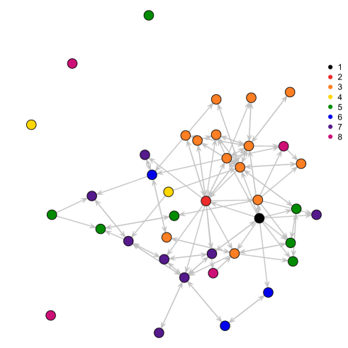
Figure 1: Kapferer Tailor Shop directed graph. Nodal covariates consists of employees’ occupational categories: 1=head tailor, 2=cutter, 3=line 1 tailor, 4=button machined, 5=line 3 tailor, 6=ironer, 7=cotton boy, 8=line 2 tailor.

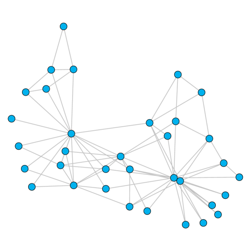
Figure 2: Zachary’s karate club undirected graph.

2 Getting Bergm

The Bergm package can be obtained and loaded in R using the following commands: R> install.packages("Bergm") R> library("Bergm") Since Bergm depends on ergm (hun:han:but:goo:mor08) (which in turn depends on network (but08)), coda (plu:bes:cow:vin06), and mvtnorm (gen12). Installing the package will automatically load all the dependencies. All of these packages are available on the Comprehensive R Archive Network (CRAN) at http://CRAN.R-project.org.

The results presented in this paper have been obtained using R version 2.15.1 on a Mac using Bergm version 2.5; ergm version 3.0-3; network version 1.7-1; coda version 0.15-2; and mvtnorm version 0.9-9993.

3 Bayesian exponential random graphs

The Bayesian approach to statistical problems is probabilistic. Inference is based on the posterior distribution which is the conditional probability of the unknown quantities given the observed ones. The posterior distribution extracts the information in the data and provide a complete summary of the uncertainty about the unknowns.

In the ERGM context (see was:pat96 and rob:pat:kal:lus07), the purpose of Bayesian inference is to learn about the posterior distribution of the model parameters $\theta$ of an observed graph $y$ on $n$ nodes:

$$p(\hbox{\boldmath$\theta$}|\hbox{\boldmath$y$})=\frac{p(\hbox{\boldmath$y$}|\hbox{\boldmath$\theta$})\;p(\hbox{\boldmath$\theta$})}{p(\hbox{\boldmath$y$})}=\frac{\exp\{\hbox{\boldmath$\theta$}^{t}s(\hbox{\boldmath$y$})\}}{z(\hbox{\boldmath$\theta$})}\;\frac{p(\hbox{\boldmath$\theta$})}{p(\hbox{\boldmath$y$})},$$ (1)

where $s(\hbox{\boldmath$y$})$ is a known vector of sufficient network statistics (Figure 3) (mor:han:hun08), $p(\hbox{\boldmath$\theta$})$ is a prior distribution placed on $\theta$, $z(\hbox{\boldmath$\theta$})$ is the likelihood normalizing constant, and $p(\hbox{\boldmath$y$})$ is the model evidence. Equation 1 provides a probabilistic statement about how likely parameter values are after observing the data $y$. The likelihood $p(\hbox{\boldmath$y$}|\hbox{\boldmath$\theta$})$ is translated into a proper probability distribution that can be summarised by computing expected values, standard deviations, quantiles, etc.

(a)

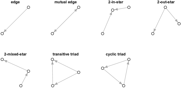
(b)

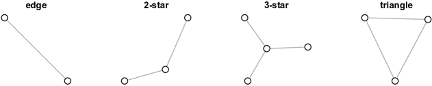
Figure 3: Some of the most used configurations for directed (a) and undirected (b) graphs.

Unfortunately the posterior distribution (Equation 1) is doubly-intractable as both $z(\hbox{\boldmath$\theta$})$ and $p(\hbox{\boldmath$y$})$ cannot be evaluated analytically (kos04). This makes the use of standard MCMC procedures infeasible.

In order to carry out Bayesian inference for ERGMs, the Bergm package makes use of a combination of Bayesian algorithms and MCMC techniques. The exchange algorithm circumvents the problem of computing the normalizing constants of the ERGM likelihoods, while the use of multiple chains interacting with each others (population MCMC approach) by means of adaptive direction sampling is able to speed up the computations and improve chain mixing quite significantly.

4 Bayesian parameter estimation

In order to approximate the posterior distribution $p(\hbox{\boldmath$\theta$}|\hbox{\boldmath$y$})$, the Bergm package uses the exchange algorithm described in Section 4.1 of cai:fri11 to sample from the following distribution:

$$p(\hbox{\boldmath$\theta$}^{\prime},\hbox{\boldmath$y$}^{\prime},\hbox{\boldmath$\theta$}|\hbox{\boldmath$y$})\propto p(\hbox{\boldmath$y$}|\hbox{\boldmath$\theta$})p(\hbox{\boldmath$\theta$})\epsilon(\hbox{\boldmath$\theta$}^{\prime}|\hbox{\boldmath$\theta$})p(\hbox{\boldmath$y$}^{\prime}|\hbox{\boldmath$\theta$}^{\prime})$$

where $p(\hbox{\boldmath$y$}^{\prime}|\hbox{\boldmath$\theta$}^{\prime})$ is the likelihood on which the simulated data $\hbox{\boldmath$y$}^{\prime}$ are defined and belongs to the same exponential family of densities as $p(\hbox{\boldmath$y$}|\hbox{\boldmath$\theta$})$, $\epsilon(\hbox{\boldmath$\theta$}^{\prime}|\hbox{\boldmath$\theta$})$ is any arbitrary proposal distribution for the augmented variable $\hbox{\boldmath$\theta$}^{\prime}$. As we will see in the next section, this proposal distribution is set to be a normal centered at $\theta$.

At each MCMC iteration, the exchange algorithm consists of a Gibbs update of $\hbox{\boldmath$\theta$}^{\prime}$ followed by a Gibbs update of $\hbox{\boldmath$y$}^{\prime}$, which is drawn from the $p(\cdot|\hbox{\boldmath$\theta$}^{\prime})$ via an MCMC algorithm (hun:han:but:goo:mor08). Then a deterministic exchange or swap from the current state $\theta$ to the proposed new parameter $\hbox{\boldmath$\theta$}^{\prime}$. This deterministic proposal is accepted with probability:

$$\min\left(1,\frac{q_{\hbox{\boldmath$\theta$}}(\hbox{\boldmath$y$}^{\prime})p(\hbox{\boldmath$\theta$}^{\prime})\epsilon(\hbox{\boldmath$\theta$}|\hbox{\boldmath$\theta$}^{\prime})q_{\hbox{\boldmath$\theta$}^{\prime}}(\hbox{\boldmath$y$})}{q_{\hbox{\boldmath$\theta$}}(\hbox{\boldmath$y$})p(\hbox{\boldmath$\theta$})\epsilon(\hbox{\boldmath$\theta$}^{\prime}|\hbox{\boldmath$\theta$})q_{\hbox{\boldmath$\theta$}^{\prime}}(\hbox{\boldmath$y$}^{\prime})}\times\frac{z(\hbox{\boldmath$\theta$})z(\hbox{\boldmath$\theta$}^{\prime})}{z(\hbox{\boldmath$\theta$})z(\hbox{\boldmath$\theta$}^{\prime})}\right),$$

where $q_{\hbox{\boldmath$\theta$}}$ and $q_{\hbox{\boldmath$\theta$}^{\prime}}$ indicates the unnormalised likelihoods with parameter $\theta$ and $\hbox{\boldmath$\theta$}^{\prime}$, respectively. Notice that all the normalising constants cancel above and below in the fraction above, in this way avoiding the need to calculate the intractable normalising constant.

The exchange algorithm is implemented by the bergm function in the following way:

$$\min\left(0,\;\left[\hbox{\boldmath$\theta$}-\hbox{\boldmath$\theta$}^{\prime}\right]^{t}\left[s(\hbox{\boldmath$y$}^{\prime})-s(\hbox{\boldmath$y$})\right]+\log\left[\frac{p(\hbox{\boldmath$\theta$}^{\prime})}{p(\hbox{\boldmath$\theta$})}\right]\right)$$

end for

4.1 Block-update sampler

Step 1 of the algorithm consists in generating $\hbox{\boldmath$\theta$}^{\prime}$ from some proposal distribution within each iteration. Bergm uses a block-update sampler with normal proposal to simultaneously update of the parameter values in the MCMC chain:

$$\epsilon(\hbox{\boldmath$\theta$}^{\prime}|\hbox{\boldmath$\theta$})\sim\mathcal{N}(\hbox{\boldmath$\theta$},\hbox{\boldmath$\Sigma$}_{\epsilon}).$$ (2)

Typically, tuning the parameter $\hbox{\boldmath$\Sigma$}_{\epsilon}$ of the proposal distribution $\epsilon$ from which $\hbox{\boldmath$\theta$}^{\prime}$ is drawn represents the crucial part of the algorithm since a poor tuning of the proposal parameter $\hbox{\boldmath$\Sigma$}_{\epsilon}$ can slow down the chain’s mixing rate and therefore the algorithm can take a very long time to converge to the stationary posterior density. By default $\hbox{\boldmath$\Sigma$}_{\epsilon}$ is set to a diagonal matrix with every diagonal entry equal to $0.0025$.

4.2 Parallel adaptive direction sampler

In order to improve mixing a parallel adaptive direction sampler (ADS) (gil:rob:geo94; rob:gil94) is considered: at the $i$-th iteration of the algorithm we have a collection of $H$ different chains interacting with one another. By construction, the state space consists of $\{\hbox{\boldmath$\theta$}_{1},\dots,\hbox{\boldmath$\theta$}_{H}\}$ with target distribution $p(\hbox{\boldmath$\theta$}_{1}|\hbox{\boldmath$y$})\otimes\dots\otimes p(\hbox{\boldmath$\theta$}_{H}|\hbox{\boldmath$y$})$. A parallel ADS move consists of generating a new value $\hbox{\boldmath$\theta$}^{\prime}_{h}$ from the difference of two parameters $\hbox{\boldmath$\theta$}_{h_{1}}$ and $\hbox{\boldmath$\theta$}_{h_{2}}$ (randomly selected from other chains) multiplied by a scalar term $\gamma$ which is called parallel ADS move factor plus a random term $\epsilon$ called parallel ADS move parameter (Figure 4) which is equivalent to the block-update sampler defined in (Equation 2). The algorithm can be summarised as follows:

$$\min\left(0,\left[\hbox{\boldmath$\theta$}_{h}-\hbox{\boldmath$\theta$}^{\prime}_{h}\right]^{t}\left[s(\hbox{\boldmath$y$}^{\prime})-s(\hbox{\boldmath$y$})\right]+\log\left[\frac{p(\hbox{\boldmath$\theta$}^{\prime}_{h})}{p(\hbox{\boldmath$\theta$}_{h})}\right]\right)$$

end for
end for

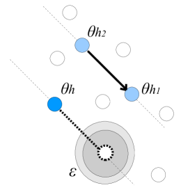
Figure 4: The parallel ADS move of the current state (darker blue dot) consists of generating a new parameter value along the direction made by the difference of two randomly sampled parameter states (light blue dots) belonging to different chains plus a random term.

4.3 Kapferer tailor shop network

Consider the Kapferer Tailor Shop network and a 3-dimensional model including the following network statistics: edges (edges), mutual edges (mutual) and cyclic triples (ctriple) involving nodes with the same job status, where the job status is represented by a categorical nodal attribute variable consisting of 8 levels described in Figure 1.

edges	$\sum_{i\neq j}y_{ij}$
mutual	$\sum_{i\neq j}y_{ij}y_{ji}$
ctriple("job")	$\sum_{i\neq j\neq k}y_{ij}y_{jk}y_{ki}$ where $i,j,k$ have the same job status

The format of the model specification is the same of an ergm formula: R> formula <- y   edges + mutual + ctriple("job") Then we can use the bergm function to sample from the posterior distribution using the MCMC algorithm described above. In this example we use the parallel ADS procedure described in Section 4.2. By default, the number of chains in the population is set as twice the number of dimensions of the model. It is possible to choose a different number of chains by using the argument nchains. In order to perform the block-site update described in Section 4.1 it is necessary to set nchains = 1. For each chain, we can then set the number of burn-in iterations (burn.in) and the number of iterations after the burn-in (main.iters). The number of iterations used to simulate a network $\hbox{\boldmath$y$}^{\prime}$ at each iteration is defined by the argument aux.iters. R> post.est <- bergm(formula, + burn.in=500, + gamma=0.7, + main.iters=1500, + aux.iters=25000) The population MCMC with parallel ADS move is the default procedure of the bergm function. The total number of iterations, e.g., the size of the posterior sample, is nchains $\times$ main.iters. The proposal covariance structure $\hbox{\boldmath$\Sigma$}_{\epsilon}$ is defined by the argument sigma.epsilon which is set to be a diagonal matrix with every diagonal entry equal to a small number. In many cases, good mixing of the chain is ensured by a sensible tuning of the parallel ADS move factor gamma and therefore the argument sigma.epsilon can be generally left at its default value. The parameter gamma can be easily tuned to achieve a suitable acceptance rate by starting from its default value ($0.5$). Empirically it has been observed that the value of gamma can range from $0.1$ to $1.5$ depending on the size of network and the kind of network statistics included in the model.

As said above, parallel ADS is adopted as the default procedure but it is automatically disabled in the case of uni-dimensional models where the block-update sampler is used and the argument gamma is used to tune the variance of the normal proposal distribution $\epsilon$.

After completing the estimation, post.est is an object of the class bergm and contains a list of attributes among which are the real and CPU time (in seconds) taken by the estimation process: R> post.est$time\CodeOutput usersystemelapsed153.5521.097156.154ItispossibletovisualisetheresultsoftheMCMCestimationbyusingthe\code{bergm.output}functionwhichisbasedonthe\pkg{coda}package\cite[citep]{(\@@bibref{AuthorsPhrase1Year}{plu:bes:cow:vin06}{\@@citephrase{, }}{})}whichisan\proglang{R}packageforMCMCoutputanalysisanddiagnostics.\CodeChunk\CodeInput R>bergm.output(post.est,lag.max=50)\CodeOutput MCMCresultsforModel:y~{}edges+mutual+ctriple("job")\par Posteriormean:theta1(edges)theta2(mutual)theta3(ctriple.job)Chain1-3.40788063.79659930.8307185Chain2-3.32286453.64956620.8075557Chain3-3.40089493.80346150.8032079Chain4-3.42203183.82764770.7884897Chain5-3.42116733.79608810.8026476Chain6-3.45663673.87620170.8350634\par Posteriorsd:theta1(edges)theta2(mutual)theta3(ctriple.job)Chain10.32884980.58536080.1848051Chain20.27208090.47398550.1782770Chain30.26069940.49391380.1875215Chain40.25305380.48270110.1817614Chain50.27314120.49978580.1635572Chain60.25067240.47093640.1691319\par Acceptancerate:Chain10.2713333Chain20.2340000Chain30.2393333Chain40.2280000Chain50.2240000Chain60.2353333\par\par Overallposteriordensityestimate:theta1(edges)theta2(mutual)theta3(ctriple.job)Post.mean-3.40524603.79159410.8112805Post.sd0.27729420.50724830.1784213\par Overallacceptancerate:0.238666666666667\par TheoutputaboveshowstheresultsoftheMCMCestimation:posteriormeansandstandarddeviations,andacceptanceratesforeverychaininthepopulationandfortheoverallchain.Noticethattheposteriorsummariesofeachchainareconsistentwitheachother.Figure~{}\ref{fig:mcmcout}displaystheMCMCdiagnosticplotsproducedbythe\code{bergm.output}function.Inthisexample,weobservealowdensityeffectexpressedbythenegativevalueoftheposteriormeanoftheedgeeffectparameter($θ_1$)combinedwiththepositivemutualityandtransitivitywithinpeoplehavingthesamejobstatusexpressedbythemutualedgeparameter($θ_2$)andcyclictripleparameter($θ_3$)respectively.Theoverallacceptancerateisaround$24%$andtheautocorrelationisnegligibleafterlag50.\text{Figure 5Figure 55Figure 55MCMCdiagnosticsfortheoverallchain.The3plotcolumns,fromlefttoright,are}$