Self-isospectral tri-supersymmetry in ${\cal PT}$-symmetric quantum systems with pure imaginary periodicity

Abstract

We study a reflectionless $\mathcal{PT}$-symmetric quantum system described by the pair of complexified Scarf II potentials mutually displaced in the half of their pure imaginary period. Analyzing the rich set of intertwining discrete symmetries of the pair, we find an exotic supersymmetric structure based on three matrix differential operators that encode all the properties of the system, including its reflectionless (finite-gap) nature. The structure we revealed particularly sheds new light on the splitting of the discrete states into two families, related to the bound and resonance states in Hermitian Scarf II counterpart systems, on which two different series of irreducible representations of $sl(2,\mathbb{C})$ are realized.

Keywords: Supersymmetric quantum mechanics; ${\cal PT}$-symmetry; non-Hermitian Hamiltonians; self-isospectrality; finite-gap systems; non-linear supersymmetry.

1 Introduction

Fourteen years ago, Bender and Boettcher discovered a huge and remarkable class of non-Hermitian quantum Hamiltonians which exhibit an entirely real spectrum [1]. One of the key points of the observation was the requirement of a $\mathcal{PT}$-symmetry generated by the product of the parity, ${\cal P}$, and time, ${\cal T}$, inversion operators,

$${\cal P}\,x\,{\cal P}=-x,\qquad{\cal T}\,x\,{\cal T}=x,\quad{\cal T}\,i\,{\cal T}=-i\,,$$ (1.1)

that substitutes the usual quantum mechanical property of Hermiticity. This condition, however, is necessary but not sufficient for the reality of the spectrum; it is also required that eigenfunctions of a ${\cal PT}$-symmetric Hamiltonian must be simultaneously eigenfunctions of the $\mathcal{PT}$ operator. In this case we say that the ${\cal PT}$ symmetry is unbroken, otherwise the eigenvalues are not real, a part or all of them appear in complex conjugate pairs, and the ${\cal PT}$ symmetry is broken [1, 2, 3].

Nowadays, quantum mechanics with non-Hermitian Hamiltonians transformed into an independent line of research where, specifically, the notion of the ${\cal PT}$-symmetry was generalized into the condition of pseudo-Hermiticity [4]. Non-Hermitian Hamiltonians appear in physics in diverse areas including quantum optics, cosmology, atomic and condensed matter physics, magnetohydrodynamics, among others. For a good review of the developments in the area and applications, see [5, 6] and references therein.

On the other hand, there is a wide class of modern techniques and methods which prove their effectiveness in the study of quantum mechanical systems. One of them is supersymmetric quantum mechanics (SUSYQM), introduced initially by Witten as a toy model to study the spontaneous supersymmetry breaking [7]. Over the past few decades, SUSYQM transformed into a powerful tool in quantum physics [8] which turns out to be useful, for example, in the spectral analysis as well as in searching for new solvable systems. SUSYQM in its usual form is based on a Darboux transformation that relates two Hamiltonians by means of an intertwining, linear differential operator, and leads, as a result, to a complete or almost complete isospectrality of both systems [9].

The concept of Darboux transformations and SUSYQM was generalized in different aspects that lead to the discovery of the classes of quantum systems that reveal non-linear [10, 11, 12], bosonized [11, 13, 14, 15] and self-isospectral [16, 17, 18, 19, 20] supersymmetries. Particularly, a certain class of potentials was found in which all the mentioned specific types of supersymmetries were brought to light in a form of a peculiar structure that was coined in [20] as “tri-supersymmetry”. Such a structure was shown to underlie special properties of some physical quantum systems [21, 22, 23, 24, 25]. Among the principal characteristics of tri-supersymmetry, which will be described below, is the existence of three integrals of motion in the form of supercharges which encode the main properties of the corresponding systems. An example of the systems that reveal a tri-supersymmetric structure is provided by the Hermitian finite-gap periodic potentials [20], which in the limit when their real period tends to infinity are known as reflectionless potentials.

The idea of supersymmetry in some of its versions was adapted in the context of non-Hermitian Hamiltonians [26, 27, 28, 29, 30, 31, 32, 33]. Although the non-linear and self-isospectral supersymmetries were studied before in the systems with non-Hermitian Hamiltonians [34], the presence in them of a supersymmetric structure that would unify the mentioned types of supersymmetry remains to be unknown. One can wonder therefore if there exist non-Hermitian potentials of finite-gap nature that display the properties to be similar to those of the Hermitian counterpart, and what are the peculiarities of the associated supersymmetric structure.

The purpose of the present article is to report the observation of an exotic tri-supersymmetric structure in a broad class of ${\cal PT}$-symmetric extended finite-gap systems. This allows us, on the one hand, to understand and explain the main features of their spectra by analyzing the properties of the supercharges; on the other hand, we explicitly trace out the differences that appear in comparison with the Hermitian case, at the level of potentials as well as in the generic properties of tri-supersymmetry. The importance of a hidden, pure imaginary period in non-periodic on a real line finite-gap systems is clarified, particularly, in the light of tri-supersymmetric structure. We achieve all this by considering the pairs of ${\cal PT}$-symmetric complexified Scarf II potentials mutually displaced in the half of their unique imaginary period. For special values of the parameters these potentials become perfectly transparent, i.e. reflectionless. It is exactly for such special parameter values the tri-supersymmetric structure arises and allows us to clarify its nontrivial interplay with various discrete symmetries of the potentials. The supersymmetric structure we reveal gives us a new insight on the splitting of discrete states in such a class of $\mathcal{PT}$-symmetric quantum systems into two distinct families, on which two different representations of the $sl(2,\mathbb{C})$ algebra are realized, the fact that was established initially by Bagchi and Quesne by using group theoretical methods [35]. Note here that the complexified Scarf II potential was extensively studied in the literature in the context of ${\cal PT}$-symmetric and pseudo-Hermitian Hamiltonians; the updated summary on these investigations can be found in ref. [36]. Recently, this potential also attracted the attention in different areas of physics such as quantum field theory in curved spacetimes [37], soliton theory in nonlinear integrable systems [38] and also the physics of optical solitons [39].

The plan of the article is as follows. In sections 2 and 3 the basic properties of the pair of complexified mutually conjugated Scarf II potentials are reviewed. Specifically, in the next section we study various discrete symmetries of the potentials, describe spectral properties of the systems in dependence on the parameter values, and describe the relation with the other known potentials. In section 3 we first present the explicit expressions for the two families of the singlet states in the spectrum, and then discuss the continuous spectrum and its relation with that of the free particle by means of Darboux-Crum transformations that underlie the non-linear supersymmetry. The tri-supersymmetric structure is described in section 4. Section 5 provides two concrete nontrivial examples of the systems with two and three bound states to illustrate the general results. In section 6 we present the discussion and concluding remarks.

2 Discrete symmetries and relations

Consider a pair of complexified Scarf II potentials

$$V_{l,m}^{\pm}(x)=-\frac{l^{2}+m(m+1)}{\cosh^{2}x}\pm il(2m+1)\frac{\sinh x}{\cosh^{2}x}\,\,.$$ (2.1)

We suppose that $l$ and $m$ are real parameters, and $x\in\mathbb{R}$. Potentials (2.1) are then free of singularities on the real line, and their real and imaginary parts vanish for $x\rightarrow\pm\infty$, see Fig. 1.

Figure 1: Plot of real and imaginary parts of the complexified Scarf II potential $V^{+}_{1,1}$, which here as well as in a generic case of (2.1) are even and odd functions, respectively.

Pair (2.1) can be transformed into a pair of original, real Scarf II potentials [40] by a substitution $l\rightarrow il$, see Fig. 2.

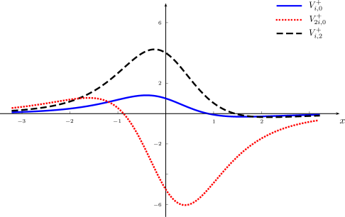
Figure 2: Examples of original (real) Scarf II potentials.

Both the original and complexified potentials have a pure imaginary period $2i\pi$.

Parity inversion, ${\cal P}$, and time reversal, ${\cal T}$, operators intertwine the completely isospectral potentials (2.1),

$${\cal P}V_{l,m}^{\pm}=V_{l,m}^{\mp}{\cal P},\qquad{\cal T}V_{l,m}^{\pm}=V_{l,m}^{\mp}{\cal T}.$$ (2.2)

As $V^{\pm}_{-l,m}=V^{\pm}_{l,-m-1}=V^{\mp}_{l,m}$, another pair of intertwiners is provided by operators $\mathcal{R}_{l}$ and $\mathcal{R}_{m}$, which act on the parameters $l$ and $m$, $\mathcal{R}_{l}:\,(l,m)\rightarrow(-l,m)$, $\mathcal{R}_{m}:(l,m)\rightarrow(l,-m-1)$,

$$\mathcal{R}_{l}V_{l,m}^{\pm}=V_{l,m}^{\mp}\mathcal{R}_{l},\qquad\mathcal{R}_{m}V_{l,m}^{\pm}=V_{l,m}^{\mp}\mathcal{R}_{m}\,.$$ (2.3)

Yet another pair of intertwining operators is given by pure imaginary translations for the half of the period $2i\pi$, $T_{+}:\ x\rightarrow x+i\pi$ and $T_{-}:\ x\rightarrow x-i\pi$,

$$T_{+}V_{l,m}^{\pm}=V_{l,m}^{\mp}T_{+},\qquad T_{-}V_{l,m}^{\pm}=V_{l,m}^{\mp}T_{-}\,.$$ (2.4)

The product of any two of the listed intertwining operators, except of $T_{+}=\exp(\pi\frac{d}{dx})$ and $T_{-}=\exp(-\pi\frac{d}{dx})$, $T_{+}T_{-}=1$, is a nontrivial discrete symmetry of each of potentials (2.1). Particularly, we find that each potential of the pair is ${\cal PT}$-symmetric,

$$[{\cal PT},V_{l,m}^{\pm}]=0\,.$$ (2.5)

The potentials satisfy also the relation

$$V_{l,m}^{\pm}=V_{-l,-m-1}^{\pm}\,,$$ (2.6)

which is produced by a composition $\mathcal{R}_{l}\mathcal{R}_{m}$ of the intertwining generators (2.3).

We also have a symmetry relation

$$V_{l,m}^{\pm}=V_{m+\frac{1}{2},\,l-\frac{1}{2}}^{\pm}\,,$$ (2.7)

that will play a key role in the analysis below. The composition of (2.6) and (2.7) produces yet another symmetry

$$V_{l,m}^{\pm}=V_{-m-\frac{1}{2},-l-\frac{1}{2}}^{\pm}\,\,.$$ (2.8)

The nature of relations (2.3) and (2.6)–(2.8) takes a somewhat more transparent form if to redefine the parameters [41]: $(l,m)\rightarrow(\alpha_{+},\alpha_{-}$), $\alpha_{\pm}=m\pm l+\frac{1}{2}$. Then the coefficients in (2.1) are transformed into $l^{2}+m(m+1)=\frac{1}{2}[\alpha_{+}^{2}+\alpha_{-}^{2}-\frac{1}{2}]$ and $l(2m+1)=\frac{1}{2}(\alpha_{+}^{2}-\alpha_{-}^{2})$, and symmetry (2.7) corresponds to a reflection $\mathcal{P}_{\alpha_{-}}:\,(\alpha_{+},\alpha_{-})\rightarrow(\alpha_{+},-\alpha_{-})$ in the plane of $\alpha$-parameters. Intertwining relations (2.3) are given by the products of reflection $\mathcal{P}_{\alpha_{-}}$ and $\alpha$-rotations for $\pm\pi/2$, $\mathcal{R}_{+\pi/2}:\,(\alpha_{+},\alpha_{-})\rightarrow(\alpha_{-},-\alpha_{+})$ and $\mathcal{R}_{-\pi/2}:\,(\alpha_{+},\alpha_{-})\rightarrow(-\alpha_{-},\alpha_{+})$, $\mathcal{R}_{l}=\mathcal{P}_{\alpha_{-}}\mathcal{R}_{+\pi/2}$, $\mathcal{R}_{m}=\mathcal{P}_{\alpha_{-}}\mathcal{R}_{-\pi/2}$, while symmetries (2.6) and (2.8) correspond, respectively, to a $\pi$-rotation $(\alpha_{+},\alpha_{-})\rightarrow(-\alpha_{+},-\alpha_{-})$ and to a reflection in $\alpha_{+}$, $\mathcal{P}_{\alpha_{+}}:\,(\alpha_{+},\alpha_{-})\rightarrow(-\alpha_{+},\alpha_{-})$.

It will be more convenient for us, however, to work in terms of the parameters $l$ and $m$. Relations (2.6)–(2.8) allow us to interchange integer values with half-integer ones as well as positive with negative values. By this reason, without loss of generality we can suppose that $l$ and $m$ are non-negative integers; sometimes, however, negative and half-integer values will be important as well.

The described discrete relations and symmetries form the base for a rich exotic supersymmetric structure that we will reveal in the extended system ${\cal H}_{l,m}=diag(H^{+}_{l,m},H^{-}_{l,m})$,

$$H^{\pm}_{l,m}=-\frac{d^{2}}{dx^{2}}+V_{l,m}^{\pm}\,,$$ (2.9)

with pseudo-Hermitian Hamiltonians [4],

$$H^{\pm}_{l,m}={\cal P}(H^{\pm}_{l,m})^{\dagger}\,{\cal P}\,,$$ (2.10)

where we have taken into account the relation ${\cal P}^{-1}={\cal P}$.

The spectra of $H^{\pm}_{l,m}$ display different features in dependence on the values of the parameters $l$ and $m$. The eigenfunctions of Hamiltonians (2.9) may or may not be simultaneous eigenstates of the ${\cal PT}$ operator. The situation is known as unbroken ${\cal PT}$ symmetry in the former case, or spontaneously broken in the latter case. As was shown in [1, 2, 3], the spectrum of a ${\cal PT}$ symmetric Hamiltonian is real when its eigenfunctions are simultaneously the eigenstates of the ${\cal PT}$ operator. In the case of the $H^{\pm}_{l,m}$, this situation holds when

$$l^{2}+\left(m+1/2\right)^{2}\geq|2l\left(m+1/2\right)|\,,$$ (2.11)

that is always valid for real $l$ and $m$ [42]. For real $l$ and $m$, the spectra of $H^{+}_{l,m}$ and $H^{-}_{l,m}$ have a finite number of bound states of non-degenerate energies, while the probability flux is conserved in a scattering sector. It was pointed out in [43] that an imaginary displacement in the spatial coordinate $x\rightarrow x+i\delta$, where $\delta\in\mathbb{R}$, breaks in general the conservation of probability, i.e. $|T|^{2}+|R|^{2}\neq 1$. There is, however, a case that shows several special properties for this class of shifted potentials. When $l$ and $m$ take simultaneously non-negative integer values, the reflection coefficient vanishes, $|R|=0$, and the probability is conserved independently of any displacement $\delta\neq\pm\pi/2$, see below. As a result potentials (2.1) belong to the class of reflectionless potentials [44]. In this case both potentials have the same spectrum with $m+l+1$ singlet states, where $m+l$ of them are bound states of negative energies, and there is a singlet state of zero energy at the bottom of the continuous part of the spectrum. We discuss the spectral characteristics of (2.9) in more details in Section 3.

Within a framework of $\mathcal{PT}$-symmetric quantum mechanics [5], or in a more general framework of the systems with pseudo-Hermitian Hamiltonians [6], it was shown that the $\mathcal{PT}$ integral can be supplied with yet another nontrivial (nonlocal) integral of motion that has a nature of the charge conjugation operator, $\mathcal{C}$ [45]. This allows finally to define a positive definite scalar product to extend a probabilistic interpretation for the case of $\mathcal{PT}$-symmetric systems. Here, we just have in mind this general picture when discuss the bound and scattering states by referring to original papers on the subject.

The double degeneracy in the spectrum for the scattering sector together with the reflectionless property and the finite number of singlet states indicate that each system $H^{+}_{l,m}$ and $H^{-}_{l,m}$ possesses a hidden, bosonized non-linear supersymmetry [11, 13] as this happens for Hermitian reflectionless Hamiltonians [14, 20]. In fact for integer values of $l$ and $m$, potentials (2.1) are solutions of the KdV hierarchy: they satisfy the stationary $s$-KdV_n, $n=l+m$, non-linear equations [46]. This means that there should exist non-trivial integrals of motion ${\mathbb{A}}^{+}_{2n+1}$ and ${\mathbb{A}}^{-}_{2n+1}$ for Hamiltonians (2.9) in the form of differential operators of order $2n+1$. These integrals should satisfy relations

$$[{\mathbb{A}}^{+}_{2n+1},H^{+}_{l,m}]=[{\mathbb{A}}^{-}_{2n+1},H^{-}_{l,m}]=0,\qquad({\mathbb{A}}^{\pm}_{2n+1})^{2}=P(H^{\pm}_{l,m}),\qquad n=l+m\,,$$ (2.12)

where $P(H^{\pm}_{l,m})$ is a polynomial of order $2n+1$, i.e. ${\mathbb{A}}^{+}_{2n+1}$ and $H^{+}_{l,m}$, as well as ${\mathbb{A}}^{-}_{2n+1}$ and $H^{-}_{l,m}$, should compose a Lax pair [47, 48].

There are particular cases for which $H^{\pm}_{l,m}$ are completely isospectral to the reflectionless Pöschl-Teller Hamiltonians [49]

$$H^{PT}_{\lambda}=-\frac{d^{2}}{dx^{2}}-\frac{\lambda(\lambda+1)}{\cosh^{2}x},\qquad\lambda\in\mathbb{Z}\,.$$ (2.13)

Namely, the Pöschl-Teller and the complexified Scarf II potentials are related by a transformation of an imaginary displacement and a rescaling of the variable,

$$H^{PT}_{\lambda}(x\pm i\pi/4)=4H^{\pm}_{l,m}(2x)\,,\quad\text{for}\quad\left\{\begin{array}[]{ccc}m=l-1,\quad\quad\lambda=m+1\,,\\ \text{and}\\ m=l,\quad\quad\lambda=m\,.\end{array}\right.$$ (2.14)

Another interesting relation is with a generalized, singular Pöschl-Teller potential [8]

$$V_{l,m}^{GPT}(x)=\frac{l^{2}+m(m+1)}{\sinh^{2}x}+l(2m+1)\frac{\cosh x}{\sinh^{2}x}\,.$$ (2.15)

The singularity can be removed by complex shifting [35]. For special values of such a shifting we get the ${\cal PT}$-symmetric pair of potentials (2.1),

$$V_{l,m}^{GPT}(x\pm i\pi/2)=V_{l,m}^{\pm}(x)\,.$$ (2.16)

It is worth to note that the potentials (2.1) and corresponding Hamiltonians admit a representation that generalizes Eq. (2.14),

$$H_{l,m}^{+}=\frac{1}{4}\left(-\frac{d^{2}}{d\xi^{2}}-\frac{r(r+1)}{\cosh^{2}\xi}-\frac{s(s+1)}{\cosh^{2}(\xi+i\frac{\pi}{2})}\right)\,,$$ (2.17)

$$H_{l,m}^{-}=\frac{1}{4}\left(-\frac{d^{2}}{d\xi^{2}}-\frac{s(s+1)}{\cosh^{2}\xi}-\frac{r(r+1)}{\cosh^{2}(\xi+i\frac{\pi}{2})}\right)\,,$$ (2.18)

where $\xi=\frac{x}{2}+i\frac{\pi}{4}$, and

$$r=l+m,\qquad s=l-m-1\,.$$ (2.19)

Representations (2.17) and (2.18) correspond, on the one hand, to the relation (2.4) between potentials (2.1) generated by the shift in the half of their imaginary period,

$$H_{l,m}^{-}(\xi)=H_{l,m}^{+}\left(\xi+i\frac{\pi}{2}\right)\,.$$ (2.20)

On the other hand, the generators of intertwining relations (2.3) correspond here to $\mathcal{R}_{l}:\,(r,s)\rightarrow(-s-1,-r-1)$ and $\mathcal{R}_{m}:\,(r,s)\rightarrow(s,r)$.

We will return to (2.20) in the discussion of the supersymmetric structure, but here we note that in the context of periodic (elliptic) finite-gap potentials, a so called tri-supersymmetry appears when the superpartner potentials are the associated Lamé potentials shifted mutually in the half of the real period [20]. As we will show below, the extended system ${\cal H}_{l,m}$ constructed from (2.9) also possesses a tri-supersymmetry in which the imaginary period, the ${\cal PT}$- symmetry, the discrete symmetries (2.6) and (2.8), and the non-linear supersymmetry together play a fundamental role to form altogether a unified structure.

As a final comment on relation of (2.1) with periodic finite-gap potentials, we note that there is a generalization of the family of the associated Lamé potentials known as the Darboux-Treibich-Verdier potentials [51]. In terms of the (double periodic) Jacobi elliptic functions they read

$$V^{DTV} = n_{1}(n_{1}+1)k^{2}\mathrm{sn}^{2}x+n_{2}(n_{2}+1)k^{2}\mathrm{sn}^{2}(x+iK^{\prime})$$

$$+ n_{3}(n_{3}+1)k^{2}\mathrm{sn}^{2}(x+K+iK^{\prime})+n_{4}(n_{4}+1)k^{2}\mathrm{sn}^{2}(x+K)$$

$$= n_{1}(n_{1}+1)k^{2}\mathrm{sn}^{2}x+n_{2}(n_{2}+1)\frac{1}{\mathrm{sn}^{2}x}+n_{3}(n_{3}+1)\frac{\mathrm{dn}^{2}x}{\mathrm{cn}^{2}x}+n_{4}(n_{4}+1)\frac{k^{2}\mathrm{cn}^{2}x}{\mathrm{dn}^{2}x}\,.$$

Here $0<k<1$ is the modular parameter, and (2) has a real, $2K$, and an imaginary, $2iK^{\prime}$, periods; $K=K(k)$ is the elliptic complete integral of the first kind and $K^{\prime}=K(k^{\prime})$, $k^{\prime}=\sqrt{1-k^{2}}$ [53]. The finite-gap nature of (2) appears when parameters $n_{i}$ take integer values. Particularly, when $n_{2}=n_{3}=0$, potential (2) reduces to the finite-gap associated Lamé potential [20, 52]. When the modular parameter takes the limit $k\rightarrow 1$, the real period tends to infinity, $2K\rightarrow\infty$, while $2iK^{\prime}\rightarrow i\pi$, and the potential transforms into

$$V^{DTV}\xrightarrow[k\rightarrow{}1]{\,}-\frac{n_{1}(n_{1}+1)}{\cosh^{2}x}-\frac{n_{2}(n_{2}+1)}{\cosh^{2}(x+i\frac{\pi}{2})}+const\,,$$ (2.22)

that has the form of potentials (2.17) and (2.18).

In the next section we will study the states of the ${\cal PT}$-symmetric systems $H^{\pm}_{lm}$ in the light of the discrete symmetries and relations that we have discussed.

3 Wavefunctions and differential intertwiners

The group theoretical methods and supersymmetry are the powerful tools in the study of quantum mechanical systems. The Hamiltonians (2.9) provide a good example of the systems for which these techniques work effectively, particularly, to analyze the spectrum and eigenfunctions. In this direction, using irreducible representations of the $sl(2,\mathbb{C})$ algebra, it was found in [35] that the non-degenerate parts of the spectra of potentials (2.1) are described by the two sets of eigenfunctions, one of which is

$$\Psi^{\pm}_{n,m}={\rm sech}^{m}\,x\,\,\exp{[\mp il\arctan(\sinh x)]}P_{n}^{l-m-1/2,-l-m-1/2}(\pm i\sinh x)\,,$$ (3.1)

where $P_{n}^{\,\alpha,\,\beta}(x)$ are the Jacobi polynomials [53]. The corresponding energy levels and the values of the parameter $n$ are

$$E_{n,m}=-(m-n)^{2},\quad n=0,1,2...\leq m\,.$$ (3.2)

The eigenfunctions $\Psi^{\pm}_{n,m}$ for $n<m$ describe $m$ bound states, while $n=m$ corresponds to the singlet zero energy state at the bottom of the continuous spectrum. With the discrete symmetry (2.7) of the potentials, $V_{l,m}^{\pm}=V_{m+\frac{1}{2},l-\frac{1}{2}}^{\pm}$, to which corresponds a transformation

$$(l,m)\rightarrow\left(m+\frac{1}{2},l-\frac{1}{2}\right)\,,$$ (3.3)

it is possible to write down the another set of the bound states,

$$\Psi^{\pm}_{n,l}={\rm sech}^{l-1/2}\,x\,\,\exp{[\mp i(m+1/2)\arctan(\sinh x)]}P_{n}^{m+1/2-l,-m-1/2-l}(\pm i\sinh x)\,,$$ (3.4)

with energies

$$E_{n,l}=-(l-n-1/2)^{2},\quad n=0,1,2...<l-1/2\,,$$ (3.5)

so that (3.1) and (3.4) represent together the $l+m+1$ singlet states of the systems (2.9).

As we will see, the separation of singlet states of each subsystem $H^{+}_{l,m}$ and $H^{-}_{l,m}$ into the two subsets is reflected by a specific nonlinear supersymmetry of the extended system $\mathcal{H}_{l,m}$. This supersymmetry is related to the (imaginary here) mutual half-period shift of the subsystems. To the best of our knowledge a similar kind of supersymmetric structure, that we shall discuss in the next section, was discussed till the moment only for finite-gap systems with Hermitian Hamiltonians [20]. To explain this structure and its origin, we present below some further comments on the properties of the Hamiltonians (2.9) and their eigenfunctions.

States (3.1) and (3.4) can also be obtained from a supersymmetry approach, by means of the Darboux-Crum transformations (for details we refer to [9]), so that it is possible to link the Hamiltonians with different values of $l$ and $m$ between them. Particularly, it is possible to relate the free particle, for which $H^{\pm}_{0,0}=-\frac{d^{2}}{dx^{2}}\equiv H_{0}$, with the generic case $H^{\pm}_{l,m}$. Note that the free particle system is presented equivalently here also by $H^{\pm}_{0,-1}$, $H^{\pm}_{1/2,-1/2}$ and $H^{\pm}_{-1/2,-1/2}$. The bound states described above can be computed from the appropriate non-physical states of the free particle, whereas the states from the continuous part of the spectrum are obtained from the plane wave states of the free system. To illustrate this picture we will show how the scattering sector of $H_{l,m}^{+}$ can be obtained having in mind that all the results for $H_{l,m}^{-}$ can be reproduced then with the help of symmetries (2.2), or by the shift for the half of the imaginary period. The construction of the bound states from the non-physical states of the free particle will be illustrated in Section 5.

Let us define the first order differential operators

$$A_{l,m}^{\pm}=\frac{d}{dx}\pm\left[\left(l-\frac{1}{2}\right)\tanh x+i\left(m+\frac{1}{2}\right){\rm sech}\,x\right]\,.$$ (3.6)

They generate the intertwining relations

$$A_{l,m}^{+}H_{l,m}^{+}=H_{l-1,m}^{+}A_{l,m}^{+}\,,\qquad A_{l,m}^{-}H_{l-1,m}^{+}=H_{l,m}^{+}A_{l,m}^{-}\,.$$ (3.7)

Now, by applying, as in the singlet states case, the discrete symmetry (3.3) to (3.6), we obtain the operators

$$B_{l,m}^{\pm}=\frac{d}{dx}\pm\left(m\tanh x+il\,{\rm sech}\,x\right)\,.$$ (3.8)

Application of symmetry (3.3) to (3.7) results then in the intertwining relations

$$B_{l,m}^{+}H_{l,m}^{+}=H_{l,m-1}^{+}B_{l,m}^{+}\,,\qquad B_{l,m}^{-}H_{l,m-1}^{+}=H_{l,m}^{+}B_{l,m}^{-}\,.$$ (3.9)

The operators $A_{l,m}^{\pm}$ are related between themselves by $A_{l,m}^{\pm}={\cal P}(A_{l,m}^{\mp})^{\dagger}{\cal P}^{-1}$. Similarly, for the operators $B_{l,m}^{\pm}$ we have $B_{l,m}^{\pm}={\cal P}(B_{l,m}^{\mp})^{\dagger}{\cal P}^{-1}$. Such relations of conjugation underly the pseudo-supersymmetry discussed in the literature for non-Hermitian systems [33], particularly, a ${\cal PT}$-symmetric one.

Coherently with the discrete symmetry (3.3), operators (3.6) and (3.8) allow us to factorize, up to an additive constant term, the same Hamiltonian in two different ways [55],

$$H_{l,m}^{+}=-A_{l,m}^{-}A_{l,m}^{+}-\left(l-\frac{1}{2}\right)^{2}=-B_{l,m}^{-}B_{l,m}^{+}-m^{2}\,.$$ (3.10)

Since $A_{l,m}^{\pm}$ as well as $B_{l,m}^{\pm}$ are $\mathcal{PT}$-antisymmetric ($\mathcal{PT}$-odd), $\{\mathcal{PT},A_{l,m}^{\pm}\}=\{\mathcal{PT},B_{l,m}^{\pm}\}=0$, the Hamiltonians $H_{l,m}^{\pm}$ are the $\mathcal{PT}$-symmetric ($\mathcal{PT}$-even) operators.

In the next section we will see further implications of existence of these two related types of factorization operators. For the moment, it is worth to note that the action of the operators $A_{l,m}^{\pm}$ and $B_{l,m}^{\pm}$ on the two-parametric family of Hamiltonians (2.9) is quite simple: while the former act by lowering and raising the parameter $l$, the latter play the same role for $m$. Using this fact, we are able now to connect, for any $l$ and $m$, the Hamiltonian $H_{l,m}^{+}$ with the free particle Hamiltonian $H_{0}$ in two different ways by making use of the operators

$${\cal D}_{l,m}^{-} = B_{l,m}^{-}B_{l,m-1}^{-}\ldots B_{l,2}^{-}B_{l,1}^{-}A_{l,0}^{-}A_{l-1,0}^{-}\ldots A_{2,0}^{-}A_{1,0}^{-}\,,$$ (3.11)

$$\tilde{{\cal D}}_{l,m}^{-} = B_{-l,-m}^{+}B_{-l,-m+1}^{+}\ldots B_{-l,-1}^{+}B_{-l,0}^{+}A_{-l+1,0}^{+}A_{-l+2,0}^{+}\ldots A_{-1,0}^{+}A_{0,0}^{+}\,.$$ (3.12)

The differential operator ${\cal D}_{l,m}^{-}$ has here the order $m+l$, meanwhile $\tilde{\cal D}_{l,m}^{-}$ has the order $m+l+1$. These operators intertwine Hamiltonian $H^{+}_{l,m}$ with the free particle Hamiltonian,

$${\cal D}_{l,m}^{-}H_{0}=H_{l,m}^{+}{\cal D}_{l,m}^{-}\,,\qquad\tilde{{\cal D}}_{l,m}^{-}H_{0}=H_{l,m}^{+}\tilde{{\cal D}}_{l,m}^{-}\,.$$ (3.13)

From (3.13) the inverse intertwining relations are easily obtained by defining ${\cal D}_{l,m}^{+}={\cal P}({\cal D}_{l,m}^{-})^{\dagger}{\cal P}^{-1}$ and $\tilde{{\cal D}}_{l,m}^{+}=-{\cal P}(\tilde{{\cal D}}_{l,m}^{-})^{\dagger}{\cal P}^{-1}$, that yields

$${\cal D}_{l,m}^{+}H_{l,m}^{+}=H_{0}{\cal D}_{l,m}^{+}\,,\qquad\tilde{{\cal D}}_{l,m}^{+}H_{l,m}^{+}=H_{0}\tilde{{\cal D}}_{l,m}^{+}\,.$$ (3.14)

Several comments are in order here. First we note that the difference of orders of the two intertwining operators (3.11) and of their conjugate ones are related to the fact that the system $H^{+}_{l,m}$ can be presented alternatively by the equivalent Hamiltonian $H^{+}_{l,-m-1}$. Another point is worth to note is that since operators $A_{l,m}^{\pm}$ and $B_{l,m}^{\pm}$ do not commute, and the path that connects the points $(l,m)$ and $(0,0)$ in the parameter plane can be chosen in different ways, the corresponding intertwining operators have not a unique form. It is the operators ${\cal D}_{l,m}^{\pm}$ and $\tilde{\cal D}_{l,m}^{\pm}$ that together with the corresponding pair of Hamiltonians $H^{\pm}_{l,m}$ will form a basis for the construction of the tri-supersymmetric structure in the present $\mathcal{PT}$-symmetric case, see Figure 3.

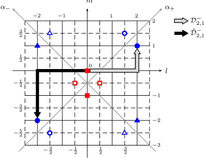
Figure 3: The family of complexified reflectionless Scarf II systems may be presented on integer or half-integer lattices in the $(l,m)$ parameters plane [in axes $\alpha_{\pm}=m\pm l+\frac{1}{2}$, the lattices for $H^{\pm}_{l,m}$ have half-integer coordinates]. Four different points correspond to the same system, two of which, shown here as an example by the filled circles, are on the integer lattice; another two points, shown by the unfilled circles, are on the half-integer lattice. The equivalent points on the same lattice are related by the symmetry transformation (2.6), while equivalent points on different lattices are related by the discrete symmetries (2.7) and (2.8). The filled and unfilled triangles correspond to a system shifted in the half of the pure imaginary period; two such mutually displaced systems are related by the intertwining discrete transformations (2.2) and (2.3). The two filled and two unfilled squares correspond to a free particle system. Any two systems represented on the same lattice may be related between themselves by differential intertwining operators. Particularly, any nontrivial complexified reflectionless Scarf II system may be intertwined with the free particle. Two of such (of many possible) ”intertwining paths” shown for the system $H_{2,1}^{+}=H^{+}_{-2,-2}$ correspond to the action of the operators (3.11) and (3.12) with $l=2$, $m=1$.

On the other hand, the fact that two different Darboux-Crum transformations can relate two different quantum mechanical systems is known for the case of Hermitian operators and was exploited in [20] to reveal a peculiar, tri-supersymmetric structure in some periodic and non-periodic finite-gap systems. Particularly, it was shown in [23] that the two non-trivial Darboux-Crum transformations encode the existence of a Lax pair in reflectionless Pöschl-Teller systems. As we noted above on Eq. (2.14), there are cases in which the potentials (2.1) are reduced exactly to the shifted Hermitian Pöschl-Teller potentials, so that operators (3.11) and (3.12) match in those particular cases the corresponding operators in [20, 50].

One of the direct applications of the constructed intertwining operators is that we can use them to map the plane wave states of the free particle,

$$H_{0}\psi_{\pm k}=k^{2}\psi_{\pm k},\qquad\psi_{\pm k}=e^{\pm ikx}\,,$$ (3.15)

into the scattering eigenstates of $H_{l,m}^{+}$,

$$H_{l,m}^{+}\Psi^{+}_{\pm k}=k^{2}\Psi^{+}_{\pm k},\qquad\Psi^{+}_{\pm k}={\cal D}_{l,m}^{-}e^{\pm ikx}=c_{1}(k)\tilde{{\cal D}}_{l,m}^{-}e^{\pm ikx}\,,$$ (3.16)

where $k\geq 0$ and $c_{1}(k)$ is some ($k$-dependent) constant factor. For $k=0$, the action of the operator ${\cal D}_{l,m}^{-}$ produces the unique singlet state of the continuous spectrum of $H_{l,m}^{+}$, and then (3.16) coincides with the eigenfunction (3.1) with $n=m$, i.e. $\Psi^{+}_{0}=\Psi^{+}_{n,n}$. On the other hand, $\tilde{{\cal D}}_{l,m}^{-}$ annihilates the singlet state located at the bottom of the continuos spectrum of the free particle, i.e. $c_{1}(0)=0$ in (3.16).

This picture of the Darboux-Crum transformations explains, as in the case of Hermitian finite-gap systems [20], the reflectionless properties of the Hamiltonians (2.9) for integer (and half-integer) values of $l$ and $m$.

4 Tri-supersymmetric structure

In this section we will show how the ${\cal PT}$-symmetry, originated from the intertwining relations (2.2), the discrete symmetries behind (2.3), the self-isospectrality based on (2.4), the Lax integrals ${\mathbb{A}}^{\pm}_{2n+1}$, and the non-linear supersymmetry form altogether a peculiar structure.

To reveal and describe such an unusual extended nonlinear supersymmetric structure, we will show first that the extended $\mathcal{PT}$-symmetric Hamiltonian

$${\cal H}_{l,m}=\left(\begin{array}[]{cc}H^{+}_{l,m}&0\\ 0&H^{-}_{l,m}\end{array}\right)\,$$ (4.1)

for $l\neq 0$ has three mutually commuting non-trivial basic integrals of motion, anti-diagonal ${\cal X}_{l,m}$ and ${\cal Y}_{l,m}$, and diagonal ${\cal Z}_{l,m}=diag\,({\mathbb{A}}^{+}_{2n+1},{\mathbb{A}}^{-}_{2n+1})$, $n=l+m$,

$$[{\cal X}_{l,m},{\cal H}_{l,m}]=0,\quad[{\cal Y}_{l,m},{\cal H}_{l,m}]=0,\quad[{\cal Z}_{l,m},{\cal H}_{l,m}]=0\,.$$ (4.2)

These are the matrix non-linear differential operators of the orders $|{\cal X}_{l,m}|=2l$, $|{\cal Y}_{l,m}|=2m+1$ and $|{\cal Z}_{l,m}|=2(l+m)+1$, connected between themselves by a factorization relation

$${\cal Z}_{l,m}={\cal X}_{l,m}{\cal Y}_{l,m}={\cal Y}_{l,m}{\cal X}_{l,m}\,.$$ (4.3)

It is due to these three basic nontrivial integrals the corresponding supersymmetric structure is referred to as a tri-supersymmetry. We will see that it reflects coherently the peculiar properties of the extended complexified Scarf II system $\mathcal{H}_{l,m}$, including the existence of two types of the discrete energy levels in its spectrum.

The case $l=0$ is particular since the extended Hamiltonians (4.1) just reduce to the two copies of the Hermitian Pöschl-Teller systems with coupling parameter $\lambda=m$ in (2.13), i.e. $H^{+}_{0,\lambda}=H^{-}_{0,\lambda}=H^{PT}_{m}$. One integral then reduces to the Pauli sigma matrix, ${\cal X}_{0,m}=\sigma_{1}$. The remaining two integrals are related in accordance with (4.3) as ${\cal Y}_{0,m}=\sigma_{1}{\cal Z}_{0,m}$, where the diagonal matrix elements of ${\cal Z}_{0,m}$ coincide, ${\mathbb{A}}^{+}_{2m+1}={\mathbb{A}}^{-}_{2m+1}$, and generate the hidden bosonized nonlinear supersymmetry of the reflectionless Pöschl-Teller system $H^{PT}_{m}$, see [14].

Before passing over to the construction of the nontrivial integrals, we note that the extended system (4.1) is formed by the two self-isospectral Hamiltonians displaced mutually by the half of their imaginary period. As a result, the degeneracy of the spectrum of ${\cal H}_{l,m}$ is twice that of its corresponding diagonal components. As in usual (Hermitian) quantum mechanics, by virtue of relations (4.2), it is natural to expect that there is a basis where all the eigenstates of the Hamiltonian (4.1) are also the eigenstates of the nontrivial integrals of motion $\mathcal{X}_{l,m}$, $\mathcal{Y}_{l,m}$, and $\mathcal{Z}_{l,m}$. In accordance with this, as we will see, the $m+l$ doublet states corresponding to the set of bound states can be presented in the form

$$\Phi_{n,l}^{\pm}=\left(\begin{array}[]{c}\Psi_{n,l}^{+}\\ \pm i\Psi_{n,l}^{-}\end{array}\right),\qquad n=0,1,\ldots,<l-1/2\,,$$ (4.4)

and

$$\Phi_{n,m}^{\pm}=\left(\begin{array}[]{c}\Psi_{m,l}^{+}\\ \pm\Psi_{m,l}^{-}\end{array}\right),\qquad n=0,1,2...<m\,,$$ (4.5)

with eigenvalues given by (3.5) and (3.2), respectively. The scattering states can be written as

$$\Phi^{\pm}_{+k}=\left(\begin{array}[]{c}\Psi_{+k}^{+}\\ \pm\Psi_{+k}^{-}\end{array}\right),\qquad\Phi^{\pm}_{-k}=\left(\begin{array}[]{c}\Psi_{-k}^{+}\\ \pm\Psi_{-k}^{-}\end{array}\right),$$ (4.6)

with energies $E=k^{2}$, $k\geq 0$. The energy levels with $E>0$ are then four-fold degenerate, while for $E=0$ we have $\Phi^{\pm}_{0}=\Phi^{\pm}_{+k}=\Phi^{\pm}_{-k}$, and, as in the bound states case, the double degeneration. Up to a multiplicative constant, $\Phi^{\pm}_{0}$ coincide with (4.5) with $n=m$.

The intertwining relations (2.3) for the potentials are trivially extended for the Hamiltonians (2.9),

$$\mathcal{R}_{l}H^{\pm}_{l,m}=H^{\mp}_{l,m}\mathcal{R}_{l},\qquad\mathcal{R}_{m}H^{\pm}_{l,m}=H^{\mp}_{l,m}\mathcal{R}_{m}\,,$$ (4.7)

where the generators $\mathcal{R}_{l}$ and $\mathcal{R}_{m}$ can be used to construct a discrete symmetry $\mathcal{R}_{l}\mathcal{R}_{m}$ for the extended Hamiltonian ${\cal H}_{l,m}$. For the extended system ${\cal H}_{l,m}$, antidiagonal Pauli matrix $\sigma_{1}$ (as well as $\sigma_{2}$), produces the same effect of intertwining of the Hamiltonian’s components, $\sigma_{1}diag\,(H^{+}_{l,m},H^{-}_{l,m})\sigma_{1}=diag\,(H^{-}_{l,m},H^{+}_{l,m})$. Therefore, we can construct the matrix operators

$$\hat{\mathcal{R}}_{l}=\sigma_{1}\mathcal{R}_{l},\qquad\hat{\mathcal{R}}_{m}=\sigma_{1}\mathcal{R}_{m}\,,$$ (4.8)

which are the integrals of motion for our extended system (4.1),

$$[\hat{\mathcal{R}}_{l},{\cal H}_{l,m}]=0,\qquad[\hat{\mathcal{R}}_{m},{\cal H}_{l,m}]=0\,.$$ (4.9)

In the case of $\hat{\mathcal{R}}_{l}$, the commutation relation comes from the intertwining relation, which, in turn, is based on the equality $H^{\pm}_{-l,m}=H^{\mp}_{l,m}$. In the previous section we have seen that the operators $A^{\pm}_{l,m}$ acting on the Hamiltonans $H^{\pm}_{l,m}$, can lower or raise the index $l$, see Eq. (3.7), by means of a chain of Darboux transformations. This means that the appropriate product of the operators $A^{\pm}_{l,m}$ produces exactly the same intertwining effect as the ${\cal R}_{l}$, which changes $(l,m)$ for $(-l,m)$. Indeed, this can be achieved by application of the $2l$-th order differential operators

$$X_{l,m}^{+} \equiv A_{-l+1,m}^{+}A_{-l+2,m}^{+}\ldots A_{0,m}^{+}\ldots A_{l-1,m}^{+}A_{l,m}^{+}\,,$$ (4.10)

$$X_{l,m}^{-} \equiv A_{l,m}^{-}A_{l-1,m}^{-}\ldots A_{0,m}^{-}\ldots A_{-l+2,m}^{-}A_{-l+1,m}^{-}\,,$$ (4.11)

which satisfy the intertwining relations of the same form as in (4.7),

$$X_{l,m}^{\pm}H_{l,m}^{\pm}=H_{-l,m}^{\pm}X_{l,m}^{\pm}=H_{l,m}^{\mp}X_{l,m}^{\pm}\,.$$ (4.12)

The case $l=0$ reduces trivially to the operators $X_{0,m}^{\pm}=1$. On the other hand, the nontrivial analog of the discrete symmetry $\hat{{\cal R}}_{l}$, $\hat{{\cal R}}_{l}^{2}=1$, is provided by the matrix differential operator,

$${\cal X}_{l,m}=\left(\begin{array}[]{cc}0&X_{l,m}^{-}\\ X_{l,m}^{+}&0\end{array}\right)\,,$$ (4.13)

which, by virtue of (4.12), is an integral of motion. In addition to (4.2), the integral (4.13) satisfies a superalgebraic-type relation

$$\left\{{\cal X}_{l,m},{\cal X}_{l,m}\right\}=2{\cal X}_{l,m}^{2}=2P_{{\cal X}}({\cal H}_{l,m})\,,$$ (4.14)

where $P_{{\cal X}}$ is a polynomial of order $l$ in Hamiltonian ${\cal H}_{l,m}$,

$$P_{{\cal X}}({\cal H}_{l,m})=\prod^{[l-1/2]}_{s=0}({\cal H}_{l,m}+(l-s-1/2)^{2})^{2}\,.$$ (4.15)

In the context of analogy of ${\cal X}_{l,m}$ with $\hat{{\cal R}}_{l}$, Eq. (4.14) is a generalization of the relation $\hat{{\cal R}}_{l}^{2}=1$. The polynomial $P_{{\cal X}}$ has the nature of a spectral polynomial, but which only includes the energies of one set of bound states (4.4). From here a remarkable property of ${\cal X}_{l,m}$ can be derived: acting on eigenstates of ${\cal H}_{l,m}$, it annihilates one complete set of doublets while the doublet states of another set are the eigenvectors with nonzero eigenvalues,

$${\cal X}_{l,m}\Phi_{n,l}^{\pm}=0,\quad{\cal X}_{l,m}\Phi_{n,m}^{\pm}=\pm(-1)^{n}\prod^{[l-1/2]}_{s=0}(E_{n,m}+(l-s-1/2)^{2})\Phi_{n,m}^{\pm}\,,$$ (4.16)

for $n=0,1,\ldots,<l-1/2$ and $n=0,1,2,\ldots\leq m$. Therefore, the integral ${\cal X}_{l,m}$ identifies all the states which correspond to resonances of the Hermitian counterparts of the Hamiltonians $H^{\pm}_{l,m}$ [43]. The action of the operator ${\cal X}_{l,m}$ on the scattering states is characterized by the property that it does not distinguish the waves coming from the left or from the right, but separates the states with distinct values of the upper index,

$${\cal X}_{l,m}^{\pm}\Phi^{\pm}_{+k} = \pm(-1)^{l}\prod^{[l-1/2]}_{s=0}(k^{2}+(l-s-1/2)^{2})\Phi^{\pm}_{+k}\,,$$

$${\cal X}_{l,m}^{\pm}\Phi^{\pm}_{-k} = \pm(-1)^{l}\prod^{[l-1/2]}_{s=0}(k^{2}+(l-s-1/2)^{2})\Phi^{\pm}_{-k}\,.$$ (4.17)

We can construct also differential operators of order $2m+1$,

$$Y_{l,m}^{+} \equiv B_{l,-m}^{+}B_{l,-m+1}^{+}\ldots B_{l,0}^{+}\ldots B_{l,m-1}^{+}B_{l,m}^{+}\,,$$ (4.18)

$$Y_{l,m}^{-} \equiv B_{l,m}^{-}B_{l,m-1}^{-}\ldots B_{l,0}^{-}\ldots B_{l,-m+1}^{-}B_{l,-m}^{-}\,,$$ (4.19)

which generate the Darboux-Crum transformations similar to the intertwining relations produced by $\mathcal{R}_{m}$,

$$Y_{l,m}^{\pm}H_{l,m}^{\pm}=H_{l,-m-1}^{\pm}Y_{l,m}^{\pm}=H_{l,m}^{\mp}Y_{l,m}^{\pm}\,.$$ (4.20)

With their help, we find that the matrix differential operator

$${\cal Y}_{l,m}=i\left(\begin{array}[]{cc}0&Y_{l,m}^{-}\\ Y_{l,m}^{+}&0\end{array}\right)\,$$ (4.21)

is the another nontrivial integral of motion for the extended system $\mathcal{H}_{l,m}$. Like the $\hat{\mathcal{R}}_{m}$ commutes with the $\hat{\mathcal{R}}_{l}$, the nontrivial integrals (4.21) and (4.13) also commute,

$$[{\cal X}_{l,m},{\cal Y}_{l,m}]=0\,.$$ (4.22)

The integral ${\cal Y}_{l,m}$ generates a relation

$$\left\{{\cal Y}_{l,m},{\cal Y}_{l,m}\right\}=2P_{{\cal Y}}({\cal H}_{l,m})=2{\cal H}_{l,m}\prod^{m-1}_{r=0}({\cal H}_{l,m}+(m-r)^{2})^{2}$$ (4.23)

to be of the form similar to (4.14). The roots of the spectral polynomial $P_{{\cal Y}}({\cal H}_{l,m})$ are complementary to those of the polynomial $P_{{\cal X}}({\cal H}_{l,m})$: they coincide with the energies (3.2) of the eigenstates (4.5). In correspondence with this property, the second non-trivial integral of motion, ${\cal Y}_{l,m}$, annihilates the remaining set of discrete eigenstates of $\mathcal{H}_{l,m}$, not annihilated by the integral $\mathcal{X}_{l,m}$, which correspond to the doubly degenerate energy levels, while the zero modes of the latter integral are the eigenstates of ${\cal Y}_{l,m}$ of the nonzero eigenvalues,

$${\cal Y}_{l,m}\Phi_{n,l}^{\pm}=\pm i(-1)^{n}|E_{n,l}|^{1/2}\prod^{m-1}_{r=0}(E_{n,l}+(m-r)^{2})\Phi_{n,l}^{\pm},\quad{\cal Y}_{l,m}\Phi_{n,m}^{\pm}=0\,.$$ (4.24)

The appearance of imaginary eigenvalues in the spectrum of the integral ${\cal Y}_{l,m}$ will be discussed later. The action of ${\cal Y}_{l,m}$ on the states of the continuous spectrum (4.6) is given by

$${\cal Y}_{l,m}\Phi^{\pm}_{+k} = \mp(-1)^{m}k\prod^{m-1}_{r=0}(k^{2}+(m-r)^{2})\Phi^{\pm}_{+k}\,,$$ (4.25)

$${\cal Y}_{l,m}\Phi^{\pm}_{-k} = \pm(-1)^{m}k\prod^{m-1}_{r=0}(k^{2}+(m-r)^{2})\Phi^{\pm}_{-k}\,,$$ (4.26)

i.e. this integral, unlike the ${\cal X}_{l,m}$, see (4.17), distinguishes the waves coming from the left and from the right, and as ${\cal X}_{l,m}$, detects a difference between the states with distinct values of the upper (sign) index.

As we have seen, behind the existence of the integrals of motion ${\cal X}_{l,m}$ and ${\cal Y}_{l,m}$ is the fact that there are two different Darboux-Crum transformations, which intertwine the Hamiltonians $H^{+}_{lm}$ and $H^{-}_{l,m}$. In the case of the discrete operators ${\cal R}_{l}$ and ${\cal R}_{m}$ (one can also consider the intertwining operators ${\cal P}$, ${\cal T}$ and $T_{\pm}$, see the discussion in Section 2), their composition transforms into a symmetry operation for the Hamiltonians $H^{\pm}_{l,m}$,

$$[{\cal R}_{l}{\cal R}_{m},H^{\pm}_{l,m}]=0\,.$$ (4.27)

For extended system (4.1), this composition corresponds to the integral $\hat{{\cal R}}=\hat{{\cal R}}_{l}\hat{{\cal R}}_{m}=diag({\cal R}_{l}{\cal R}_{m},{\cal R}_{l}{\cal R}_{m})$,

$$[\hat{\mathcal{R}},{\cal H}_{l,m}]=0\,.$$ (4.28)

The composition of the intertwining relations generated by $X^{\pm}_{l,m}$ and $Y^{\mp}_{l,m}$, (4.12) and (4.20) respectively, yields

$$(Y_{l,m}^{\mp}X_{l,m}^{\pm})H_{l,m}^{\pm}=H_{l,m}^{\pm}(Y_{l,m}^{\mp}X_{l,m}^{\pm}),\qquad(X_{l,m}^{\mp}Y_{l,m}^{\pm})H_{l,m}^{\pm}=H_{l,m}^{\pm}(X_{l,m}^{\mp}Y_{l,m}^{\pm})\,.$$ (4.29)

The intertwining relations transform therefore into commutation relations, and corresponding integral of motion appears for each Hamiltonian, analogously to (4.27). The resulting integrals are the differential operators of the order $2n+1$ with $n=m+l$, and these are nothing else as the Lax integrals ${\mathbb{A}}^{\pm}_{2n+1}$ in (2.12), which we rename here as

$$Z^{\pm}_{l,m}={\mathbb{A}}^{\pm}_{2n+1}=Y_{l,m}^{\mp}X_{l,m}^{\pm}=X_{l,m}^{\mp}Y_{l,m}^{\pm},\qquad[Z^{\pm}_{l,m},H_{l,m}^{\pm}]=0\,.$$ (4.30)

For the extended system, these integrals of motion can be joined to form a diagonal operator, ${\cal Z}_{l,m}$, which is generated by the anticommutator of the previous conserved quantities,

$${\cal Z}_{l,m}=i\left(\begin{array}[]{cc}Z_{l,m}^{+}&0\\ 0&Z_{l,m}^{-}\end{array}\right)=\frac{1}{2}\{{\cal X}_{l,m},{\cal Y}_{l,m}\}\,.$$ (4.31)

The origin of the Lax integrals in the present extended Hamiltonian from the the intertwining operators $X_{l,m}^{\pm}$ and $Y_{l,m}^{\pm}$ is illustrated on Fig. 4

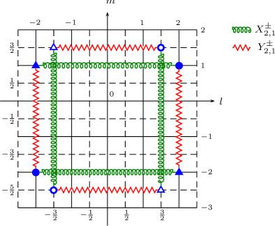
Figure 4: The “intertwining paths”, which correspond to the action of the operators $X_{2,1}^{\pm}$ and $Y_{2,1}^{\pm}$ between the mutually shifted, self-isospectral Hamiltonians (presented by circles and triangles), are shown for the case of the extended $\mathcal{PT}$-symmetric system $\mathcal{H}_{2,1}=\mathcal{H}_{\frac{3}{2},\frac{3}{2}}$. The effect produced by these intertwining operators on the integer-valued lattice is the same as that of the discrete operators ${\cal R}_{l}$ and ${\cal R}_{m}$, respectively. On the half-integer-valued lattice, the horizontal and vertical distances between the corresponding systems are interchanged, and in this sense, the action of the operators $X_{2,1}^{\pm}$ and $Y_{2,1}^{\pm}$ on the half-integer-valued lattice is dual to that on the integer-valued lattice. Starting from any point, the composition of horizontal and vertical paths to the equivalent point on the same lattice produces the Lax integrals $Z_{2,1}^{\pm}$ and the symmetry operator ${\cal R}_{l}{\cal R}_{m}$.

It is straightforward to check from the above relations that ${\cal Z}_{l,m}$ commutes with the Hamiltonian (4.2) and with the integrals ${\cal X}_{l,m}$ and ${\cal Y}_{l,m}$,

$$[{\cal Z}_{l,m},{\cal X}_{l,m}]=0,\qquad[{\cal Z}_{l,m},{\cal Y}_{l,m}]=0\,.$$ (4.32)

Its square produces a polynomial in ${\cal H}_{l,m}$,

$${\cal P}_{{\cal Z}}({\cal H}_{l,m})={\cal H}_{l,m}\prod^{m-1}_{r=0}\prod^{[l-1/2]}_{s=0}({\cal H}_{l,m}+(m-r)^{2})^{2}({\cal H}_{l,m}+(l-s-1/2)^{2})^{2}\,.$$ (4.33)

whose roots are all the discrete doubly degenerate energies of the extended system. Note that the roots of the bound states are of degree two, while the zero energy state root has degree one. All the corresponding energy eigenstates are the zero modes of the integral ${\cal Z}_{l,m}$,

$${\cal Z}_{l,m}\Phi_{n,l}^{\pm}=0,\qquad{\cal Z}_{l,m}\Phi_{n,m}^{\pm}=0,$$ (4.34)

which also detects the direction of propagation of the waves of the scattering sector,

$${\cal Z}_{l,m}\Phi^{\pm}_{+k} = -(-1)^{m+l}k\prod^{m-1}_{r=0}\prod^{[l-1/2]}_{s=0}(k^{2}+(m-r)^{2})(k^{2}+(l-s-1/2)^{2})\Phi^{\pm}_{+k}\,,$$ (4.35)

$${\cal Z}_{l,m}\Phi^{\pm}_{-k} = (-1)^{m+l}k\prod^{m-1}_{r=0}\prod^{[l-1/2]}_{s=0}((k^{2}+(m-r)^{2})k^{2}+(l-s-1/2)^{2})\Phi^{\pm}_{-k}\,.$$ (4.36)

Because of the $\mathcal{PT}$-odd nature of the operators $A^{\pm}_{l,m}$ and $B^{\pm}_{l,m}$, from which ${\cal X}_{l,m}$, ${\cal Y}_{l,m}$ and ${\cal Z}_{l,m}$ are composed, all this triplet of the integrals is $\mathcal{PT}$-even. Thus, instead to be Hermitian operators, all the conserved quantities commute with the ${\cal PT}$ operator,

$$[{\cal H}_{l,m},{\cal PT}]=0,\quad[{\cal X}_{l,m},{\cal PT}]=0,\quad[{\cal Y}_{l,m},{\cal PT}]=0,\quad[{\cal Z}_{l,m},{\cal PT}]=0\,.$$ (4.37)

It is this property of the $\mathcal{PT}$-symmetry that requires the presence of the imaginary unit as a multiplicative factor in the definition of ${\cal Y}_{l,m}$ in Eq. (4.21). In turn, the factor $i$ in Eq. (4.21) emphasizes then the existence of the splitting of the discrete eigenstates into two different families, and reveals an additional specific feature of the whole supersymmetric configuration we have here. The simultaneous requirement of a common basis of eigenstates for all the integrals of motion in addition to the relation (4.37) fixes that only the integral ${\cal Y}_{l,m}$ has imaginary eigenvalues for the set of doublet states $\Phi_{n,l}^{\pm}$ in Eq. (4.4) (see Eq. (4.24) and also the examples in the next section). As all the integrals are mutually commuting operators, the picture here is different from that in a usual quantum mechanics where Hermitian (self-adjoint) mutually commuting operators possess a common basis of eigenstates with real eigenvalues. It is instructive to look in more detail what happens here. Explicit form of the states in (4.4) shows that they are not the eigenstates of the ${\cal PT}$ operator. Indeed, they satisfies the relation

$${\cal PT}\Phi_{n,l}^{\pm}=\Phi_{n,l}^{\mp}\,.$$ (4.38)

Remembering that ${\cal X}_{l,m}$ and ${\cal Z}_{l,m}$ annihilate the set of doublet states (4.4), while the extended Hamiltonian (4.1) has an entire real spectrum [and the states (4.4) are its eigenstates], one concludes that the ${\cal PT}$-symmetry has a broken nature just for the integral ${\cal Y}_{l,m}$ [we remind parenthetically here that the eigenstates from the continuous part of the spectrum have real eigenvalues for ${\cal Y}_{l,m}$, see Eqs. (4.25) and (4.26)]. Taking into account independently only the Hamiltonian operator, one can find another basis where these states are simultaneously the eigenstates of the Hamiltonian and the ${\cal PT}$ operator; therefore, for the ${\cal H}_{l,m}$ the ${\cal PT}$-symmetry is unbroken.

We have identified the nontrivial integrals of the extended system and discussed their properties. Now we consider the related nonlinear supersymmetric structure. The diagonal matrix $\sigma_{3}$ is a trivial integral of motion for $\mathcal{H}_{l,m}$. Nevertheless it allows us to double the set of the nontrivial integrals of motion since the multiplication of any of them by $\sigma_{3}$ gives a new, linear independent nontrivial matrix integral of motion. So, in this way we obtain the set of six linearly independent nontrivial matrix integrals of motion

$$\mathcal{Q}^{(1)}_{l,m}={\cal X}_{l,m}\,,\qquad\mathcal{Q}^{(2)}_{l,m}=\sigma_{3}\mathcal{Q}^{(1)}_{l,m}\,,$$ (4.39)

$$\mathcal{S}^{(1)}_{l,m}={\cal Y}_{l,m}\,,\qquad\mathcal{S}^{(2)}_{l,m}=\sigma_{3}\mathcal{S}^{(1)}_{l,m}\,,$$ (4.40)

$$\mathcal{L}^{(1)}=\mathcal{Z}_{l,m}\,,\qquad\mathcal{L}^{(2)}=\sigma_{3}\mathcal{L}^{(1)}_{l,m}\,.$$ (4.41)

Notice the absence of the imaginary factor $i$ in the definition of the second anti-diagonal supercharges in comparison with the usual SUSYQM approach with a Hermitian Hamiltonian. This guarantees that all the three new integrals are also ${\cal PT}$-symmetric operators.

The square of the matrix integral $\sigma_{3}$ equals $1$, and it can be identified as the grading operator, $\Gamma=\sigma_{3}$. This grading operator classifies then the Hamiltonian $\mathcal{H}_{l,m}$ and integrals $\mathcal{L}^{(a)}_{l,m}$, $a=1,2$, as bosonic operators, while the integrals of the antidiagonal matrix form, $\mathcal{Q}^{(a)}_{l,m}$ and $\mathcal{S}^{(a)}_{l,m}$, are classified as fermionic operators. In correspondence with this, we get a nonlinear superalgebra with the following set of nontrivial (anti)-commutation relations:

$$\{\mathcal{Q}^{(a)}_{l,m},\mathcal{Q}^{(b)}_{l,m}\}=(-1)^{a+1}2\delta_{ab}P_{{\cal X}},\,\,\{\mathcal{S}^{(a)}_{l,m},\mathcal{S}^{(b)}_{l,m}\}=(-1)^{a+1}2\delta_{ab}P_{{\cal Y}},\,\,\{\mathcal{Q}^{(a)}_{l,m},\mathcal{S}^{(b)}_{l,m}\}=-2\delta_{ab}\mathcal{L}^{(1)}_{l,m}\,,$$

$$[\mathcal{Q}^{(a)}_{l,m},\mathcal{L}^{(2)}_{l,m}]=(-1)^{a}2\epsilon_{ab}\mathcal{S}^{(b)}_{l,m}P_{{\cal X}},\quad[\mathcal{S}^{(a)}_{l,m},\mathcal{L}^{(2)}_{l,m}]=(-1)^{a}2\epsilon_{ab}\mathcal{Q}^{(b)}_{l,m}P_{{\cal Y}}\,,$$ (4.42)

where $P_{{\cal X}}=P_{{\cal X}}(\mathcal{H}_{l,m})$ and $P_{{\cal Y}}=P_{{\cal Y}}(\mathcal{H}_{l,m})$ are the polynomials defined in (4.15), (4.23) and (4.33), respectively. Note that the integral $\mathcal{L}^{(1)}_{l,m}$ commutes with all the other integrals and, so, plays here the role of the bosonic central charge.

The choice of $\sigma_{3}$ as the grading operator is, however, not unique. Another possibility corresponds, for instance, to the choice $\Gamma=\mathcal{P}T_{+}$ (or, $\Gamma=\mathcal{P}T_{-}$). Indeed, this operator is a (nonlocal) integral of motion, whose square is equal to $1$. Such a grading operator classifies the integrals $\mathcal{Q}^{(a)}_{l,m}$ as bosonic integrals, while $\mathcal{S}^{(a)}_{l,m}$ and $\mathcal{L}^{(a)}_{l,m}$ are classified as fermionic integrals. The corresponding superalgebraic relations can be computed then by making use of the relations described above. In this case we have, particularly, a relation $\{\mathcal{L}^{(a)}_{l,m},\mathcal{L}^{(b)}_{l,m}\}=2\delta_{ab}P_{{\cal Z}}(\mathcal{H}_{l,m})$. This corresponds to the fact that each of the unextended $\mathcal{PT}$-symmetric systems $H^{+}_{l,m}$ and $H^{-}_{l,m}$ is characterized by the bosonized supersymmetry, in which the $\mathcal{PT}$-symmetric integrals $iZ^{+}_{l,m}$ and $iZ^{-}_{l,m}$, respectively, are treated as the $\Gamma=\mathcal{P}T_{+}$-odd supercharges.

We summarize the whole picture on which the tri-supersymmetric structure is based on Fig. 5.

Figure 5: The basic blocks of the tri-supersymmetric structure of the extended $\mathcal{PT}$-symmetric Hamiltonian $\mathcal{H}_{l,m}$. Horizontal arrows inside a table correspond to the duality transformation induced by the symmetry $(l,m)\rightarrow\left(m+\frac{1}{2},l-\frac{1}{2}\right)$.

5 Examples

To illustrate different properties of the systems $H^{\pm}_{l,m}$ and the tri-supersymmetric structure of $\mathcal{H}_{l,m}$, here we present some examples for specific values of $l$ and $m$. Before doing this, we first note that according to the relation (2.14), the simplest nontrivial case of $H^{+}_{1,0}(x)=H^{-}_{1,0}(x+i\pi)$ reduces, up to rescaling, just to the displaced reflectionless Pöschl-Teller system with one bound state in the spectrum. The unique bound state corresponds to a resonance with a complex energy value in the spectrum of the Hermitian Hamiltonian with real Scarf II potential $V(x)={\rm sech}^{2}(x)-\sinh x\,{\rm sech}^{2}x$, which is depicted on Fig. 2. So we will consider more rich cases of reflectionless $\mathcal{PT}$-symmetric systems with two and three bound states.

5.1 Systems with two bound states

Without loss of generality, the family of reflectionless potentials $V^{\pm}_{l,m}$ with two bound states in the discrete part of the spectrum can be presented by non-negative integer values of the parameters $l$ and $m$ subjected to the condition $l+m=2$. The case $(l=0,m=2)$ corresponds here to the well known Hermitian reflectionless Pöschl-Teller potential $V_{0,2}^{+}=V_{0,2}^{-}=-6/\cosh^{2}x$. By virtue of (2.14), this potential shares, up to rescaling, the same spectrum as complexified Scarf II potentials with $(l=1,m=1)$. Then the remaining case $(l=2,m=0)$,

$$H^{\pm}_{2,0}=-\frac{d^{2}}{dx^{2}}-\frac{4}{\cosh^{2}x}\pm 2i\frac{\sinh x}{\cosh^{2}x}\,,$$ (5.1)

provides a first nontrivial example which is not related to a Hermitian (reflectionless Pöschl-Teller) counterpart by means of shifting and rescaling of the coordinate. The potentials $V=V_{2,0}^{\pm}$ are solutions of the nonlinear $s$-KdV₂ equation

$$V^{(5)}-10V^{\prime\prime\prime}V-20V^{\prime}V^{\prime\prime}+30V^{2}V^{\prime}-10(V^{\prime\prime\prime}-3VV^{\prime})+9V^{\prime}=0\,,$$ (5.2)

where $V^{(5)}=d\,^{5}V/dx^{5}$. Notice that in contrast with the complexified case $V_{2,0}^{\pm}$, the Hermitian version of the potential, $V_{2i,0}$, which is plotted on Fig. 2, is not a solution of the $s$-KdV₂ equation. The Hamiltonians $H^{\pm}_{2,0}$ fall into the class of systems studied in [38] in the context of the $\mathcal{PT}-$symmetric nonlinear integrable systems; the corresponding extended Hamiltonian $\mathcal{H}_{2,0}$ appears as a particular case of the diagonalized squared Dirac equation for a free spin-1/2 field in de Sitter space, see Ref. [37].

The degeneracy of the spectrum of ${\cal H}_{2,0}$ is twice that for each system in (5.1), and we have two doublets of bound states and two zero energy states at the very bottom of the four-fold degenerate continuous part of the spectrum. The bound states correspond here to the complex energy resonances in the Hermitian version with real Scarf II potential, see Fig. 2. Their eigenfunctions,

$$\Phi_{0,l}^{\pm}=\left(\begin{array}[]{c}\displaystyle\frac{e^{-\frac{i}{2}\arctan\sinh x}}{\cosh^{3/2}x}\\ \\ \displaystyle\pm i\frac{e^{\frac{i}{2}\arctan\sinh x}}{\cosh^{3/2}x}\end{array}\right),\quad\Phi_{1,l}^{\pm}=\left(\begin{array}[]{c}\displaystyle\frac{e^{-\frac{i}{2}\arctan\sinh x}}{\cosh^{3/2}x}(1-2i\sinh x)\\ \\ \displaystyle\pm i\frac{e^{\frac{i}{2}\arctan\sinh x}}{\cosh^{3/2}x}(1+2i\sinh x)\end{array}\right),$$ (5.3)

satisfy equations

$${\cal H}_{2,0}\Phi_{0,l}^{\pm}=-\frac{9}{4}\Phi_{0,l}^{\pm},\qquad{\cal H}_{2,0}\Phi_{1,l}^{\pm}=-\frac{1}{4}\Phi_{1,l}^{\pm}\,,$$ (5.4)

and correspond to wavefunctions (4.4).

These solutions can be obtained from the non-physical states of the free particle, by applicacion of the operators (3.11) or (3.12) with $l=2$ and $m=0$ in the case of the subsystem $H^{+}_{2,0}$. For generic values of $l$ and $m$, the Darboux-Crum transformations that map the free particle eigenstates into those for the lower Hamiltonian $H^{-}_{l,m}$ are realized in correspondence with intertwining relations (5.5) by means of the operators

$${\cal D}_{l,m}^{\sharp} = {\cal P}({\cal D}_{l,m}^{-}){\cal P}={\cal T}({\cal D}_{l,m}^{-}){\cal T}\,,$$ (5.5)

$$\tilde{{\cal D}}_{l,m}^{\sharp} = -{\cal P}(\tilde{{\cal D}}_{l,m}^{-}){\cal P}=-{\cal T}(\tilde{{\cal D}}_{l,m}^{-}){\cal T}\,.$$ (5.6)

Note that in correspondence with relation $H^{-}_{l,m}(x)=H^{+}_{l,m}(x+i\pi)$, operators (5.5) are obtained equivalently from the intertwining operators ${\cal D}_{l,m}^{-}$ and $\tilde{{\cal D}}_{l,m}^{-}$ by the half-period shift. The non-physical states which are transformed into bound states by means of the Darboux-Crum transformations (3.11), (3.12), (5.5) and (5.6) are

$$\phi_{-9/4}^{+}=\cosh\left(\frac{3x}{2}\right),\qquad\phi_{-9/4}^{-}=\sinh\left(\frac{3x}{2}\right)\,,$$ (5.7)

and

$$\phi_{-1/4}^{+}=\cosh\left(\frac{x}{2}\right),\qquad\phi_{-1/4}^{-}=\sinh\left(\frac{x}{2}\right)\,,$$ (5.8)

which obey the same Schrödinger equations as in (5.4),

$$H_{0}\,\phi_{-9/4}^{\pm}=-\frac{9}{4}\phi_{-9/4}^{\pm},\quad H_{0}\,\phi_{-1/4}^{\pm}=-\frac{1}{4}\phi_{-1/4}^{\pm}\,.$$ (5.9)

One can choose solutions of different parity with respect to ${\cal P}$ in (5.7) and (5.8) to obtain the bound states (5.3). Choosing the functions with positive ${\cal P}$-parity we have,

$$\Phi_{0,l}^{\pm} = \frac{2}{3}\left(\begin{array}[]{c}{\cal D}_{2,0}^{-}\\ \pm i\,{\cal D}_{2,0}^{\sharp}\end{array}\right)\phi_{-9/4}^{+}=\frac{4i}{9}\left(\begin{array}[]{c}\tilde{{\cal D}}_{2,0}^{-}\\ \mp i\,\tilde{{\cal D}}_{2,0}^{\sharp}\end{array}\right)\phi_{-9/4}^{+}\,,$$ (5.14)

$$\Phi_{1,l}^{\pm} = -2\left(\begin{array}[]{c}{\cal D}_{2,0}^{-}\\ \pm i\,{\cal D}_{2,0}^{\sharp}\end{array}\right)\phi_{-1/4}^{+}=4i\left(\begin{array}[]{c}\tilde{{\cal D}}_{2,0}^{-}\\ \mp i\,\tilde{{\cal D}}_{2,0}^{\sharp}\end{array}\right)\phi_{-1/4}^{+}\,,$$ (5.19)

where ${\cal D}_{2,0}^{-}=A^{-}_{2,0}A^{-}_{1,0}$, $\tilde{{\cal D}}_{2,0}^{-}=B^{+}_{-2,0}A^{+}_{-1,0}A^{+}_{0,0}$, ${\cal D}_{2,0}^{\sharp}=A^{-}_{0,-1}A^{-}_{-1,1}$, $\tilde{{\cal D}}_{2,0}^{\sharp}=B^{+}_{2,0}A^{-}_{2,0}A^{-}_{1,0}$. Expressions (5.14) and (5.19) with the non-physical states of ${\cal P}$-negative parity, i.e. $\phi_{-9/4}^{-}$ and $\phi_{-1/4}^{-}$, remain almost identical up to multiplicative constant factors. One can choose these factors pure imaginary to produce, for each entry of (5.14) and (5.19), a state of definite ${\cal PT}$-parity by starting from $\phi_{-9/4}^{\pm}$ or $\phi_{-1/4}^{\pm}$. This can be understood by taking into account that the intertwining operators have no definite ${\cal P}$-parity, but they have a definite ${\cal PT}$-parity. In general case, while the ${\cal D}_{l,m}^{-}$ and ${\cal D}_{l,m}^{\sharp}$ are ${\cal PT}$-even, the operators $\tilde{{\cal D}}_{l,m}^{-}$ and $\tilde{{\cal D}}_{l,m}^{\sharp}$ are ${\cal PT}$-odd.

Using the same procedure as with bound states, we can construct the eigenstates in the scattering sector (4.6) by applying the intertwining Darboux-Crum operators to the plane waves (3.15) of $H_{0}$,

$$\Phi_{+k}^{\pm}=\left(\begin{array}[]{c}{\cal D}_{2,0}^{-}\\ \pm\,{\cal D}_{2,0}^{\sharp}\end{array}\right)e^{ikx},\qquad\Phi_{-k}^{\pm}=\left(\begin{array}[]{c}{\cal D}_{2,0}^{-}\\ \pm\,{\cal D}_{2,0}^{\sharp}\end{array}\right)e^{-ikx}\,,$$ (5.20)

$${\cal H}_{2,0}\Phi_{+k}^{\pm}=k^{2}\Phi_{+k}^{\pm}\,,\qquad{\cal H}_{2,0}\Phi_{-k}^{\pm}=k^{2}\Phi_{-k}^{\pm}\,.$$ (5.21)

The eigenfunctions (5.20) for $H_{2,0}^{+}$ and $H_{2,0}^{-}$ may also be obtained by applying, instead, the operators $\tilde{{\cal D}}_{2,0}^{-}$ and $\tilde{{\cal D}}_{2,0}^{\sharp}$, respectively, to the same plane wave eigenstates. In the case of the zero energy eigenstates we have

$$\Phi_{0}^{\pm}=\left(\begin{array}[]{c}{\cal D}_{2,0}^{-}\\ \pm\,{\cal D}_{2,0}^{\sharp}\end{array}\right)1=\left(\begin{array}[]{c}\tilde{{\cal D}}_{2,0}^{-}\\ \pm\,\tilde{{\cal D}}_{2,0}^{\sharp}\end{array}\right)x=-\frac{3}{4}\left(\begin{array}[]{c}e^{-2i\arctan\sinh x}\\ \pm e^{2i\arctan\sinh x}\end{array}\right),$$ (5.22)

i. e. the operators $\tilde{{\cal D}}_{2,0}^{-}$ and $\tilde{{\cal D}}_{2,0}^{\sharp}$ should act on the non-physical zero energy solutions of $H_{0}$ which are proportional to $x$. Another solution of zero energy of $H_{0}$, which is a constant, is annihilated by the Darboux-Crum operators,

$$\tilde{{\cal D}}_{2,0}^{-}1=\tilde{{\cal D}}_{2,0}^{\sharp}1=0\,.$$ (5.23)

The extended Hamiltonian ${\cal H}_{2,0}$ possesses three basic conserved quantities in the form of the matrix differential operators. One of these integrals, ${\cal X}_{2,0}$, is given by

$${\cal X}_{2,0}=\left(\begin{array}[]{cc}0&X_{2,0}^{-}\\ X_{2,0}^{+}&0\end{array}\right)=\left(\begin{array}[]{cc}0&A_{2,0}^{-}A_{1,0}^{-}A_{0,0}^{-}A_{-1,0}^{-}\\ A_{-1,0}^{+}A_{0,0}^{+}A_{1,0}^{+}A_{2,0}^{+}&0\end{array}\right)\,.$$ (5.24)

The explicit form of the higher order differential operators is

$$X^{\pm}_{2,0}=\frac{d^{4}}{dx^{4}}\pm\frac{2i}{\cosh x}\frac{d^{3}}{dx^{3}}+\frac{1}{\cosh^{2}x}\left(6\mp 3i\sinh x-\frac{5}{2}\cosh^{2}x\right)\frac{d^{2}}{dx^{2}}$$ (5.25)

$$-\frac{1}{\cosh^{3}x}\left(12\sinh x\pm i\left[\frac{1}{2}\cosh^{2}x-3\right]\right)\frac{d}{dx}-\frac{13}{\cosh^{4}x}\left(13\mp 3i\sinh x\right)\left(1\pm i\sinh x\right)^{3}\,.$$

This integral acts on the physical states of the Hamiltonian ${\cal H}_{2,0}$ as follows,

$${\cal X}_{2,0}\Phi_{0,l}^{\pm}=0,\quad{\cal X}_{2,0}\Phi_{1,l}^{\pm}=0,\quad{\cal X}_{2,0}\Phi_{0}^{\pm}=\pm\frac{9}{16}\Phi_{0}^{\pm},\quad$$ (5.26)

$${\cal X}_{2,0}\Phi_{+k}^{\pm}=\pm\left(k^{2}+\frac{1}{4}\right)\left(k^{2}+\frac{9}{4}\right)\Phi_{+k}^{\pm},\quad{\cal X}_{2,0}\Phi_{-k}^{\pm}=\pm\left(k^{2}+\frac{1}{4}\right)\left(k^{2}+\frac{9}{4}\right)\Phi_{-k}^{\pm}\,.$$ (5.27)

The operator ${\cal X}_{2,0}$ does not distinguish the waves coming from the left or the right, but recognizes the states which correspond to resonances in the Hermitian Scarf II potential spectrum, by annihilating all of them. Another integral of motion is also an anti-diagonal matrix differential operator,

$${\cal Y}_{2,0}=i\left(\begin{array}[]{cc}0&Y_{2,0}^{-}\\ Y_{2,0}^{+}&0\end{array}\right)=i\left(\begin{array}[]{cc}0&B_{2,0}^{-}\\ B_{2,0}^{+}&0\end{array}\right)\,,$$ (5.28)

where

$$Y_{2,0}^{\pm}=B_{2,0}^{\pm}=\frac{d}{dx}\pm i\frac{2}{\cosh x}\,.$$ (5.29)

The integral of motion ${\cal Y}_{2,0}$ commutes with ${\cal X}_{2,0}$ and encodes the information to be complementary to that provided by the latter. This can be seen from its action on the physical states,

$${\cal Y}_{2,0}\Phi_{0,l}^{\pm}=\pm\frac{3i}{2}\Phi_{0,l}^{\pm},\qquad{\cal Y}_{2,0}\Phi_{1,l}^{\pm}=\pm\frac{i}{2}\Phi_{1,l}^{\pm},\qquad{\cal Y}_{2,0}\Phi_{k}^{\pm}=0,\quad$$ (5.30)

$${\cal Y}_{2,0}\Phi_{+k}^{\pm}=\mp k\Phi_{+k}^{\pm},\qquad{\cal Y}_{2,0}\Phi_{-k}^{\pm}=\pm k\Phi_{-k}^{\pm}\,.$$ (5.31)

The remaining doublet states are annihilated by ${\cal Y}_{2,0}$, which in this case correspond to the states of the zero energy at the bottom of the continuous spectrum. The waves coming from the left or the right are recognized by it, and like (5.24), the ${\cal Y}_{2,0}$ detects also the upper index of eigenstates. Note that the bound eigenstates here that correspond to resonances in the Hermitian Scarf II systems spectra have pure imaginary eigenvalues of ${\cal Y}_{2,0}$.

Coherently with the properties of the displayed antidiagonal integrals, the diagonal operator ${\cal Z}_{2,0}=\mathcal{X}_{2,0}\mathcal{Y}_{2,0}$ annihilates all the doublet states, and separates scattering states coming from different directions,

$${\cal Z}_{2,0}\Phi_{0,l}^{\pm}=0,\qquad{\cal Z}_{2,0}\Phi_{1,l}^{\pm}=0,\qquad{\cal Z}_{2,0}\Phi_{0}^{\pm}=0\,,$$ (5.32)

$${\cal Z}_{2,0}\Phi_{+k}^{\pm}=-k\left(k^{2}+\frac{1}{4}\right)\left(k^{2}+\frac{9}{4}\right)\Phi_{+k}^{\pm},\quad{\cal Z}_{2,0}\Phi_{-k}^{\pm}=k\left(k^{2}+\frac{1}{4}\right)\left(k^{2}+\frac{9}{4}\right)\Phi_{-k}^{\pm}\,.$$ (5.33)

5.1.1 Systems with three bound states

Reflectionless systems with three bound states are constrained to fullfill the relation $l+m=3$. Potentials (2.1) with $(l=0,m=3)$ and $(l=2,m=1)$ are related by Eq. (2.14). When $(l=3,m=0)$, the systems $H^{\pm}_{3,0}$ have three bound states, all of which correspond to resonance states in the Hermitian version. So, all the mentioned three bound states systems have corresponding analogs in more simple cases we have discussed above. A more non-trivial example with three bound states is given by the Hamiltonians

$$H^{\pm}_{1,2}=-\frac{d^{2}}{dx^{2}}-\frac{7}{\cosh^{2}x}\pm 5i\frac{\sinh x}{\cosh^{2}x}\,.$$ (5.34)

The Hermitian counterpart potential for $H^{+}_{1,2}$ is shown on Fig. 2. Here the potentials $V=V^{\pm}_{1,2}$ satisfy the $s$-KdV₃ equation

$$V^{(7)}-14V(V^{(5)}-20V^{\prime\prime}V^{\prime})-42V^{(4)}V^{\prime}-70V^{\prime\prime\prime}V^{\prime\prime}+70V^{\prime\prime\prime}V^{2}+70V^{\prime 3}-140V^{\prime}V^{3}+$$

$$-21(V^{(5)}-10V^{\prime\prime\prime}V-20V^{\prime}V^{\prime\prime}+30V^{2}V^{\prime})+84(V^{\prime\prime\prime}-6VV^{\prime})-64V^{\prime}=0\,.$$ (5.35)

The extended Hamiltonian ${\cal H}_{1,2}$ has six bound states, where four correspond to the bound state from the set (3.1),

$$\Phi_{0,m}^{\pm}=\left(\begin{array}[]{c}\displaystyle\frac{e^{-i\arctan\sinh x}}{\cosh^{2}x}\\ \\ \pm\displaystyle\frac{e^{i\arctan\sinh x}}{\cosh^{2}x}\end{array}\right),\quad\Phi_{1,m}^{\pm}=\left(\begin{array}[]{c}\displaystyle\frac{e^{\mp i\arctan\sinh x}}{\cosh^{2}x}(2-3i\sinh x)\\ \\ \displaystyle\pm\frac{e^{\mp i\arctan\sinh x}}{\cosh^{2}x}(2+3i\sinh x)\end{array}\right),$$ (5.36)

$${\cal H}_{1,2}\Phi_{0,m}^{\pm}=-4\Phi_{0,m}^{\pm},\qquad{\cal H}_{1,2}\Phi_{1,m}^{\pm}=-\Phi_{1,m}^{\pm}\,.$$ (5.37)

These solutions are analogs of the bound states for the Hermitian counterpart system, which, in addition, admits resonances for a complex value of energy. Those resonances correspond to two extra bound states solutions in the spectrum of the Hamiltonian ${\cal H}_{1,2}$,

$$\Phi_{0,l}^{\pm}=\left(\begin{array}[]{c}\displaystyle\frac{e^{-\frac{5i}{2}\arctan\sinh x}}{\cosh^{1/2}x}\\ \\ \displaystyle\pm i\frac{e^{\frac{5i}{2}\arctan\sinh x}}{\cosh^{1/2}x}\end{array}\right)\,,\qquad{\cal H}_{1,2}\Phi_{0,l}^{\pm}=-\frac{1}{4}\Phi_{0,l}^{\pm}\,.$$ (5.38)

All the bound states described above, $\Phi_{0,m}$, $\Phi_{1,m}$ and $\Phi_{0,l}$, can be derived from the non-physical states of the free particle, $\phi_{-4}^{\pm}$, $\phi_{-1}^{\pm}$ and $\phi_{-1/4}^{\pm}$, respectively. Here, the unphysical solutions of $H_{0}$ are

$$\phi_{-4}^{+}=\cosh 2x,\qquad\phi_{-4}^{-}=\sinh 2x\,,$$ (5.39)

and

$$\phi_{-1}^{+}=\cosh x,\qquad\phi_{-1}^{-}=\sinh x\,;$$ (5.40)

they have the same eigenvalues (of $H_{0}$) as the bound states $\Phi_{0,m}^{\pm}$ and $\Phi_{1,ml}^{\pm}$ in (5.37). The mapping between the states is given by

$$\Phi_{0,m}^{\pm}=\frac{2i}{15}\left(\begin{array}[]{c}{\cal D}_{1,2}^{-}\\ \mp\,{\cal D}_{1,2}^{\sharp}\end{array}\right)\phi_{-4}^{+},\quad\Phi_{1,m}^{\pm}=-\frac{2}{3}\left(\begin{array}[]{c}{\cal D}_{1,2}^{-}\\ \pm\,{\cal D}_{1,2}^{\sharp}\end{array}\right)\phi_{-1}^{+},\quad\Phi_{0,l}^{\pm}=-\frac{8}{15}\left(\begin{array}[]{c}{\cal D}_{1,2}^{-}\\ \pm i\,{\cal D}_{1,2}^{\sharp}\end{array}\right)\phi_{-1/4}^{-}\,,$$ (5.47)

where we use the definition of the operators (3.11) and (5.5). Similar expressions can be found by making use of the operators (3.12) and (5.6); it is worth to note, however, that some non-physical states of the free particle cannot be mapped properly because are annihilated,

$${\cal D}_{1,2}^{-}\phi_{-4}^{-}={\cal D}_{1,2}^{\sharp}\phi_{-4}^{-}={\tilde{\cal D}}_{1,2}^{-}\phi_{-4}^{+}={\tilde{\cal D}}_{1,2}^{\sharp}\phi_{-4}^{+}=0\,,$$ (5.48)

$${\cal D}_{1,2}^{+}\phi_{-1}^{-}={\cal D}_{1,2}^{\sharp}\phi_{-1}^{+}={\tilde{\cal D}}_{1,2}^{-}\phi_{-1}^{-}={\tilde{\cal D}}_{1,2}^{\sharp}\phi_{-1}^{-}=0\,.$$ (5.49)

The situation is quite similar to the previous case (5.23). In fact, in this case the constant state of the free particle is also annihilated by the operators ${\tilde{\cal D}}_{1,2}^{-}1={\tilde{\cal D}}_{1,2}^{\sharp}1=0$.

The wave functions of the continuum are obtained by the same method from the free plane waves,

$$\Phi_{+k}^{\pm}=\left(\begin{array}[]{c}{\cal D}_{1,2}^{-}\\ \pm{\cal D}_{1,2}^{\sharp}\end{array}\right)e^{ikx},\qquad\Phi_{-k}^{\pm}=\left(\begin{array}[]{c}{\cal D}_{1,2}^{-}\\ \pm{\cal D}_{1,2}^{\sharp}\end{array}\right)e^{-ikx}\,,$$ (5.50)

and have energies $E=k^{2}$.

The anti-diagonal, mutually commuting basic integrals of motion for this case, ${\cal X}_{1,2}$ and ${\cal Y}_{1,2}$, have differential orders $|{\cal X}_{1,2}|=2$ and $|{\cal Y}_{1,2}|=5$, and read

$${\cal X}_{1,2}=\left(\begin{array}[]{cc}0&X_{1,2}^{-}\\ X_{1,2}^{+}&0\end{array}\right)=\left(\begin{array}[]{cc}0&A_{1,2}^{-}A_{2,0}^{-}\\ A_{2,0}^{+}A_{1,2}^{+}&0\end{array}\right)\,,$$ (5.51)

and

$${\cal Y}_{1,2}=i\left(\begin{array}[]{cc}0&Y_{1,2}^{-}\\ Y_{1,2}^{+}&0\end{array}\right)=i\left(\begin{array}[]{cc}0&B_{1,2}^{-}B_{1,1}^{-}B_{1,0}^{-}B_{1,-1}^{-}B_{1,-2}^{-}\\ B_{1,-2}^{+}B_{1,-1}^{+}B_{1,0}^{+}B_{1,1}^{+}B_{1,2}^{+}&0\end{array}\right)\,.$$ (5.52)

The explicit form of differential operators that compose (5.51) and (5.52) are

$$X_{1,2}^{\pm}=\frac{d^{2}}{dx^{2}}\pm\frac{5i}{\cosh x}\frac{d}{dx}-\frac{1}{8\cosh^{2}x}\left(44+\cosh^{2}x\pm 20i\sinh x\right)$$ (5.53)

and

$$Y_{1,2}^{\pm}=\frac{d^{5}}{dx^{5}}\pm\frac{5i}{\cosh x}\frac{d^{4}}{dx^{4}}-\frac{5}{\cosh^{2}x}\left(\sinh^{2}x\pm 2i\sinh x\right)\frac{d^{3}}{dx^{3}}-\frac{5}{\cosh^{3}x}\left(3\sinh x\mp 2i\pm i\sinh^{2}x\right)\frac{d^{2}}{dx^{2}}$$

$$+\frac{1}{\cosh^{4}x}\left(4\cosh^{4}x+10\cosh^{2}x-30\mp 65i\sinh x\pm 10i\sinh x\right)\frac{d}{dx}$$

$$-\frac{15}{\cosh^{5}x}\left(2\sinh x\mp 5i\pm 4i\cosh^{2}x\right)\,.$$

The action of the integrals on the doublets of the Hamiltonian is given by

$${\cal X}_{1,2}\Phi_{0,m}^{\pm}=\mp\frac{15}{4}\Phi_{0,m}^{\pm},\quad{\cal X}_{1,2}\Phi_{1,m}^{\pm}=\pm\frac{3}{4}\Phi_{1,m}^{\pm},\quad{\cal X}_{1,2}\Phi_{0,l}^{\pm}=0,\quad{\cal X}_{1,2}\Phi_{0,l}^{\pm}=\pm\frac{1}{4}\Psi_{k,0}^{\pm},$$ (5.54)

$${\cal Y}_{1,2}\Phi_{0,m}^{\pm}=0,\quad{\cal Y}_{1,2}\Phi_{1,m}^{\pm}=0,\quad{\cal Y}_{1,2}\Phi_{0,l}^{\pm}=\pm\frac{45i}{32}\Phi_{0,l}^{\pm},\quad{\cal Y}_{1,2}\Phi_{0}^{\pm}=0\,.$$ (5.55)

Note that, again, the states $\Phi_{0,l}^{\pm}$, which correspond to resonances in the Hermitian counterpart systems, are annihilated by the integral $\mathcal{X}_{1,2}$ and are characterized by pure imaginary eigenvalues of the second integral $\mathcal{Y}_{1,2}$. The scattering states (5.50) are eigenstates of the operators ${\cal X}_{1,2}$ and ${\cal Y}_{1,2}$,

$${\cal X}_{1,2}\Phi_{+k}^{\pm}=\mp\left(k^{2}+\frac{1}{4}\right)\Phi_{+k}^{\pm},\qquad{\cal X}_{1,2}\Phi_{-k}^{\pm}=\mp\left(k^{2}+\frac{1}{4}\right)\Phi_{-k}^{\pm}\,,$$ (5.56)

$${\cal Y}_{1,2}\Phi_{+k}^{\pm}=\mp k(k^{2}+1)(k^{2}+4)\Phi_{+k}^{\pm},\qquad{\cal Y}_{1,2}\Phi_{-k}^{\pm}=\pm k(k^{2}+1)(k^{2}+4)\Phi_{-k}^{\pm}\,.$$ (5.57)

Finally, the diagonal integral ${\cal Z}_{1,2}={\cal Y}_{1,2}{\cal X}_{1,2}={\cal X}_{1,2}{\cal Y}_{1,2}$ annihilates the whole set of doublet states,

$${\cal Z}_{1,2}\Phi_{0,m}^{\pm}=0,\quad{\cal Z}_{1,2}\Phi_{1,m}^{\pm}=0,\quad{\cal Z}_{1,2}\Phi_{0,l}^{\pm}=0,\quad{\cal Z}_{1,2}\Phi_{0}^{\pm}=0\,,$$ (5.58)

and recognizes, as the integral ${\cal Y}_{1,2}$, the waves coming from the left or the right,

$${\cal Z}_{1,2}\Phi_{+k}^{\pm}=k\left(k^{2}+\frac{1}{4}\right)(k^{2}+1)(k^{2}+4)\Phi_{+k}^{\pm},\quad{\cal Z}_{1,2}\Phi_{-k}^{\pm}=-k\left(k^{2}+\frac{1}{4}\right)(k^{2}+1)(k^{2}+4)\Phi_{-k}^{\pm}\,.$$ (5.59)

6 Discussion and outlook

In this paper, by analyzing a two-parametric family of reflectionless ${\cal PT}$-symmetric Hamiltonians, we have revealed a new supersymmetric structure. The class of potentials studied here provides an instructive example of quantum mechanical systems with non-Hermitian Hamiltonians. In comparison with the Hermitian version of the Scarf II potential, the spectrum of its complexified counterpart contains two series of singlet states discovered earlier within a framework of the group theoretical approach. Surprisingly, this characteristic is imprinted in a tri-supersymmetric structure that is based here on the specific properties of the family of potentials: their pure imaginary period and discrete symmetries of a reflection type in the indexes. Usually, the imaginary period in both Hermitian and non-Hermitian Hamiltonians does not play explicitly an important role at the level of the spectrum, or in supersymmetric aspects. Following the original idea of Dunne and Feinberg for the case of a usual SUSYQM with a linear Lie superalgebraic structure and mutually shifted (on a real line) Hermitian Hamiltonians [16], we construct an extended $\mathcal{PT}$-symmetric system composed by two Hamiltonians with self-isospectral potentials, but now displaced mutually in the half of the imaginary period. The obtained composed system has three basic non-trivial integrals of motion, which in the generic case are the higher order differential operators. The importance of the splitting of the discrete states becomes clear by analyzing these integrals. Two of the anti-diagonal, supercharge-type integrals, ${\cal X}_{l,m}$ and ${\cal Y}_{l,m}$, annihilate separately the two different sets of doublets of the extended system. These mutually commuting integrals generate a third, diagonal integral, ${\cal Z}_{l,m}$, that implies the reflectionless property of the Hamiltonian: it appears as the Lax integral, which together with the Hamiltonian forms the Lax pair. The ${\cal PT}$-operator emerges naturally as a valuable symmetry for the integrals of motion in view of the fact that all of them appear as ${\cal PT}$-symmetric operators, in the same way as the Hamiltonian. Nevertheless, the odd order integral ${\cal Y}_{l,m}$ reveals a finite number of pairs of complex conjugate eigenvalues when acts on the bound states which correspond to resonances with complex conjugate energy values in the Hermitian potential counterpart. We can say therefore that for this integral the ${\cal PT}$-symmetry is spontaneously broken.

The ${\cal PT}$-symmetry is composed of the space inversion, $\mathcal{P}$, and the time reversal, $\mathcal{T}$, operators, which play a role of the intertwiners between the mutually displaced components $H^{+}_{l,m}(x)$ and $H^{-}_{l,m}(x)=H^{+}_{l,m}(x+i\pi)$ of the extended Hamiltonian. In addition to them and the half-period displacement operators, there are other discrete intertwiners, the products of which produce discrete symmetries of the extended system. The commuting operators $\mathcal{R}_{l}:\,(l,m)\rightarrow(-l,m)$ and $\mathcal{R}_{m}:(l,m)\rightarrow(l,-m-1)$ produce, particularly, the same effect as the differential intertwiners $X^{\pm}_{l,m}$ and $Y^{\pm}_{l,m}$, from which the supercharges ${\cal X}_{l,m}$ and ${\cal Y}_{l,m}$ are composed. In addition to a usual choice for the $\mathbb{Z}_{2}$-grading operator $\Gamma=\sigma_{3}$, other choices are also possible. The product of the $\mathcal{P}$ and of the operator of the displacement for the half of the imaginary period is one of them, which also happens to be the grading operator for the hidden, nonlinear bosonized supersymmetries of the subsystems $H^{+}_{l,m}$ and $H^{-}_{l,m}$, where the Lax operators $Z^{+}_{l,m}$ and $Z^{-}_{l,m}$ are identified as the odd supercharges.

On the other hand, the mentioned two sets of the discrete eigenstates can be related between themselves by means of another discrete symmetry of the Hamiltonian, which interchanges the integer-valued lattice of the parameters $l$ and $m$ with the half-integer-valued lattice. It is only for such, integer or half-integer, values of the parameters the complexified Scarf II potentials are reflectionless. The indicated symmetry operation intertwines the operators $A^{\pm}_{l,m}$ and $B^{\pm}_{l,m}$, which are the building blocks for the intertwiners $X^{\pm}_{l,m}$ and $Y^{\pm}_{l,m}$, respectively. As a consequence, the role of the integrals ${\cal X}_{l,m}$ and ${\cal Y}_{l,m}$ is dually interchanged by those specific discrete symmetries. In contrast with the rest of the discrete symmetries, these duality generators have no analog in a form of differential operators.

The supersymmetric structure presented here displays several similarities with the tri-supersymmetric structure in self-isospectral Hermitian finite-gap systems with elliptic potentials studied in [20]. In that class of Hermitian systems, two distinct finite-dimensional representations of $sl(2,\mathbb{R})$ are realized on periodic and antiperiodic band-edge states; like here three basic integrals of motion are present in the extended system, and different choices for the grading operators are also possible. The main difference with the present structure is that the corresponding finite-gap elliptic systems are doubly periodic, in addition to the imaginary period the corresponding systems have also a real period, and there the self-isospectral systems are shifted for the half of their real period. The corresponding tri-supersymmetric systems studied in [20] are described by the associated Lamé potentials, which constitute a subclass of the Darboux-Treibich-Verdier family (2). It is interesting therefore to investigate the question of existence of tri-supersymmetric structure for such a class of doubly periodic ${\cal PT}$-symmetric potentials, where the extended Hamiltonian would unify the self-isospectral partners with a mutual complex displacement.

In the definition of a physically consistent, positively definite inner product for the systems with non-Hermitian Hamiltonians, the existence of the operator ${\cal C}$ of the nature of a charge conjugation operator seems to be crucial [5]. An open question is the existence of such a kind of the operator for the complexified Scarf II potential. One can wonder then if the supersymmetric structure discussed here can be helpful in this sense, specifically, if the ${\cal C}$ can be expressed in terms of, or related to the non-trivial integrals of motion.

Particular cases of the potential with $l\in\mathbb{Z}$ and $m=0$ (and equivalent cases obtained by symmetry transformations of indexes) discussed here appear in quantum field theory in curved space-times [37]. A natural question is if a general case of the complex reflectionless potential plays any role in some related problems, and if the the revealed supersymmetric structure could give some insight to these theories.

Acknowledgements. The work has been partially supported by FONDECYT Grants 1095027 (MP) and 3100123 (FC). FC acknowledges also financial support via the CONICYT grants 79112034 and Anillo ACT-91: “Southern Theoretical Physics Laboratory” (STPLab). MP and FC are grateful, respectively, to CECs and Universidad de Santiago de Chile for hospitality. The Centro de Estudios Científicos (CECs) is funded by the Chilean Government through the Centers of Excellence Base Financing Program of Conicyt.

References

• [1] C. M. Bender, S. Boettcher, “Real spectra in non-Hermitian Hamiltonians having PT symmetry,” Phys. Rev. Lett.  80, 5243 (1998), [arXiv:physics/9712001].
• [2] C. M. Bender, S. Boettcher and P. Meisinger, “PT symmetric quantum mechanics,” J. Math. Phys.  40, 2201 (1999), [arXiv:quant-ph/9809072].
• [3] P. Dorey, C. Dunning and R. Tateo, “Spectral equivalences, Bethe Ansatz equations, and reality properties in PT-symmetric quantum mechanics,” J. Phys.  A 34, 5679 (2001), [arXiv:hep-th/0103051].
• [4] A. Mostafazadeh, “Pseudo-Hermiticity versus PT symmetry. The necessary condition for the reality of the spectrum,” J. Math. Phys.  43, 205 (2002), [arXiv:math-ph/0107001]; “Pseudo-Hermiticity versus PT symmetry 2. A Complete characterization of non-Hermitian Hamiltonians with a real spectrum,” J. Math. Phys.  43, 2814 (2002), [arXiv:math-ph/0110016].
• [5] C. M. Bender, “Making sense of non-Hermitian Hamiltonians,” Rept. Prog. Phys.  70, 947 (2007), [hep-th/0703096 [hep-th]].
• [6] A. Mostafazadeh, “Pseudo-Hermitian representation of quantum mechanics,” Int. J. Geom. Meth. Mod. Phys.  7, 1191 (2010), [arXiv:0810.5643 [quant-ph]].
• [7] E. Witten, “Dynamical Breaking Of Supersymmetry,” Nucl. Phys. B 188, 513 (1981).
• [8] F. Cooper, A. Khare and U. Sukhatme, “Supersymmetry and quantum mechanics,” Phys. Rept.  251, 267 (1995), [arXiv:hep-th/9405029]; G. Junker, Supersymmetric Methods in Quantum and Statistical Physics, (Springer, Berlin, 1996); Bagchi B.K., Supersymmetry in quantum and classical mechanics, Chapman & Hall/CRC Monographs and Surveys in Pure and Applied Mathematics, Vol. 116, (Chapman & Hall/CRC, Boca Raton, FL, 2001).
• [9] V. B. Matveev and M. A. Salle, Darboux Transformations and Solitons, (Springer, Berlin, 1991).
• [10] A. A. Andrianov, M. V. Ioffe and V. P. Spiridonov, “Higher derivative supersymmetry and the Witten index,” Phys. Lett. A 174, 273 (1993), [arXiv:hep-th/9303005]; A. A. Andrianov, M. V. Ioffe and D. N. Nishnianidze, “Polynomial SUSY in quantum mechanics and second derivative Darboux transformation,” Phys. Lett.  A 201, 103 (1995), [arXiv:hep-th/9404120].
• [11] M. S. Plyushchay, “Hidden nonlinear supersymmetries in pure parabosonic systems,” Int. J. Mod. Phys. A 15, 3679 (2000), [arXiv:hep-th/9903130].
• [12] S. M. Klishevich and M. S. Plyushchay, “Nonlinear supersymmetry, quantum anomaly and quasi-exactly solvable systems,” Nucl. Phys.  B 606, 583 (2001), [arXiv:hep-th/0012023]
• [13] M. S. Plyushchay, “Deformed Heisenberg algebra, fractional spin fields and supersymmetry without fermions,” Annals Phys.  245, 339 (1996), [arXiv:hep-th/9601116]; J. Gamboa, M. Plyushchay and J. Zanelli, “Three aspects of bosonized supersymmetry and linear differential field equation with reflection,” Nucl. Phys. B 543, 447 (1999), [arXiv:hep-th/9808062].
• [14] F. Correa and M. S. Plyushchay, “Hidden supersymmetry in quantum bosonic systems,” Annals Phys.  322, 2493 (2007), [arXiv:hep-th/0605104].
• [15] V. Jakubsky, L. -M. Nieto and M. S. Plyushchay, “The origin of the hidden supersymmetry,” Phys. Lett. B 692, 51 (2010), [arXiv:1004.5489 [hep-th]].
• [16] G. V. Dunne and J. Feinberg, “Self-isospectral periodic potentials and supersymmetric quantum mechanics,” Phys. Rev. D 57, 1271 (1998), [arXiv:hep-th/9706012].
• [17] D. J. Fernandez, B. Mielnik, O. Rosas-Ortiz and B. F. Samsonov, “The phenomenon of Darboux displacements,” Phys. Lett. A 294, 168 (2002), [arXiv:quant-ph/0302204].
• [18] D. J. Fernandez, J. Negro and L. M. Nieto, “Second-order supersymmetric periodic potentials,” Phys. Lett.  A 275, 338 (2000).
• [19] B.F. Samsonov, M.L. Glasser, J. Negro and L.M. Nieto, “Second-order Darboux displacements,” J. Phys. A 36, 10053 (2003), [arXiv:quant-ph/0307146].
• [20] F. Correa, V. Jakubsky, L. -M. Nieto and M. S. Plyushchay, “Self-isospectrality, special supersymmetry, and their effect on the band structure,” Phys. Rev. Lett.  101, 030403 (2008), [arXiv:0801.1671 [hep-th]]; F. Correa, V. Jakubsky and M. S. Plyushchay, “Finite-gap systems, tri-supersymmetry and self-isospectrality,” J. Phys.  A 41, 485303 (2008), [arXiv:0806.1614 [hep-th]].
• [21] F. Correa, L. -M. Nieto and M. S. Plyushchay, “Hidden nonlinear su($2|2$) superunitary symmetry of N=2 superextended 1D Dirac delta potential problem,” Phys. Lett. B 659, 746 (2008), [arXiv:0707.1393 [hep-th]].
• [22] F. Correa, H. Falomir, V. Jakubsky and M. S. Plyushchay, “Supersymmetries of the spin-1/2 particle in the field of magnetic vortex, and anyons,” Annals Phys.  325, 2653 (2010), [arXiv:1003.1434 [hep-th]].
• [23] M. S. Plyushchay and L. -M. Nieto, “Self-isospectrality, mirror symmetry, and exotic nonlinear supersymmetry,” Phys. Rev. D 82, 065022 (2010), [arXiv:1007.1962 [hep-th]].
• [24] M. S. Plyushchay, A. Arancibia and L. -M. Nieto, “Exotic supersymmetry of the kink-antikink crystal, and the infinite period limit,” Phys. Rev. D 83, 065025 (2011), [arXiv:1012.4529 [hep-th]].
• [25] A. Arancibia and M. S. Plyushchay, “Extended supersymmetry of the self-isospectral crystalline and soliton chains,”, Phys. Rev. D 85, 045018 (2012), arXiv:1111.0600 [hep-th].
• [26] F. Cannata, G. Junker and J. Trost, “Schrödinger operators with complex potential but real spectrum,” Phys. Lett. A 246, 219 (1998), [arXiv:quant-ph/9805085].
• [27] A. A. Andrianov, F. Cannata, J. P. Dedonder and M. V. Ioffe, “SUSY quantum mechanics with complex superpotentials and real energy spectra,” Int. J. Mod. Phys. A 14, 2675 (1999), [arXiv:quant-ph/9806019].
• [28] M. Znojil, “Shape invariant potentials with PT symmetry,” J. Phys.  A 33, L61 (2000), [arXiv:quant-ph/9911116].
• [29] B. Bagchi, F. Cannata and C. Quesne, “PT symmetric sextic potentials,” Phys. Lett. A 269, 79 (2000), [arXiv:quant-ph/0003085].
• [30] M. Znojil, F. Cannata, B. Bagchi and R. Roychoudhury, “Supersymmetry without hermiticity within PT symmetric quantum mechanics,” Phys. Lett. B 483, 284 (2000), [arXiv:hep-th/0003277].
• [31] B. Bagchi, S. Mallik and C. Quesne, “Generating complex potentials with real eigenvalues in supersymmetric quantum mechanics,” Int. J. Mod. Phys. A 16, 2859 (2001), [arXiv:quant-ph/0102093].
• [32] P. Dorey, C. Dunning and R. Tateo, “Supersymmetry and the spontaneous breakdown of PT symmetry,” J. Phys. A 34, L391 (2001), [arXiv:hep-th/0104119].
• [33] A. Mostafazadeh, “Pseudo-supersymmetric quantum mechanics and isospectral pseudoHermitian Hamiltonians,” Nucl. Phys. B 640, 419 (2002), [arXiv:math-ph/0203041].
• [34] S. M. Klishevich and M. S. Plyushchay, “Nonlinear holomorphic supersymmetry, Dolan-Grady relations and Onsager algebra,” Nucl. Phys.  B 628, 217 (2002), [arXiv:hep-th/0112158]; B. Bagchi, S. Mallik and C. Quesne, “Complexified PSUSY and SSUSY interpretations of some PT symmetric Hamiltonians possessing two series of real energy eigenvalues,” Int. J. Mod. Phys. A 17, 51 (2002), [arXiv:quant-ph/0106021 [quant-ph]]; A. Khare and U. Sukhatme, “Analytically solvable PT-invariant periodic potentials,” Phys. Lett. A 324, 406 (2004), [arXiv:quant-ph/0402106]; A. Sinha and P. Roy, “PT symmetric models with nonlinear pseudosupersymmetry,” J. Math. Phys.  46, 032102 (2005), [arXiv:quant-ph/0505221]; B. F. Samsonov, “Irreducible second order SUSY transformations between real and complex potentials,” Phys. Lett. A 358, 105 (2006), [arXiv:quant-ph/0602101]; A. Gonzalez-Lopez and T. Tanaka, “Nonlinear pseudo-supersymmetry in the framework of N-fold supersymmetry,” J. Phys. A 39, 3715 (2006), [arXiv:quant-ph/0602177]; A. A. Andrianov, F. Cannata and A. V. Sokolov, “Non-linear supersymmetry for non-Hermitian, non-diagonalizable Hamiltonians. I. General properties,” Nucl. Phys. B 773, 107 (2007), [arXiv:math-ph/0610024]. R. Roychoudhury and B. Roy, “Intertwining operator in nonlinear pseudo-supersymmetry,” Phys. Lett. A 361, 291 (2007); “Pseudo-supersymmetry and third order intertwining operator,” Phys. Lett. A 372, 997 (2008).
• [35] B. Bagchi and C. Quesne, “sl(2,$\mathbb{C}$) as a complex Lie algebra and the associated non-Hermitian Hamiltonians with real eigenvalues,” Phys. Lett. A 273, 285 (2000), [arXiv:math-ph/0008020].
• [36] B. Bagchi, C. Quesne, “An update on PT-symmetric complexified Scarf II potential, spectral singularities and some remarks on the rationally-extended supersymmetric partners,” J. Phys. A 43, 305301 (2010), [arXiv:1002.4309 [quant-ph]].
• [37] P. Lagogiannis, A. Maloney, Y. Wang, “Odd-dimensional de Sitter space is transparent,” [arXiv:1106.2846 [hep-th]].
• [38] M. Wadati, “Construction of parity-time symmetric potential through the soliton theory,” Journ. of the Physical Society of Japan 77, 074005 (2008).
• [39] Z. H. Musslimani, K. G. Makris, R. El-Ganainy and D. N. Christodoulides, “Optical solitons in PT periodic potentials,” Phys. Rev. Lett.  100, 030402 (2008); “Analytical solutions to a class of nonlinear Schrödinger equations with PT-like potentials,” J. Phys. A 41, 244019 (2008); “PT-symmetric periodic optical potentials,”, Int. J. Theor. Phys. 50, 1019 (2011).
• [40] J. W. Dabrowska, A. Khare and U. P. Sukhatme, “Explicit wave functions for shape invariant potentials by operator techniques,” J. Phys. A 21, L195 (1988).
• [41] M. Znojil and G. Levai, “The interplay of supersymmetry and PT symmetry in quantum mechanics: a case study for the Scarf II potential,” J. Phys.  A 35, 8793 (2002), [arXiv:quant-ph/0206013].
• [42] Z. Ahmed, “Real and complex discrete eigenvalues in an exactly solvable one-dimensional complex PT invariant potential,” Phys. Lett. A 282, 343 (2001).
• [43] G. Levai, F. Cannata and A. Ventura, “Algebraic and scattering aspects of a PT symmetric solvable model,” J. Phys.  A 34, 839 (2001).
• [44] P. G. Drazin and R. S. Johnson, Solitons: An Introduction, (Cambridge, UK: Univ. Press, 1989); A. Perelomov, Y. Zeldovich, Quantum Mechanics: Selected Topics, World Scientific, Singapore, 1998.
• [45] C. M. Bender, D. C. Brody and H. F. Jones, “Complex extension of quantum mechanics,” eConf C 0306234, 617 (2003) [Phys. Rev. Lett.  89, 270401 (2002)] [Erratum-ibid.  92, 119902 (2004)], [arXiv:quant-ph/0208076].
• [46] F. Gesztesy and H. Holden, Soliton Equations and their Algebro-Geometric Solutions, (Cambridge University Press, 2003).
• [47] P. D. Lax, “Integrals of Nonlinear Equations of Evolution and Solitary Waves,” Commun. Pure Appl. Math.  21, 467 (1968).
• [48] E. D. Belokolos et al, Algebro-geometric approach tononlinear integrable equations, (Springer, Berlin, 1994).
• [49] G. Pöschl and E. Teller, “Bemerkungen zur Quantenmechanik des anharmonischen Oszillators,” Z. Phys.  83, 143 (1933).
• [50] F. Correa, V. Jakubsky and M. S. Plyushchay, “Aharonov-Bohm effect on AdS(2) and nonlinear supersymmetry of reflectionless Poschl-Teller system,” Annals Phys.  324, 1078 (2009), [arXiv:0809.2854 [hep-th]].
• [51] A. P. Veselov, “On Darboux-Treibich-Verdier potentials,” Lett. Math. Phys. 96, 209 (2011), [arXiv:1004.5355].
• [52] W. Magnus and S. Winkler, Hill s Equation (Wiley, New York, 1966).
• [53] E. T. Whittaker and G. N. Watson, A course of modern analysis, (Cambridge Univ. Press, Cambridge, 1980), M. Abramowitz and I. Stegun (Eds.), Handbook of Mathematical Functions, Dover (1990).
• [54] Z. Ahmed, “Addendum to ’Real and complex discrete eigenvalues in an exactly solvable one-dimensional complex PT invariant potential’,” Phys. Lett. A 287, 295 (2001).
• [55] B. Bagchi, C. Quesne, “Comment on ‘Supersymmetry, PT-symmetry and spectral bifurcation’,” Annals Phys.  326, 534 (2011), [arXiv:1007.3870 [math-ph]]. K. Abhinav and P. K. Panigrahi, “Supersymmetry, PT-symmetry and spectral bifurcation,” Annals Phys.  325, 1198 (2010), [arXiv:0910.2423 [quant-ph]].