Exact Relaxation Dynamics in the Totally Asymmetric Simple Exclusion Process

Abstract

The relaxation dynamics of the one-dimensional totally asymmetric simple exclusion process on a ring is considered in the case of step initial condition. Analyzing the time evolution of the local particle densities and currents by the Bethe ansatz method, we examine their full relaxation dynamics. As a result, we observe peculiar behaviors, such as the emergence of a ripple in the density profile and the existence of the excessive particle currents. Moreover, by making a finite-size scaling analysis of the asymptotic amplitudes of the local densities and currents, we find the scaling exponents with respect to the total number of sites to be $-3/2$ and $-1$ respectively.

PACS numbers

05.60.Cd, 02.50.Ey, 75.10.Pq

Introduction.$-$ Nonequilibrium statistical mechanics has been a hot topic for the last twenty years. Although a large amount of research has been done, the theory beyond the linear response regime is still far from being complete. One strategy to gain insights into nonequilibrium statistical mechanics is to examine special models in which exact methods can be employed, and to extract as much information as possible from them.

Among them, the asymmetric simple exclusion process (ASEP) De ; Sch ; Spit ; Li is one of the well-studied paradigms in nonequilibrium statistical mechanics. The ASEP is a continuous time Markov process describing the diffusion of classical particles on a one-dimensional lattice. Each particle is viewed as a biased random walker that obeys an exclusion principle: each lattice site can not be occupied by more than one particle. This simple model appears in many different contexts. It originally appeared to describe the dynamics of ribosomes along RNA MGP , and have modern applications to pedestrian and traffic flows Scha ; SCN , transport of quantum dots KO . It can also be regarded as a discrete analogue of the KPZ equation KPZ , which describes the surface growth phenomena, observed in recent experiments on electroconvection TS .

The ASEP is rather a toy, but plenty of exact results have been obtained and still continuously provides valuable insights into nonequilibrium statistical mechanics. For instance, as for the steady state properties, the matrix product ansatz was used to reveal various interesting phenomena such as the boundary induced phase transitions DEHP ; Sasa ; BECE ; Kr . On the other hand, as for the dynamical properties, the asymptotic behavior of the relaxation process was exactly investigated by the Bethe ansatz Dh ; GS ; K ; GM ; deGE0 ; deGE1 ; AKSS ; deGE2 , and shown that it is governed by the KPZ universality class. In addition, the current fluctuation, which is known to be described by the largest eigenvalue distribution of random matrices, is recently studied by use of random matrix theory and the Bethe ansatz Jo ; PS ; RS ; IS ; TW ; DL ; deGE2 . Despite these remarkable developments, it is still a challenging problem to examine the exact relaxation dynamics beyond the first principles Monte Carlo simulations which requires many samples to obtain reliable results.

In this article, we study the exact dynamics of the totally asymmetric simple exclusion process (TASEP) on a periodic ring, which is a special case of the ASEP where particles are allowed to move only in one direction. Starting from the step initial condition where the half of the system is consecutively occupied by the particles and the other half is empty, we investigate the relaxation process to the steady state by use of the Bethe ansatz method. By quantitively evaluating local particle densities and currents, we observe interesting behaviors peculiar to the step initial condition such as the emergence of a ripple in the density profile and excessive flow of currents. This is the first study to evaluate the full relaxation dynamics of the ASEP by using the Bethe ansatz method. Moreover, by making a finite-size scaling analysis of the asymptotic amplitudes of the local densities and currents, we find the scaling exponents with respect to the total number of sites to be $-3/2$ and $-1$ respectively. The results are consequences of the advantages of the Bethe ansatz method which allows us to conduct the finite-size scaling of the amplitudes completely separate from the exponential parts determining the relaxation times.

Definition of the TASEP.$-$ We consider the TASEP on a periodic ring with $M$ sites and $N$ particles. Each site can be occupied by at most one particle (see Fig. 1). The dynamical rules of the TASEP is as follows: during the time interval $dt$, a particle at a site $j$ jumps to $j+1$th site with probability $dt$, if the $j+1$th site is empty. A Boolean variable $\tau_{i}$ is associated to every site $j$ to indicate whether a particle is present ($\tau_{i}=1$) or not ($\tau_{i}=0$). The probability of being in the (normalized) state $|\tau_{1},\dots,\tau_{M}\rangle$ is denoted as $P_{t}(\tau_{1},\dots,\tau_{M})$. The time evolution of the state vector $|\psi(t)\rangle=\sum_{\tau_{i}=0,1}P_{t}(\tau_{1},\dots,\tau_{M})|\tau_{1},\dots,\tau_{M}\rangle$ is subject to the master equation

$$\frac{d}{dt}|\psi(t)\rangle=\mathcal{M}|\psi(t)\rangle.$$ (1)

Here the Markov matrix $\mathcal{M}$ of the TASEP is defined by

$$\mathcal{M}=\sum_{j=1}^{M}\Bigg{\{}\sigma_{j}^{+}\sigma_{j+1}^{-}+\frac{1}{4}(\sigma_{j}^{z}\sigma_{j+1}^{z}-1)\Bigg{\}},$$ (2)

where $\sigma_{j}^{\pm}:=(\sigma_{j}^{x}\pm i\sigma_{j}^{y})/2$ and $\sigma_{j}^{x,y,z}$ is the Pauli matrices acting on the $j$th site. (Note here that we interpret that $\sigma_{j}^{z}|\tau_{1},\dots,\tau_{M}\rangle=(-1)^{\tau_{j}}|\tau_{1},\dots,\tau_{M}\rangle$). The dynamical rules of the TASEP are encoded in this Markov matrix. To describe the relaxation dynamics, we must evaluate the eigenvalues as well as the eigenstates of the Markov matrix $\mathcal{M}$. The algebraic Bethe ansatz is one of the most useful methods to achieve this.

Figure 1: The step initial condition of the TASEP. TASEP is a special case of the ASEP where particles are allowed to move only in one direction.

Algebraic Bethe Ansatz for Dynamics.$-$ The Markov matrix $\mathcal{M}$ (2) can be interpreted as a (non-Hermitian) Hamiltonian of a one-dimensional quantum spin system which is known to be integrable. Therefore various exact methods developed in the study of integrable systems are also available to analyze the dynamics of the TASEP.

To describe the relaxation dynamics by the Master equation (1), one must calculate both the eigenvalues and eigenstates of (1) because the time evolution of the physical quantities are, in general, given by the form factors of quantum operators (see (8)). To this end, we employ the algebraic Bethe ansatz KBI ; Bo which makes it possible to calculate the correlation functions and form factors of quantum integrable systems.

What plays a fundamental role is the $L$-operator acting on the $j$th site

$$L(j|u)=uss_{j}+n(uI-u^{-1}s_{j})+\sigma^{-}\sigma_{j}^{+}+\sigma^{+}\sigma_{j}^{-},$$ (3)

where $s_{j}=(1+\sigma_{j}^{z})/2$, $n_{j}=(1-\sigma_{j}^{z})/2$ is the projection operator onto the empty and filled states at $j$th site, respectively. The monodromy matrix is defined by a product of $L$-operators:

$$T(u)=\prod_{j=1}^{M}L(j|u) =\begin{pmatrix}A(u)&B(u)\\ C(u)&D(u)\end{pmatrix}.$$ (4)

The arbitrary $N$-particle state $|\psi\rangle$ (resp. its dual $\langle\psi|$) (not normalized) is constructed by a multiple action of $B$ (resp. $C$) operator on the vacuum state $|\Omega\rangle:=|0,\dots,0\rangle$ (resp. $\langle\Omega|:=\langle 0,\dots,0|$):

$$|\psi\rangle=\prod_{i=1}^{N}B(u_{i})|\Omega\rangle,\quad\langle\psi|=\langle\Omega|\prod_{i=1}^{N}C(u_{i}).$$ (5)

It can be shown that the above states are eigenstates of the Markov matrix (2), if the spectral parameters $\{u\}=\{u_{1},u_{2},\dots,u_{N}\}$ satisfy the Bethe ansatz equation

$$(1-u_{k}^{-2})^{-M}u_{k}^{-2N}=(-1)^{N-1}\prod_{j=1}^{N}u_{j}^{-2}$$ (6)

for $k=1,2,\cdots,N$. Then the eigenvalues of the Markov matrix are given by

$$\mathcal{M}=\sum_{j=1}^{N}\frac{1}{u_{j}^{2}-1}.$$ (7)

Now we formulate the relaxation dynamics of the TASEP within the algebraic Bethe ansatz. The time evolution of the expectation value for the physical quantity $\mathcal{A}$ starting from an initial state $|I_{N}\rangle$ is defined as

$$\langle\mathcal{A}\rangle_{t}=\langle S_{N}|\mathcal{A}e^{\mathcal{M}t}|I_{N}\rangle.$$ (8)

Here $|S_{N}\rangle$ (resp. $\langle S_{N}|$) is the $N$-particle steady state (resp. its dual) which is simply constructed by the superposition of all configurations with equal probabilities. We shall study the relaxation dynamics starting from the step initial condition (see Fig. 1) where the half of the system is consecutively occupied by the particles and the other half is empty. The (normalized) initial state $|I_{N}\rangle=|\underbrace{1,\dots,1}_{N},\underbrace{0,\dots,0}_{M-N}\rangle$ is given by $|I_{N}\rangle=B(1)^{N}|\Omega\rangle$ (see MC for the XXZ spin chain). (Note that this initial state is not the eigenstate of the Markov matrix). Thus the local densities $\langle n_{i}\rangle_{t}=\langle 1-s_{i}\rangle_{t}$ and currents $\langle j_{i}\rangle_{t}=\langle(1-s_{i})s_{i+1}\rangle_{t}$ are respectively given by

$$\langle n_{i}\rangle_{t}=\frac{N}{M}+\sum_{\alpha}\frac{e^{\mathcal{M}_{\alpha}t}(\langle S_{N}|\psi_{\alpha}\rangle-\langle S_{N}|s_{i}|\psi_{\alpha}\rangle)\langle\psi_{\alpha}|I_{N}\rangle}{\langle\psi_{\alpha}|\psi_{\alpha}\rangle},$$

$$\langle j_{i}\rangle_{t}=\frac{N(M-N)}{M(M-1)}$$ (9)

$$\quad+\sum_{\alpha}\frac{e^{\mathcal{M}_{\alpha}t}(\langle S_{N}|s_{i+1}|\psi_{\alpha}\rangle-\langle S_{N}|s_{i}s_{i+1}|\psi_{\alpha}\rangle)\langle\psi_{\alpha}|I_{N}\rangle}{\langle\psi_{\alpha}|\psi_{\alpha}\rangle}.$$

Here the sum in the above is performed over all states except for the steady state (denoted by the index $\alpha$).

The remaining problem is the evaluation of the norms and the scalar products of the Bethe vector, and the form factors of the local operators. These quantities can be calculated in the framework of the algebraic Bethe ansatz (cf. Bo ). For the norm of the Bethe vector $\langle\psi|\psi\rangle$, one obtains

$$\langle\psi|\psi\rangle=\prod_{j=1}^{N}u_{j}^{2(N+M-1)}\prod_{\begin{subarray}{c}l,n=1\\ l\neq n\end{subarray}}^{N}\frac{1}{u_{l}^{2}-u_{n}^{2}}\mathrm{det}_{N}Q,$$ (10)

with $N\times N$ matrix

$$Q_{jl}=\frac{N-1+(M-N+1)u_{j}^{-2}}{1-u_{j}^{-2}}\delta_{jl}-(1-\delta_{jl}).$$ (11)

On the other hand, the overlap between the initial state and the arbitrary Bethe vector is reduced to the following simple form:

$$\langle\psi|I_{N}\rangle=\prod_{j=1}^{N}(u_{j}-u^{-1}_{j})^{M-N}u_{j}^{N-1}.$$ (12)

Finally the form factor for the local operators is explicitly given by

$$\langle S_{N}|s_{i}\cdots s_{i+k-1}|\psi\rangle=\prod_{j=1}^{N}(1-u_{j}^{-2})^{k+i-1}\prod_{j=1}^{N}u_{j}^{M+1}$$

$$\times\prod_{N\geq l>n\geq 1}\frac{1}{u_{l}^{2}-u_{n}^{2}}\mathrm{det}_{N}V^{(M-k)},$$ (13)

where the $N\times N$ matrix $V$ is written as

$$V_{jl}^{(M-k)}= \sum_{n=0}^{j-1}(-1)^{n}\frac{(M-k)!}{n!(M-k-n)!}u_{l}^{2(j-1-n)},$$

for $1\leq j\leq N-1$ and

$$V_{Nl}^{(M-k)}= -\sum_{n=N-1}^{M-k}(-1)^{n}\frac{(M-k)!}{n!(M-k-n)!}u_{l}^{-2(n-N+1)}.$$

Note that the overlap between the steady state and the Bethe vector $\langle S_{N}|\psi\rangle$ is obtained by setting $i=1,k=0$ in (13). Inserting all of the above formula into (9), one can calculate the time evolution of the expectation values of the local particle densities and currents.

Figure 2: (Color) The time evolution of local particle densities $\langle n_{i}\rangle_{t}$ and currents $\langle j_{i}\rangle_{t}$ for 20 sites, 10 particles.

Results.$-$ We use the algorithm in GM to compute the roots of the Bethe ansatz equation (6) for the arbitrary states as many as possible, and insert into the formulas (9), (10), (12) and (13) to evaluate the local densities and currents. We shall give a remark here for the algorithm in GM , which conjectures that one choice of a monotonous function gives one Bethe roots. We find this one-to-one correspondence does not hold anymore for $M\geq 10$ at half-filling. There may be two or more or zero Bethe roots for one choice of quantum numbers. However, these irregular Bethe roots give highly excited states. The missing roots are about 1% and does not not seem to contribute much to the physical quantities, as can be seen from the fact that the density profile of the initial state is almost completely realized. Here we demonstrate the case for 20 sites and 10 particles (half-filling).

Figure 3: (Color) The time evolution of density profile $\langle n_{i}\rangle_{t}$ and current profile $\langle j_{i}\rangle_{t}$ for 20 sites, 10 particles.

The top panels of Figs. 2 and 3 show the time evolution of the expectation values of the local particle densities. In the beginning, the behavior of the local densities matches with our intuition: as the site is closer to the 10th site where the top particle of the line occupies, the local density of a site converges faster to 1/2 which is the density of the steady state. This is because the particles begin to flow around the 10th site. However, some time later, the density on the 1st site becomes to decay faster than the 4th site, for example. This behavior can be intuitively explained: No particle comes into the 1st site until the top particle which initially occupies the 10th site reaches the 20th site. More precisely, the decay rate of the expectation value of the particle densities is described by the continuity equation:

$$\frac{d}{dt}\langle n_{k}\rangle_{t}=\langle j_{k-1}\rangle_{t}-\langle j_{k}\rangle_{t}.$$ (14)

For $k$ is small (say $k=1$), the current does not flow for a while. After some time, $\langle j_{1}\rangle$ becomes visible, but $\langle j_{20}\rangle(=\langle j_{0}\rangle)$ is still very small: $\langle j_{20}\rangle\ll\langle j_{1}\rangle$ (see the bottom panel of the Fig. 2). Thus, the density of the 1st site $\langle n_{1}\rangle$ decreases in a rapid way after when the current $\langle j_{1}\rangle$ begins to flow. In contrast, for the sites where the middle particles initially occupy (say $k=4$), the current $\langle j_{3}\rangle$ begins to flow shortly after $\langle j_{4}\rangle$ has started to flow. The existence of the entering flow $\langle j_{3}\rangle$ moderates the decrease of the density of the 4th site $\langle n_{4}\rangle$. After some time, its value becomes larger than that of the 1st site where no particle enters until the top particle reaches. In this way, we observe the emergence of a ripple in the density profile.

The bottom panels of Figs. 2 and 3 are the relaxation process of the local currents. First, note that the current profile is symmetric with respect to the 10th site. This reflects the fact that we are considering the half-filling case, and a system with particles moving from left to right with initially occupying $1,2,\cdots,10$th sites can be regarded as a system with holes moving from right to left with initially occupying $11,12,\cdots,20$th sites.

The current of the 10th site is 1 at $t=0$ since the 11th site is vacant, and monotonically decreases to the steady state current. The currents around the 10th site show a rapid increase from 0 to reach peak, and then decrease. These mean that one observes the excessive flow of currents around the 10th site which the top particle occupies in the initial state. As the site is more distant from the 10th site, the increase slope of the current gets flatter, and finally the peak disappears, i.e., the current no longer flows excessively and just shows monotonic increase. The behavior that the currents have peak in some regime between the 1st and 10th sites can be regarded as the combined effect of the monotonic decrease represented by the 10th site where the top particle immediately starts to move and the monotonic increase represented by the 1st site where the last particle has to wait for a while to start moving.

Figure 4: (Color online) The lowest excited energy $\mathcal{M}_{\mathrm{1st}}$ plotted against the total number of sites $M$ for $M=2^{k},k=1,\cdots,10$.

Finite-size scaling.$-$ We conduct the finite-size scaling analysis at half-filling. For large times, local densities and currents behave as

$$\langle n_{k}\rangle_{t} \xrightarrow[t\to\infty]{}\frac{N}{M}+A(n_{k})\mathrm{e}^{\mathcal{M}_{\mathrm{1st}}t},$$ (15)

$$\langle j_{k}\rangle_{t} \xrightarrow[t\to\infty]{}\frac{N(M-N)}{M(M-1)}+A(j_{k})\mathrm{e}^{\mathcal{M}_{\mathrm{1st}}t},$$ (16)

where $\mathcal{M}_{\mathrm{1st}}$ is the non-zero eigenvalue of the Markov matrix $\mathcal{M}$ with largest real part. First, as a check, we perform the scaling analysis of $\mathcal{M}_{\mathrm{1st}}$. Fig. 4 shows $\mathrm{ln}(-\mathcal{M}_{\mathrm{1st}})\ \mathrm{vs}\ \mathrm{ln}M$. The simplest fitting from $M=256,512,1024$ gives $\mathrm{ln}(-\mathcal{M}_{\mathrm{1st}})=1.89793-1.50351\mathrm{ln}M$, which implies the KPZ scaling (see deGE0 ; deGE1 for the thorough analysis of the open as well as the periodic boundary conditions of ASEP).

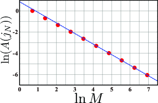
Figure 5: (Color online) The asymptotic amplitudes $A(n_{N})$ and $A(j_{N})$ of the local density $\langle n_{N}\rangle_{t}$ and current $\langle j_{N}\rangle_{t}$ plotted against the total number of sites $M$ for $M=2^{k},k=1,\cdots,10$.

Next, we make the scaling analysis of the asymptotic amplitudes $A(n_{k})$ and $A(j_{k})$ of the local densities $\langle n_{k}\rangle_{t}$ and currents $\langle j_{k}\rangle_{t}$. We take the amplitudes at the $N$-th site $A(n_{N})$ and $A(j_{N})$ as a representative. The top and bottom panel of Fig. 5 shows $\mathrm{ln}(A(n_{N}))\ \mathrm{vs}\ \mathrm{ln}M$ and $\mathrm{ln}(A(j_{N}))\ \mathrm{vs}\ \mathrm{ln}M$, respectively. The fitting from $M=256,512,1024$ gives $\mathrm{ln}(A(n_{N}))=1.937981-1.4933187\mathrm{ln}M$ and $\mathrm{ln}(A(j_{N}))=0.854409-0.9968579\mathrm{ln}M$. Confining to larger sites for fitting, the coefficient associated with $\mathrm{ln}M$ approaches to $-3/2$ and $-1$, which indicates $A(n_{N})\propto M^{-3/2}$ and $A(j_{N})\propto M^{-1}$ respectively.

Conclusions.$-$ In this article, we have studied the exact relaxation dynamics of the TASEP. We examined the behavior of the local densities and currents by use of the algebraic Bethe ansatz method. By quantitive evaluation, we see the convergence of the density and current profiles to the steady state densities and currents. Furthermore, we observe interesting behaviors such as the emergence of a ripple in the density profile and excessive flow of currents peculiar to the step initial condition. Moreover, by making a finite-size scaling analysis, we determine the scaling exponents of the asymptotic amplitudes of the local densities and currents with respect to the total number of sites, which are found to be $-3/2$ and $-1$ respectively.

The authors would like to thank C. Arita for useful discussions. The present research is partially supported by Grant-in-Aid for Young Scientists (B) No. 21740285. J.S. is supported by JSPS.

References

- (1) B. Derrida, Phys. Rep. 301 65 (1998).
- (2) G. Schütz, Exactly Solvable Models for Many-Body Systems Far from Equilibrium, Phase Transitions and Critical Phenomena Vol. 19 (Academic Press, London, 2000).
- (3) F. Spitzer, Adv. in Math. 5 246 (1970).
- (4) T.M. Liggett, Stochastic Interacting Systems: Contact, Vote, and Exclusion Processes, (Springer-Verlag, New York, 1999).
- (5) C.T. Macdonald, J.H. Gibbs and A.C. Pipkin, Biopolymers 6 1 (1968).
- (6) A. Schadschneider, Physica A 285 101 (2001).
- (7) A. Schadschneider, D. Chowdhury and K. Nishinari, Stochastic Transport in Complex Systems: From Molecules to Vehicles, (Elsevier Science, Amsterdam 2010).
- (8) T. Karzig and F. von Oppen, Phys. Rev. B 81 045317 (2010).
- (9) M. Kardar, G. Parisi and Y-C. Zhang, Phys. Rev. Lett. 56 889 (1986).
- (10) K.A. Takeuchi and M. Sano, Phys. Rev. Lett. 104 230601 (2010).
- (11) B. Derrida, M.R. Evans, V. Hakim and V. Pasquier, J. Phys. A 26 1493 (1993).
- (12) T. Sasamoto, J. Phys. A 32 7109 (1999)
- (13) R.A. Blythe, M.R. Evans, F. Colaiori and F.H.L. Essler, J. Phys. A 33 2313 (2000).
- (14) J. Krug, Phys. Rev. Lett. 67 1882 (1991).
- (15) D. Dhar, Phase Transitions 9 51 (1987).
- (16) L-H. Gwa and H. Spohn, Phys. Rev. A 46 844 (1992).
- (17) D. Kim, Phys. Rev. E 52 3512 (1995).
- (18) O. Golinelli and K. Mallick, J. Phys. A 37 3321 (2004); ibid 38 1419 (2005).
- (19) J. de Gier and F.H.L. Essler, Phys. Rev. Lett 95 240601 (2005).
- (20) J. de Gier and F.H.L. Essler, J. Stat. Mech P12011 (2006).
- (21) C. Arita, A. Kuniba, K. Sakai and T. Sawabe, J. Phys. A 42 345002 (2009).
- (22) K. Johansson, Comm. Math. Phys. 209 437 (2000).
- (23) M. Prähofer and H. Spohn, In and out of equilibrium, vol. 51 of Progress in Probability, 185-204, (Birkhauser, Boston, 2002)
- (24) A. Rakos, G.M. Schütz, J. Stat. Phys. 118 511 (2005).
- (25) T. Imamura and T. Sasamoto, J. Stat. Phys. 128 799 (2007).
- (26) C. Tracy and H. Widom, J. Math. Phys. 50 095204 (2009).
- (27) B. Derrida and J.L. Lebowitz, Phys. Rev. Lett. 80 209 (1998).
- (28) J. de Gier and F.H.L. Essler, Phys. Rev. Lett. 107 010602 (2011).
- (29) V.E. Korepin, N.M. Bogoliubov and A.G. Izergin, Quantum Inverse Scattering Method and Correlation functions (Cambridge University Press, 1993).
- (30) N.M. Bogoliubov, SIGMA 5 052 (2009).
- (31) J. Mossel and J-S. Caux, New J. Phys. 12 055028 (2010).