Constraints on Light Hidden Sector Gauge Bosons from Supernova Cooling
Abstract
We derive new bounds on hidden sector gauge bosons which could produce new energy loss mechanisms in supernovae, enlarging the excluded region in mass-coupling space by a significant factor compared to earlier estimates. Both considerations of trapping and possible decay of these particles need to be incorporated when determining such bounds, as does scattering on both neutrons and protons. For masses and couplings near the region which saturates current bounds, a significant background of such gauge bosons may also be produced due to the cumulative effects of all supernovae over cosmic history.
pacs:
95.35.+dI Introduction
Despite its phenomenological success, the Standard Model (SM) is known to be incomplete. Observations of neutrino masses and oscillations, and several naturalness issues (stability of the electroweak scale, strong CP problem) have motivated theoretical extensions, many of which involve the existence of new particles and forces. Extensions of the Standard Model by inclusion of one or more Abelian groups are familiar in a number of contexts. Additional groups naturally arise from the breaking of GUT groups to the Standard Model, from attempts to resolve the fine-tuning of the Higgs mass, or from the possible existence of new hidden sectors in nature (for a review see Jaeckel:2010ni ; Langacker:2008yv ). This latter alternative has elicited significant interest recently because it allows the possibility that new light gauge bosons associated with the new groups may connect a hidden sector to the observed sector, allowing for the existence of associated dark matter particles which may have enhanced couplings because of mixing between the new gauge bosons and photons.
If the boson were massless then it would mediate long-range forces, which would then necessitate a very small coupling to SM matter or that the new group be sequestered from the SM. Massive gauge bosons are not as strongly constrained, but even for additional sectors that are not charged under the SM there will still arise a coupling to the SM through kinetic mixing. That is, for a field strength with an associated gauge boson , and the hypercharge field strength , the Lagrangian density will contain the gauge invariant renormalizable terms Holdom:1985ag
| (1) |
If the is embedded in a GUT theory, Planck-suppressed operators or loop-suppressed mixing from heavy split multiplets can induce . In the context of string theory, the possible range of is much larger, with estimated values of from compactifications of the heterotic string, or in type II scenarios Dienes:1996zr ; Abel:2003ue ; Abel:2008ai ; Baumgart:2009tn . At low energies, the kinetic mixing can be removed by considering a shift in the photon field , inducing -suppressed electromagnetic interactions of the with strength :
| (2) |
where , with weak mixing angle .
As alluded to above, hidden sector models have garnered much attention recently because if there are dark matter particles in these sectors that are charged under a new dark gauge symmetry, the possibility exists for increased self interactions which could result, via mixing with the standard sector, in the possibility of an enhanced annihilation signature which was thought might explain anomalous cosmic ray data. Dark matter particles in the sector could have a mass at the weak scale, with the mass suppressed by down to the MeV-GeV scale (there exists a rather larger literature on such enhancements, see for example Padmanabhan:2005es ; Pospelov:2008jd ; ArkaniHamed:2008qn ; ArkaniHamed:2008qp ; Hisano:2008ti ; Hisano:2009rc ; Baumgart:2009tn ; Katz:2009qq ; Dent:2009bv ; Zavala:2009mi ; Feng:2009hw ; Buckley:2009in ; Slatyer:2009yq ; Feng:2010zp ; Finkbeiner:2010sm ; Hisano:2011dc ; Slatyer:2011kg ; Abazajian:2010zb ; Zavala:2011tt ; Abazajian:2011ak for models and constraints).
Of course, if the new gauge bosons are sufficiently light, they can also produce observable signatures, using direct and indirect terrestrial probes. Beam dumps, for example, which are sensitive to the possibility of new light penetrating particles such as axions provide stringent constraints Bjorken:2009mm ; Krauss:1986bw . In addition, one must consider the impact of new light gauge bosons on sensitive atomic probes such as the anomalous magnetic moment of the muon Pospelov:2008zw .
Supplementing these constraints on a hidden sector are constraints from astrophysics. If hidden sector gauge particles mix with photons and then escape from a star, then this new energy loss mechanism can dramatically affect not only stellar structure but also stellar evolution. Perhaps nowhere is this more dramatic than in the case of core collapse supernovae. As a result, supernova cooling constraints (namely the energy loss observed from SN1987a) have long been employed in order to constrain particle couplings and masses Iwamoto:1984ir ; Turner:1987by ; Brinkmann:1988vi ; Ellis:1988aa .
Early work was concerned principally with constraints on nearly massless axions emitted in nucleon-nucleon bremsstrahlung processes inside of the hot () neutron star born from an associated supernova. One can adapt this line of inquiry to constrain the masses and mixings of a hidden sector gauge boson, , which may couple to Standard Model-sector charged particles via the previously mentioned kinetic mixing. An estimate of the energy loss of such a process was given in Bjorken:2009mm , but, as is mentioned in that work, this estimate was expected to be accurate at best at the order of magnitude level.
It is the purpose of this work to provide a more thorough accounting of this process and thus derive more accurate constraints on the masses of such particles, , and their couplings, . Because models of interest for dark matter involve gauge boson masses which exceed MeV, we restrict ourselves to this range here. Moreover, for much lighter masses, other considerations arise. In particular, matter effects as particles traverse the high density collapsing core can be large enough to produce oscillation phenomena reminiscent of that for neutrinos which can cause enhanced trapping of such particles and thus may obviate the constraints we derive on heavier gauge bosons Redondo:2008aa . Dark matter particles in the sector are generically heavy and would not contribute to the cooling of the supernova. In scenarios where dark matter particles have masses below MeV, that could explain the 511 keV line emission from the galactic bulge Pospelov:2007mp ; Pospelov:2008jd ; Pospelov:2008zw , additional cooling channels could be present Mohapatra:1990vq ; Fayet:2006sa , which we do not consider below.
II Free Streaming
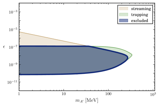
We are interested in exclusion regions in the plane. What one expects is that there will be an upper bound on above which the vector particle production will exceed the bounds from SN1987a, extending up to a value when the vector particles would be strongly enough coupled to be trapped inside the supernova core. This is what we will call the free streaming region. In the first sub-section we will outline calculations for the process , and then extend this to include the process as well.
II.1 The proton only case
The central quantity to calculate is the emission rate of the vector particles, which is labeled where the subscripts stand for the possible nucleons participating in the emission process. In the hot medium with temperature of a few MeV and densities typical of the accretion disk, the nucleons are nondegenerate and nonrelativistic. The main emission process is the nucleon-nucleon-dark boson bremsstrahlung. In studies of axion emission one usually neglects the mass of the emitted particle. Since our dark gauge boson can have a mass comparable to the temperature of the SN medium, this approximation is not justified and we follow the kinematical analysis of Giannotti:2005tn . The details of this somewhat lengthy calculation in the one-pion-exchange (OPE) approximation are given in the appendices. If we take the expression for given in Eq.(B.23), and use the fact that the couples to protons and charged pions with strength , we can write:
| (3) |
where denotes the phase space integration in terms of the dimensionless variables , and . We have also replaced the baryon number density, , by its mass density through . For the pion-nucleon coupling we take , resulting in in Eq. (3). In our calculations we will use the typical values and MeV for the density and temperature in the interior of a supernova. We then constrain the parameter space by imposing that the luminosity due to vector emission must be less than:
| (4) |
which is roughly the energy lost in neutrinos Raffelt:1996wa .
Since our expression for , Eq. (3), is the luminosity per unit volume, we need to integrate it over the volume where the vectors are emitted. We then assume that MeV holds within a central spherical region of 1 km in radius (if we take the SN to have a mass , then it would have a total radius of km assuming the same constant density).
Putting all this together, we find that the luminosity due to vector emission
| (5) |
cannot be larger than in Eq. (4).
So our constraint on the coupling can be written as:
| (6) |
and we then generate an exclusion bound with fixed, while varying for different masses . This will give an upper bound on the coupling in terms of .
II.2 Including neutron processes
Next we will include processes with both protons and neutrons. The expression for emission due to the process is given in Eq. (D.1). This situation is slightly more complicated as we now have five integrals contributing in the phase space integration. We can use Eq. (6) to find the limits, if we add a multiplicative factor of 8 in . This comes about as follows: there is a factor of from isospin requirements that the neutron-proton coupling to a charged pion is ; there is no longer a symmetry factor of , since proton and neutron are not indistinguishable; finally, we had a factor of 2 from in front of , but now . The results are shown in Fig. 1.
III Including decay
Naively, larger couplings that do not satisfy Eq. (6) would be excluded. But, the free streaming limit is not the only region in parameter space where constraints will arise. In general, due to the couplings in Eq. (2), the dark gauge boson decays back into leptons and other SM particles within a distance:
| (7) |
In order to implement this, we will follow the strategy outlined in Bjorken:2009mm and modulate the emission amplitude with an exponential damping factor,
| (8) |
The assumption is that the products of the decay remain within the SN core and do not contribute to the cooling 111This assumption might break in scenarios where can decay into hidden sector matter with a large branching ratio.. As the mixing parameter increases, the decay happens earlier and the gauge bosons are not effective at cooling, as seen in Fig. 1. Therefore we would expect that above some value of , the emission constraints will no longer hold, and we will find a lower bound on the coupling, creating a region bounded above and below once decay is included with free streaming.
This exponential factor enters the phase space integration, and as a result, the function becomes a function , but we can still use Eq. (6) with . When generating the plots, we took , which corresponds to the situation where only the decays are possible. We also take for the typical distance where decay products are trapped, and, as in the previous section, we assume that vector particles are produced within the inner km.
.
IV Trapping limit
Thus far we have examined the energy loss due to vectors which are emitted and subsequently decay outside of the supernova. However, as is well known, above a certain coupling, these particles can be trapped within the supernova. This will create a lower bound on the coupling , above which the trapping will not allow vector emission to contribute to cooling the supernova.
If the new particles generated in the nucleon interaction processes subsequently interact strongly enough they will thermalize, and will be emitted from a spherical shell where the optical depth is roughly . If the temperature is , the luminosity will be given by the Steffan-Boltzmann law:
| (10) |
Here is the Steffan-Boltzmann constant, which is for photons and
| (11) |
for a new particle with degrees of freedom.
In principle, one should determine and , but following Raffelt:1996wa we assume km. This is a good approximation, because the density of the protoneutron star falls abruptly near that radius.
The requirement that the luminosity in new particle emission be less than
| (12) |
translates into a bounded relation between the temperature and the coupling
| (13) |
To calculate one needs a model for the temperature and density above the settled inner SN core, for which we turn to Turner:1987by :
| (14) |
where , km, MeV, and is a relatively large number.
As shown below, given a model, the opacity can be expressed in terms of . It is then straightforward to compute the optical depth,
| (15) |
One then solves for from , and uses Eq. (14) to find . The temperature just found is used in Eq. (10) or compared to Eq. (13).
To find the opacity as a function of and , one starts from the reduced Rosseland mean opacity:
| (16) |
where we have used , the velocity , and the definition of is given by
| (17) |
Since the production of bosons involves a Bose stimulation factor, we need to add a factor of under the integral above. This gives the reduced opacity (often denoted as ), which is the one that we have been using. Dropping the superscript ∗, we find that:
| (18) |
which reduces to the expression for axions Raffelt:1996wa for , and .
In the corresponding calculation for a massless axion, the mean free path can be obtained as follows: starting from the energy-loss rate, , one removes the phase-space integral , and a factor of , since is an energy loss rate. Additionally a factor of must be included to account for the detailed-balance relationship, and this gives .
In our case, we have to take into account that the boson under consideration is massive. Therefore, the vector boson phase-space integral, is , with , and .
Hence, the inverse mean free path is obtained by removing from the luminosity, , the factor:
| (19) |
and adding the detailed balance term.
Our expression for is once again given by Eq. (B.23) for the case, and in Eq. (D.1) for the bremsstrahlung. We can write them both as follows:
| (20) |
where are functions defined in the appendix. The factor is equal to for scattering, and , with the usual isospin and non-identical particles enhancement in scattering.
Next, we perform the -integration with the help of the delta function, and we remove a factor of from the -phase-space integration. Additionally we must include the detailed balance term, which cancels an that appeared after the delta function was used.
Once all of these machinations are completed, the mean free path corresponding to each channel is found to be
| (21) |
We can now plug this expression into Eq. (18), and manipulate it to find
| (22) |
where we defined the dimensionless opacity:
| (23) |
and is defined above. We find the total contribution from both channels using the fact that inverse opacities add: .
One then defines the quantity . Substituting and in Eq. (22), we can find , and
| (24) |
Finally the opacity is found from Eq. (15) to be
| (25) |
This expression can now be used to bound the coupling as a function of the dark gauge boson mass by requiring . For the case considered in this section, of trapping without including decay, we find numerically the exclusion region shown in Fig. 1.
In a more realistic scenario one must take into account both trapping as well as decay. This will lead to an exclusion region which is the intersection of the regions from trapping and decay alone, as either process will ensure that no additional energy loss will occur. For small masses and stronger couplings, trapping constrains the excluded region of parameter space. Conversely, for larger masses and smaller couplings, decay becomes most important. The combined region is shown in Fig. 1.
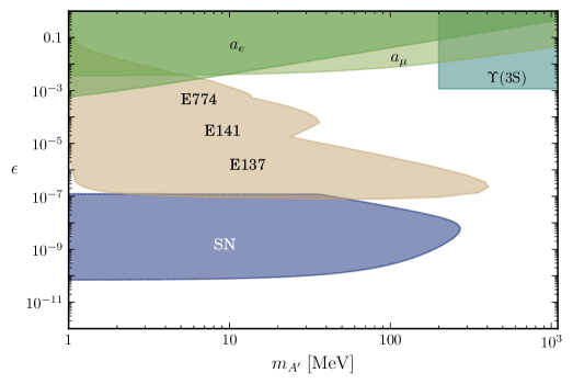
In Fig. 2 we display 222We thank J. Redondo for providing us with the non-supernova constraints shown in Fig. 2. the combined region along with constraints due to other sources such as beam dump experiments E774, E141, E137, contributions to the anomalous magnetic moment of the muon and the electron, and , and BABAR bounds from upsilon decays.
V A Diffuse Dark Gauge Boson Background?
With an average event rate of approximately yr-1 per galaxy, there have been over supernova explosions over cosmic history within our observable horizon. As was recognized even before SN1987a allowed more accurate estimate of neutrino production rates in supernova, and before recent supernova surveys allowed a more careful determination of event rates, the cumulative effect of such supernovae can produce a significant diffuse background of particles Krauss:1983zn . In particular a neutrino background in the MeV range with a flux in the range of cm-2sec-1 has been predicted. If a new dark gauge boson exists which is not ruled out by the arguments presented here, but which nevertheless contributes significantly to supernova cooling, a similar background of such particles would be expected. Indeed, similar considerations have recently been recognized for a possible diffuse axion background from supernovae Raffelt:2011ft . Because these particles are massive, the dominant contribution to energy loss will come from their mass as long as it exceeds the mean temperature near the surface of the supernova neutrinosphere. As a result we would expect a diffuse background today of dark gauge particles of mass as large as (MeV) cm-2sec-1. Their net contribution to the overall mass density of the universe would be negligible, but depending upon their interactions, such a background might be detectable. Moreover, if these particles are not stable, but decay into Standard Model particles, they would contribute to a diffuse cosmic ray background. We are therefore currently examining whether various direct and indirect constraints may be relevant for the possible detection of such a background inprogress .
VI Discussion
The calculations described here produce more accurate, and more importantly, significantly enhanced constraints on light gauge bosons that may arise from hidden sector models which predict novel types of dark matter. Mixing with photons produces results in bremsstrahlung production by scattering of both protons and neutrons, and a careful consideration of the resulting constraints from observations of SN1987a, involving both considerations of trapping and possible decay allow us to rule out a significantly larger region of masses and mixings than was previously estimated Bjorken:2009mm , extending a constraint on an effective coupling of less than for a significant range of gauge boson masses. We also note that for masses and mixings near those that saturate the supernova cooling bounds, a significant diffuse background of dark gauge bosons will be produced by the cumulative effects of all supernovae over cosmic history. Whether such a background might be detectable is of some interest, and is the subject of ongoing investigations.
VII Acknowledgements
We would like to thank H. Mathur, M. Ogilvie, J. Redondo, and T. Vachaspati for helpful discussions. LMK and JBD acknowledge support from the Department of Energy and Arizona State University. FF was supported in part by the U.S. DOE under Contract No. DE-FG02-91ER40628 and the NSF under Grant No. PHY-0855580.
Appendix A Amplitude for the process
Nucleon-nucleon bremsstrahlung is the primary mechanism for dark gauge boson emission from the inner core of the SN. Like in the corresponding axion calculation, we calculate the rate for this process in the one-pion-exchange (OPE) approximation, which is sufficiently reliable for our present purpose Turner:1989wa (although it could overestimate the emission rates by a small factor at lower temperatures Hanhart:2000ae ). Since the hidden sector boson only couples at tree level to SM particles with electric charge, we need only consider nucleon scattering processes which involve protons. We have eight diagrams for the OPE proton scattering processes with vector bremsstrahlung, and five diagrams for the process, where is the hidden sector gauge boson with mass , and we will take all nucleon masses to be . In this Appendix and in Appendix B we will examine the process , with a treatment of the process given beginning in Appendix C.
Following Brinkmann:1988vi these diagrams, as shown in Fig.(3), are designated , which gives a total of sixty-four terms from the squared matrix element
| (A.1) |
The plus sign is for the direct channel diagrams and the minus sign is for the exchange -channel diagrams. As required by gauge invariance, the amplitude satisfies
| (A.2) |
where represents the Feynmann amplitude without the external polarization vector.
The matrix elements for each diagram are given by
where is the coupling for the vertex, and we have used the momenta definitions and .
With these definitions we find the kinematic relations
As in previous work with massive axions Giannotti:2005tn , we will work in the approximation that the nucleon mass is much larger than both the temperature and the vector mass, and that the direct and exchange four-momenta transferred is larger than the vector mass and momenta, . This is due to the fact that the kinetic energy of the vector particles should roughly be a factor of a few times the temperature. We can then use the simplifying relation . Finally, we use the approximation , since .

Squaring the matrix elements, we find for the process
| (A.3) |
where , , and . Here the are the couplings between the and the ’th particle; which in this case is . Thus, will be the only non-zero contribution.
Appendix B Phase space integrations for the process
The energy emission rate is given by
| (B.1) |
where
| (B.2) |
The initial-state nucleon occupation numbers are given by the non-relativistic Maxwell-Boltzmann distribution
| (B.3) |
and is the symmetry factor, for the process and for the process. In the non-relativistic approximation, .
Following Brinkmann:1988vi ; Raffelt:1993ix ; Giannotti:2005tn we go to the center-of-momentum coordinates
| (B.4) | |||||
| (B.5) | |||||
| (B.6) | |||||
| (B.7) |
In the non-relativistic limit, a typical nucleon with kinetic energy has momentum . Then, the three dimensional delta function will enforce .
One defines the dimensionless variables
| (B.8) |
as well as , where is the angle between and . The velocity of the emitted boson, , can be written as
| (B.9) |
The momenta in Eq. (A.3) can then be written as
| (B.10) | |||||
| (B.11) | |||||
| (B.12) | |||||
| (B.13) | |||||
| (B.14) |
The delta function in the emission rate, Eq. (B.1), becomes
| (B.15) |
and we use the three-dimensional piece to do the integration.
We now change coordinate bases from , , to the , , system, including a factor of 8 (the inverse Jacobian).
Using
| (B.16) |
we obtain
| (B.17) | |||||
| (B.18) | |||||
| (B.19) |
Appendix C Amplitude for the process
The requisite matrix elements for the process are
| (C.1) | |||||
| (C.2) | |||||
| (C.3) | |||||
| (C.4) | |||||
| (C.5) |
where the coupling is the coupling for the vertex, which is related to as by isospin invariance. As in the case, is the coupling between the and the ’th particle. For this process we have .
The products of matrix elements for diagrams with bremsstrahlung originating off of external legs will produce terms in identical to those found in Appendix A for the process. However, we see that we will also find matrix element products which include the factor which arises from internal bremsstrahlung. These new combinations are given by
| (C.6) | |||||
| (C.7) | |||||
| (C.9) | |||||
| (C.12) | |||||
| (C.14) | |||||
| (C.16) |

Putting everything together we find
| (C.18) | |||||
where
| (C.19) | |||||
| (C.20) | |||||
| (C.21) | |||||
| (C.22) | |||||
| (C.23) |
Appendix D Phase Space Integrations for
We can now compute the phase space integrations in the same manner as in the case. We find
| (D.1) | |||||
| (D.2) |
where (note the dependence of the last four)
| (D.3) | |||||
References
- (1) J. Jaeckel and A. Ringwald, Ann.Rev.Nucl.Part.Sci. 60, 405 (2010), arXiv:1002.0329.
- (2) P. Langacker, Rev.Mod.Phys. 81, 1199 (2009), arXiv:0801.1345.
- (3) B. Holdom, Phys.Lett. B166, 196 (1986).
- (4) K. R. Dienes, C. F. Kolda, and J. March-Russell, Nucl.Phys. B492, 104 (1997), arXiv:hep-ph/9610479.
- (5) S. Abel and B. Schofield, Nucl.Phys. B685, 150 (2004), arXiv:hep-th/0311051.
- (6) S. Abel, M. Goodsell, J. Jaeckel, V. Khoze, and A. Ringwald, JHEP 0807, 124 (2008), arXiv:0803.1449.
- (7) M. Baumgart, C. Cheung, J. T. Ruderman, L.-T. Wang, and I. Yavin, JHEP 0904, 014 (2009), arXiv:0901.0283.
- (8) N. Padmanabhan and D. P. Finkbeiner, Phys.Rev. D72, 023508 (2005), arXiv:astro-ph/0503486.
- (9) M. Pospelov and A. Ritz, Phys.Lett. B671, 391 (2009), arXiv:0810.1502.
- (10) N. Arkani-Hamed, D. P. Finkbeiner, T. R. Slatyer, and N. Weiner, Phys.Rev. D79, 015014 (2009), arXiv:0810.0713.
- (11) N. Arkani-Hamed and N. Weiner, JHEP 0812, 104 (2008), arXiv:0810.0714.
- (12) J. Hisano, M. Kawasaki, K. Kohri, and K. Nakayama, Phys.Rev. D79, 063514 (2009), arXiv:0810.1892.
- (13) J. Hisano, M. Kawasaki, K. Kohri, T. Moroi, and K. Nakayama, Phys.Rev. D79, 083522 (2009), arXiv:0901.3582.
- (14) A. Katz and R. Sundrum, JHEP 0906, 003 (2009), arXiv:0902.3271.
- (15) J. B. Dent, S. Dutta, and R. J. Scherrer, Phys.Lett. B687, 275 (2010), arXiv:0909.4128.
- (16) J. Zavala, M. Vogelsberger, and S. D. White, Phys.Rev. D81, 083502 (2010), arXiv:0910.5221.
- (17) J. L. Feng, M. Kaplinghat, and H.-B. Yu, Phys.Rev.Lett. 104, 151301 (2010), arXiv:0911.0422.
- (18) M. R. Buckley and P. J. Fox, Phys.Rev. D81, 083522 (2010), arXiv:0911.3898.
- (19) T. R. Slatyer, N. Padmanabhan, and D. P. Finkbeiner, Phys.Rev. D80, 043526 (2009), arXiv:0906.1197.
- (20) J. L. Feng, M. Kaplinghat, and H.-B. Yu, Phys.Rev. D82, 083525 (2010), arXiv:1005.4678.
- (21) D. P. Finkbeiner, L. Goodenough, T. R. Slatyer, M. Vogelsberger, and N. Weiner, JCAP 1105, 002 (2011), arXiv:1011.3082.
- (22) J. Hisano et al., Phys.Rev. D83, 123511 (2011), arXiv:1102.4658.
- (23) T. R. Slatyer, N. Toro, and N. Weiner, (2011), arXiv:1107.3546.
- (24) K. N. Abazajian, S. Blanchet, and J. Harding, (2010), arXiv:1011.5090.
- (25) J. Zavala, M. Vogelsberger, T. R. Slatyer, A. Loeb, and V. Springel, Phys.Rev. D83, 123513 (2011), arXiv:1103.0776.
- (26) K. N. Abazajian and J. Harding, (2011), arXiv:1110.6151.
- (27) J. D. Bjorken, R. Essig, P. Schuster, and N. Toro, Phys.Rev. D80, 075018 (2009), arXiv:0906.0580.
- (28) L. M. Krauss and M. Zeller, Phys.Rev. D34, 3385 (1986).
- (29) M. Pospelov, Phys.Rev. D80, 095002 (2009), arXiv:0811.1030.
- (30) N. Iwamoto, Phys.Rev.Lett. 53, 1198 (1984).
- (31) M. S. Turner, Phys.Rev.Lett. 60, 1797 (1988).
- (32) R. P. Brinkmann and M. S. Turner, Phys.Rev. D38, 2338 (1988).
- (33) J. R. Ellis, K. A. Olive, S. Sarkar, and D. Sciama, Phys.Lett. B215, 404 (1988).
- (34) J. Redondo, JCAP 0807, 008 (2008), arXiv:0801.1527.
- (35) M. Pospelov, A. Ritz, and M. B. Voloshin, Phys.Lett. B662, 53 (2008), arXiv:0711.4866.
- (36) R. Mohapatra and I. Rothstein, Phys.Lett. B247, 593 (1990).
- (37) P. Fayet, D. Hooper, and G. Sigl, Phys.Rev.Lett. 96, 211302 (2006), arXiv:hep-ph/0602169.
- (38) M. Giannotti and F. Nesti, Phys.Rev. D72, 063005 (2005), arXiv:hep-ph/0505090.
- (39) G. Raffelt, Stars as laboratories for fundamental physics: The astrophysics of neutrinos, axions, and other weakly interacting particles (The University of Chicago Press, 1996).
- (40) L. M. Krauss, S. L. Glashow, and D. N. Schramm, Nature 310, 191 (1984).
- (41) G. G. Raffelt, J. Redondo, and N. V. Maira, (2011), arXiv:1110.6397.
- (42) J. B. Dent, F. Ferrer, and L. M. Krauss, in progress.
- (43) M. S. Turner, H.-S. Kang, and G. Steigman, (1989).
- (44) C. Hanhart, D. R. Phillips, and S. Reddy, Phys.Lett. B499, 9 (2001), arXiv:astro-ph/0003445.
- (45) G. Raffelt and D. Seckel, Phys.Rev. D52, 1780 (1995), arXiv:astro-ph/9312019.