RXTE Observations of Anomalous X-ray Pulsar 1E 1547.0$-$5408 During and After its 2008 and 2009 Outbursts

Abstract

We present the results of Rossi X-ray Timing Explorer (RXTE) and Swift monitoring observations of the magnetar 1E 1547.0$-$5408 following the pulsar’s radiative outbursts in 2008 October and 2009 January. We report on a study of the evolution of the timing properties and the pulsed flux from 2008 October 4 through 2009 December 26. In our timing study, a phase-coherent analysis shows that for the first 29 days following the 2008 outburst, there was a very fast increase in the magnitude of the rotational frequency derivative $\dot{\nu}$, such that $\ddot{\nu}$ was a factor of $\sim$ 60 larger than that reported in data from 2007. This $\dot{\nu}$ magnitude increase occurred in concert with the decay of the pulsed flux following the start of the 2008 event. Following the 2009 outburst, for the first 23 days, $\ddot{\nu}$ was consistent with zero, and $\dot{\nu}$ had returned to close to its 2007 value. In contrast to the 2008 event, the 2009 outburst showed a major increase in persistent flux, relatively little change in the pulsed flux, and sudden significant spectral hardening $\sim$15 days after the outburst. We show that, excluding the month following each of the outbursts, and because of the noise and the sparsity in the data, multiple plausible timing solutions fit the pulsar’s frequency behavior. We note similarities in the behavior of 1E 1547.0$-$5408 following the 2008 outburst to that seen in the AXP 1E 1048.1$-$5937 following its 2001-2002 outburst and discuss this in terms of the magnetar model.

1 Introduction

Anomalous X-ray Pulsars (AXPs) are young, isolated pulsars generally with a large inferred magnetic fields ($\gtrsim$ 10¹⁴ G). They are detected across the electromagnetic spectrum from the radio band (in 3 cases) to the hard X-ray regime. Like a closely related class of pulsars, the Soft Gamma Repeaters (SGRs), AXPs exhibit a wide range of variability, including but not limited to flux changes, spectral variability, X-ray bursts, X-ray flares, pulse profile changes, timing glitches, and rapid changes in the rotational frequency derivative. AXPs and SGRs are generally believed to be forms of magnetars. The magnetar model (Thompson & Duncan, 1995, 1996; Thompson et al., 2002) identifies the power source of these objects to be the decay of their strong magnetic fields. Most of the known magnetars have been observed to have entered an active phase at least once in the past, during which one or more of the listed types of variability was observed. For recent reviews, see Kaspi (2007), Mereghetti (2008), or Rea & Esposito (2011).

The X-ray source 1E 1547.0$-$5408 was discovered in 1980 with the Einstein satellite during a search for X-ray counterparts of unidentified X-ray sources (Lamb & Markert, 1981). It was first proposed to be a magnetar by Gelfand & Gaensler (2007) who showed that the spectrum was well described by a blackbody plus power-law model, typical of AXPs, and that the source is located at the center of a radio shell which is possibly a previously unidentified supernova remnant.

Since its discovery, the source has exhibited many X-ray flux variations (see Bernardini et al., 2011, for a review). First, a comparison of the X-ray flux of 1E 1547.0$-$5408 between 1980 and 2006 observed by Einstein, ASCA, XMM, and Chandra done by Gelfand & Gaensler (2007) revealed that the source’s absorbed 0.5$-$10 keV X-ray flux decreased during this period by a factor of $\sim$ 7. Then, analysis of Swift data taken in 2007 June and presented in Camilo et al. (2007) showed that the source’s X-ray flux was $\sim$3 times higher than the highest historic level and $\sim$16 times higher than the lowest level.

Camilo et al. (2007) observed 1E 1547.0$-$5408 in the radio band and detected pulsations at a period of $\sim$ 2.069 s, the smallest yet seen in a magnetar. The detected pulse profile was much wider than those of most rotation-powered long-period pulsars, and it was highly variable. Camilo et al. also estimated $\dot{P}$ to be 2$\times$10^-11, which, together with the value of $P$, imply a magnetar strength field (assuming $B\equiv 3.2\times 10^{19}$ G$\sqrt{P\dot{P}}$) of $2.2\times 10^{14}$ G), and furthermore that this is the magnetar with the largest $|\dot{\nu}|$ yet known.

Following the discovery of radio pulsations, Halpern et al. (2008) studied the X-ray emission of 1E 1547.0$-$5408 from 2007 June to 2007 October with Swift and XMM. They showed that the X-ray flux faded by about $\sim$ 50% from June to August. It subsequently stabilized. This suggests that an X-ray outburst occurred prior to 2007 June. Halpern et al. also detected faint X-ray pulsations for the first time with XMM. Moreover, during this period of time, a radio timing analysis showed that the pulsar’s $\dot{\nu}$ had systematically decreased by $\sim$25% (Camilo et al., 2008).

In 2008 October, 1E 1547.0$-$5408 entered a new active phase. The Swift BAT instrument detected several soft ($<$ 100 keV) bursts from the location of 1E 1547.0$-$5408 (Israel et al., 2010). An analysis of X-ray data from a variety of telescopes following the burst showed that the source was $>$50 times brighter than the lowest reported level and that the spectrum was significantly harder (Israel et al., 2010; Kaneko et al., 2010; Ng et al., 2011). The data further showed X-ray pulsations and a frequency derivative more negative –and changing – compared with the value reported in the radio data in 2007.

The source entered a second, even more active phase in 2009 January (Mereghetti et al., 2009; Kaneko et al., 2010) during which a large number of soft gamma-ray bursts was observed, as were well defined dust-scattering rings (Tiengo et al., 2010). Enoto et al. (2010a) reported the discovery of a hard X-ray tail just after the outburst using Suzaku, a result corroborated by Bernardini et al. (2011). A detailed analysis of the bursts detected with Swift after 2009 January outburst is presented by Scholz & Kaspi (2011), in addition to an analysis of the Swift persistent and pulsed flux data taken immediately following the initial trigger, showing that the source’s flux rose for 6 hrs following the trigger.

A comparison of the 2008 and 2009 events showed interesting differences. The former showed a large pulsed flux increase whereas the latter, though having an enormous persistent flux increase, showed only a modest pulsed flux increase. Ng et al. (2011) pointed out, in part using data reported on in this work, that the spectral variations in Chandra observations of the two epochs were similar, in contrast to very different $\dot{\nu}$ behaviors (see §3). They also noted a significant pulsed fraction/flux anti-correlation. Bernardini et al. (2011) reported on data from INTEGRAL, XMM-Newton, and the Chandra X-ray Observatory, finding similar $\dot{\nu}$, flux and spectral results. They summarize the source’s flux behavior since 1980 and argue it shows three well-defined flux ‘states.’

Here we present a detailed analysis of RXTE monitoring observations of 1E 1547.0$-$5408 following its 2008 October and 2009 January outbursts, supplemented by multiple Swift observations obtained during the same time period. We report the results of an in-depth analysis of the timing behavior, pulsed flux changes, and pulse profile variations. Our observations are described in Section 2. Our timing, pulse morphology, and pulsed flux and hardness ratio analyses are presented, respectively, in Sections 3, 4, and 5.

2 Observations and Pre-Analysis

2.1 RXTE Observations

The results presented here were obtained using the proportional counter array (PCA) on board RXTE. The PCA consists of an array of five collimated xenon/methane multi-anode proportional counter units (PCUs) operating in the 2$-$60 keV range, with a total effective area of approximately 6500 cm² and a field of view of $\sim$1^∘ FWHM (Jahoda et al., 1996).

For this paper, we used 114 RXTE observations. Of these, 49 observations were taken between 2008 October 4 and 2009 January 14, following the 2008 October outburst, and 65 observations were taken between 2009 January 22 and 2009 December 26, following the 2009 January outburst. The length of the observations varied between 0.6 ks and 17 ks, but most were between 1 ks and 6 ks. The epochs of the observations are shown in Figure 1. Notice the high density of observations in the first few days following each outburst.

Table 1 contains a list of the 49 observations obtained after the 2008 October outburst, showing the observation date, length, number of PCUs on, the type of analysis that each observation was used for, and the number of bursts found using the burst search algorithm introduced in Gavriil et al. (2002) and discussed further in Gavriil et al. (2004). Table 2 contains a similar list of the 65 observations subsequent to the 2009 January outburst.

For all observations, data were collected using the GoodXenon mode. This data mode records photon arrival times with 1-$\mu$s resolution and bins photon energies into one of 256 channels. To maximize the signal-to-noise ratio, we analysed only the events from the top Xenon layer of each PCU.

For each observation, we adjusted photon arrival times at each epoch to the solar system barycenter, using the source position given in Gelfand & Gaensler (2007) ($\alpha$_J2000=15:50:54.11 $\delta$_J2000=$-$54:18:23.7). Then, for each observation, we extracted a time series binned at a resolution of 1/32 s, in the 2$-$6.5 keV range (to maximize the signal to noise ratio), which utilized all PCUs, to be used in the timing and pulse profile analysis. Also for each observation, we extracted time series in various energy ranges, binned at the same time resolution, but excluding PCUs 0 and 1 because of the loss of their propane layers, to be used for the pulsed flux, pulse profile, and hardness ratio analyses. For each of the generated time series, 7-s long intervals of data were removed around large bursts. We verified that 7-s was sufficiently long. A large burst was defined to be any with count rate greater than or equal to 50 counts s^-1 PCU^-1 at the peak.

2.2 Swift Observations

In this paper, Swift observations were used uniquely for timing purposes. We used all 16 observations taken between 2008 October 03 and 2009 January 12, 14 of which were taken in the month following the onset of the 2008 outburst, and the remaining 2 taken in 2009 January, see Figure 1. We also used 8 Swift observations taken in the 23 days following the onset of the 2009 outburst, and all observations taken between 2009 February 13 and 2009 December 26 that were long enough to yield a clear pulse profile. Table 3 contains a list of the Swift observations used in this work, all of which were in Windowed Timing (WT) mode.

For each observation, we extracted photons from a 40-pixel-long strip centered on the source, and we adjusted the photon arrival times of each epoch to the solar system barycenter. Then, for each observation, we extracted a time series binned at a resolution of 1/32 s in the 2$-$7 keV range, to match the RXTE band.

3 Phase-Coherent Timing

Time series for all 95 RXTE observations having a sufficiently high signal-to-noise ratio were divided in half and treated as two separate time series. Time series for all 32 Swift observations were not divided. Each time series was epoch-folded using an ephemeris determined iteratively by maintaining phase coherence as we describe below. When an ephemeris was not available, we folded the time series using a frequency obtained from a periodogram. Resulting pulse profiles, with 64 phase bins, were cross-correlated in the Fourier domain with a high signal-to-noise-ratio template created by adding phase-aligned profiles. The cross-correlation returned an average pulse time-of-arrival (TOA) for each observation, corresponding to a fixed pulse phase.

The pulse phase $\phi$ at any time $t$ can usually be expressed as a Taylor expansion,

$$\phi(t)=\phi_{0}(t_{0})+\nu_{0}(t-t_{0})+\frac{1}{2}\dot{\nu_{0}}(t-t_{0})^{2}+\frac{1}{6}\ddot{\nu_{0}}(t-t_{0})^{3}+{\ldots},$$ (1)

where $\nu$ $\equiv$ 1/$P$ is the pulse frequency, $\dot{\nu}$ $\equiv$ $d\nu$/$dt$, etc., and subscript “0” denotes a parameter evaluated at the reference epoch $t=t_{0}$.

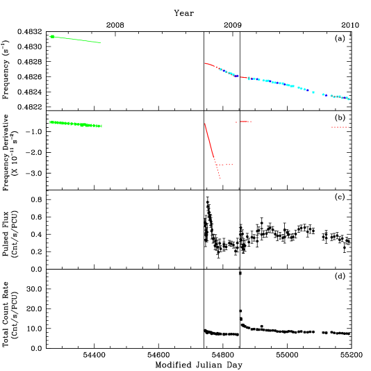
Figure 2: Long-term evolution of 1E 1547.0$-$5408 properties. (a) Frequency as a function of time. Green square: frequency from radio data (Camilo et al., 2007). Green line: evolution of the frequency $\nu$ as a quadratic polynomial where ${\nu}_{o}$ and ${\dot{\nu}}_{o}$ are obtained from Camilo et al. (2007), and ${\ddot{\nu}}$ is from the best-fit slope to Panel 2 of Figure 6 in Camilo et al. (2008). Red solid lines: frequency as a function of time from phase-coherent timing. Red dotted lines: possible but not unique phase-coherent solutions. Dark blue points: individual frequency measurements, each obtained from a combination of closely spaced observations. Light blue points: individual frequency measurements, each obtained from a long observation. (b) Frequency derivative as a function of time. Green points: $\dot{\nu}$ measurements taken from Camilo et al. (2008). Red solid lines: $\dot{\nu}$ as a function of time from phase-coherent timing. Red dotted lines: possible but not unique phase-coherent solutions. (c) Pulsed flux in the 2$-$10 keV band. (d) Count rate in the 2$-$10 keV band from the full RXTE field of view. All panels: the two solid vertical lines mark the onset of the two outbursts.

To obtain ephemerides for the time periods following each outburst, we fitted the TOAs to the above polynomial using the pulsar timing software package TEMPO. Since the spin-down of this source was unstable, and since consecutive observations were not always sufficiently close to each other, phase coherence could only be unambiguously maintained for a period of 29 days following the first outburst, and 23 days following the second outburst. The two timing solutions found are represented by solid red lines in the first two panels of Figure 2, along with the radio timing parameters of the same source from 2007 (Camilo et al., 2007, 2008). The spin parameters for these two timing solutions are shown in Table 4. The 2008 and 2009 ephemerides are consistent within 2$\sigma$ with those reported in Israel et al. (2010) and in Bernardini et al. (2011), although they extend for a few days longer than in the previous analyses.

We made various attempts at finding the pulsar frequency outside of these time periods. First, for each instance where closely spaced RXTE observations were available, a frequency measurement was found by doing TEMPO fits through the closely spaced TOAs. These frequency measurements are shown as dark blue points in the first panel of Figure 2.

Then, all 29 observations longer than 5.5 ks were broken into 2 or 3 fragments, TOAs were extracted for each fragment, and a frequency measurement was found for each long observation by fitting a linear trend to the phases with TEMPO. These frequency measurements are shown as light blue points in the first panel of Figure 2.

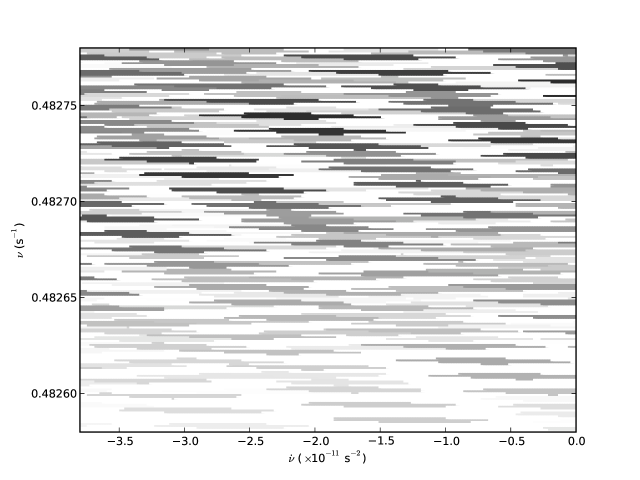
Figure 3: Results of the search for a phase-coherent timing solution consisting of a frequency $\nu$ and of a single frequency derivative $\dot{\nu}$ for a set of TOAs covering a time period of 11 days, and starting 21 days after the onset of the first outburst (MJD 54764.846 to 54775.050). The x-axis shows trial $\dot{\nu}$ values. The y-axis shows trial $\nu$ values. For every pair of $\nu$ and $\dot{\nu}$, the shading corresponds to the reduced ${\chi}^{2}$ obtained when the pair was used as set of trial phase-coherent timing parameters by TEMPO. White squares correspond to a reduced ${\chi}^{2}$ of 6 and above. Black squares correspond to a reduced ${\chi}^{2}$ of 0. The center of each of the uniformly-shaded islands corresponds to the best-fit $\nu$ and $\dot{\nu}$ found by TEMPO for each point on that island, and the size of each island corresponds to the uncertainty on the obtained $\nu$ and $\dot{\nu}$. The presence of several black islands clearly indicates the presence of several plausible timing solutions differing from each other by a small number of phase counts.

We also made several attempts at finding phase-coherent timing solutions outside the one month following each outburst. We broke the list of all TOAs (one or two TOAs per observation) into 69 overlapping sets of TOAs. For each set of TOAs, we searched for a phase-coherent timing solution by running a TEMPO fit for every plausible combination of $\nu$ and $\dot{\nu}$. The results of the search of one such set of TOAs are presented in Figure 3. For each guess combination of $\nu$ and $\dot{\nu}$, TEMPO returned a best-fit $\nu$ and $\dot{\nu}$, and timing residuals from which a reduced ${\chi}^{2}$ was extracted and represented as a shade in Figure 3, with the darker shade corresponding to a smaller reduced $\chi^{2}$. Note the appearance of several “islands” on the Figure. The center of each island corresponds to the best-fit $\nu$ and $\dot{\nu}$ returned by TEMPO.

The fact that many islands appear in the Figure indicates that any timing solution found to cover the time period spanned by the set of TOAs is not unique. Instead, the various islands correspond to several plausible timing solutions, differing from each other by a small number of pulse phases.

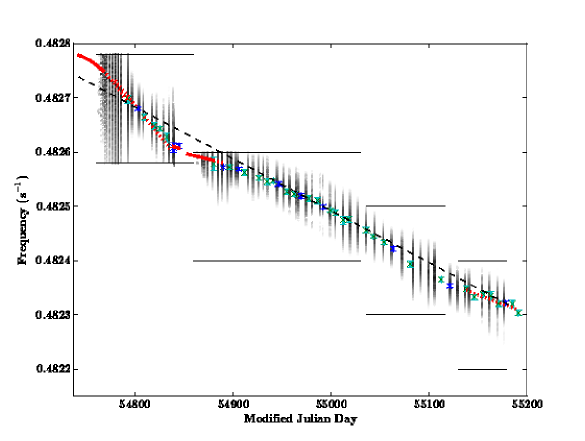
Figure 4: Frequency as a function of time for 1E 1547.0$-$5408. Shaded black columns: each of the black columns corresponds to one of the overlapping sets of TOAs. The x-coordinate of the column corresponds to the time in the middle of that set of TOAs. Every column was obtained by collapsing vertically a rectangle similar to that shown in Figure 3. The shading of each square in every shaded column appearing in this Figure corresponds to the darkest shading in the corresponding row in a $\nu$ and $\dot{\nu}$ map similar to that shown in Figure 3, and represents the best-fit reduced ${\chi}^{2}$. The presence of several black squares in every column indicates the presence of several plausible phase-coherent timing solutions at each epoch. The black horizontal lines represent the limits of the searched frequency values. The red solid lines represent frequency as a function of time from phase-coherent timing. The red dotted lines represent possible but not unique phase-coherent solutions. The dark blue points represent individual frequency measurements, each obtained from a set of closely spaced observations. The light blue points represent individual frequency measurements, each obtained from a long observation. The dashed line is an eyeball fit to all frequency measurements from 2008 and 2009. The two vertical black lines denote the onset of the two outbursts.

Once a shaded $\nu$ and $\dot{\nu}$ map, like that shown in Figure 3, was obtained for each overlapping set of TOAs, we collapsed each map, in the horizontal direction, into a single shaded column. The shade at each height of the column corresponds to the darkest shade in the corresponding row of the original $\nu$ and $\dot{\nu}$ map before the collapse. We then plotted all the shaded columns in Figure 4, along with the various phase-connected timing solutions and along with the individual frequency measurements.

For the columns near the outbursts, the number of dark spots in each shaded column was small, indicating a small number of possible phase-connected timing solutions. However, the fact that the number of dark regions in each shaded column increased as we got further from the outbursts clearly indicates that timing solutions found outside of the time periods covering the month following each outburst are not unique. Some of the longest-running non-unique solutions are shown as dotted red lines in Figures 2 and  4. In the 2008 event, the loss of phase-coherence is almost certainly due to enhanced timing noise in the pulsar as the frequency of observations had not significantly dropped when phase coherence was lost; in the 2009 event, the time interval between observations was somewhat larger when phase coherence was lost, although the coincidence of the loss and the decay of the persistent flux suggests the source behavior plays an important role.

4 Pulse Profile Analysis

First, for each RXTE observation, we folded the data in the 2–6.5 keV band using the best-fit frequency found in the timing analysis (Section 3). We then cross-correlated the resulting profile with a standard template in order to obtain phase-aligned profiles.

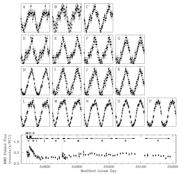
Figure 5: Normalized 2$-$6.5 keV pulse profiles of 1E 1547.0$-$5408 from 2008 October to 2010 December. Two cycles per plot are shown for clarity. The letter shown in the top-left corner of each plot refers to the time segments marked by arrows in the bottom plot, where the 2$-$10 keV RMS pulsed flux is shown for reference. The profiles marked with the letters A, B, and D to G are obtained from individual observations. The first and third dotted lines in the bottom plot correspond to the onsets of the two outbursts.

We then divided the period following the first outburst (3 October to 22 January) into intervals with similar net exposures, shown with the letters A through K at the bottom of Figure 5. We did the same for the period following the second outburst (22 January to 26 December 26); the intervals are shown with the letters L through P at the bottom of Figure 5.

For each time interval, we summed the aligned profiles, subtracted the DC component, and scaled the resulting profile so that the value of the highest bin is unity and the lowest point is zero. The results are presented in Figure 5 with the time intervals marked in the top left corner of each profile. The different profile qualities are due to the changes in the pulsed flux of the pulsar. Nevertheless, clear changes in pulse morphology are apparent. For example, the profile peak is clearly narrower immediately following the second 2008 pulsed flux enhancement, and shows the full width, but is more flat-topped following the 2009 outburst. The results shown here are generally consistent with those of Ng et al. (2011) and Bernardini et al. (2011).

Note however that in no case are any pulse profile changes so large that the profile peak, the assumed fiducial point, cannot be unambiguously identified. This is in contrast to other examples of AXP outbursts in which multiple peaks appeared, rendering unambiguous pulse numbering problematic (e.g. Woods et al., 2011). This gives us confidence that the timing analysis reported in the previous Section, in particular the difficulties phase-connecting the timing data, are not significantly affected by pulse profile changes. Indeed the epochs in which the profile changes are largest (namely immediately following the outbursts) are those which we have successfully phase-connected.

To study the evolution of the pulse profile with energy, we repeated the above analysis for energy bands 2$-$4 keV, 4$-$10 keV, and 2$-$10 keV. Figure 6 shows the evolution of the pulsed flux with energy for time intervals M and N indicated at the bottom of Figure 5. Note that the location of the peak of the profile seems to be energy-dependent, with the peak more to the left at higher energies, and more to the right at lower energies. This implies that spectral changes might cause slight shifts in the location of the pulse peak in the energy band used for the timing analysis (2$-$6.5 keV), but again, not large enough to cause a loss in pulse counting. Also note that pulse profiles at higher energies are not shown because of the very poor signal-to-noise ratio at these energies.

5 Pulsed Flux Time Series and Hardness Ratios

To obtain the pulsed flux for 1E 1547.0$-$5408, for each observation, we folded the data and extracted aligned pulse profiles in several energy bands. For each folded profile, we calculated the RMS pulsed flux,

$$F_{RMS}={\sqrt{2{\sum_{k=1}^{n}}(({a_{k}}^{2}+{b_{k}}^{2})-({\sigma_{a_{k}}}^{2}+{\sigma_{b_{k}}}^{2}))}},$$ (2)

where $a_{k}$ is the $k^{\textrm{\small{th}}}$ even Fourier component defined as $a_{k}$ = $\frac{1}{N}{\sum_{i=1}^{N}}{p_{i}}\cos{(2\pi ki/N})$, ${\sigma_{a_{k}}}^{2}$ is the variance of $a_{k}$, $b_{k}$ is the odd $k^{\textrm{\small{th}}}$ Fourier component defined as $b_{k}$ = $\frac{1}{N}{\sum_{i=1}^{N}}{p_{i}}\sin{(2\pi ki/N})$, ${\sigma_{b_{k}}}^{2}$ is the variance of $b_{k}$, $i$ refers to the phase bin, $N$ is the total number of phase bins, $p_{i}$ is the count rate in the $i^{\textrm{\small{th}}}$ phase bin of the pulse profile, and $n$ is the maximum number of Fourier harmonics used; here $n$=4.

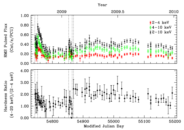
Figure 7: Pulsed flux time series and pulsed hardness ratio of 1E 1547.0$-$5408. Top: evolution of the RMS pulsed flux of 1E 1547.0$-$5408 in 2$-$4 keV, 4$-$10 keV, and 2$-$10 keV. Note the latter time series was shown by Ng et al. (2011) and Scholz & Kaspi (2011). Bottom: The hardness ratio as a function of time, computed from the ratio of pulsed fluxes in the energy range 4$-$20 keV to 2$-$4 keV. All panels: The first dotted line marks the onset of the first outburst. The second dotted line marks the location of an enhancement in the pulsed flux. The third line marks the onset of the second outburst. The last two dotted lines bracket the time interval inside which the hardness ratio rose.

In the top panel of Figure 7, we show the RMS pulsed flux in 2$-$10 keV, 2$-$4 keV, and in 4$-$10 keV. Note the 2$-$10 keV time series was previously shown by Ng et al. (2011) and Scholz & Kaspi (2011). The panel shows a slow decrease in the pulsed flux after the first outburst interrupted by a spike 9 days after the outburst. The spike was followed by a slow decrease. The source behaves differently after the second outburst, when the persistent flux increases dramatically (Figure 2d) while the pulsed flux does not vary significantly, implying a large decrease in the pulsed fraction following the second outburst. This is consistent with results of Ng et al. (2011), Bernardini et al. (2011), and Scholz & Kaspi (2011).

In the bottom panel of Figure 7, we show the hardness ratio as a function of time, computed from ratio of the pulsed fluxes in the energy ranges 4$-$20 keV to 2$-$4 keV. The Figure shows a clear discontinuity in the pulsed hardness ratio $\sim$ 15 days after the outburst, in the time period bracketed by the last two dotted lines, which, notably, is subsequent to the bulk of the pulsed flux decay, but while the persistent flux was still relatively high. We also computed the hardness ratio in various other energy bands, but the discontinuity was most significant for the energy range shown. Unfortunately Suzaku (Enoto et al., 2010a) and INTEGRAL (Bernardini et al., 2011) hard X-ray observations of the source both occurred prior to the hardness change seen with RXTE.

6 Discussion

The behavior of 1E 1547.0$-$5408 over the past several years has been extremely complex, indeed mirroring the complexity of the behaviors of AXPs in outburst in general. In a collection of detailed analyses of various X-ray and gamma-ray data sets (Israel et al., 2010; Kaneko et al., 2010; Ng et al., 2011; Scholz & Kaspi, 2011; Bernardini et al., 2011), including the present RXTE study reported on herein, a picture emerges of dramatic and varied multiwavelength behavior, including at least two very different outbursts from this intriguing source, albeit bearing some common properties. In the latter category is the generic X-ray hardness/flux correlation seen now commonly in magnetar outbursts (see Rea & Esposito, 2011; Scholz & Kaspi, 2011, for reviews), X-ray pulse profile changes, and ubiquitous X-ray bursting near outburst epochs, and significant changes in spin-down rate at and surrounding outburst epochs. We focus on this latter point here.

Magnetar rotational evolution during and near radiative outbursts has shown a wide range of behaviours, including large spin-up glitches with unusual recoveries (e.g. Kaspi et al., 2003), likely spin-down events (e.g. Palmer, 2002; Woods et al., 2002), initial spin-up events paired with large over-recovery, yielding net spin-down (Livingstone et al., 2010), and large $\dot{\nu}$ variations on week-to-month time scales (Gavriil & Kaspi, 2004; Dib et al., 2009). We note that throughout, no AXP has ever been observed to spin up for an extended period of any duration; only changes in magnitude in the spin-down rate punctuated by occasional, sudden, unresolved spin-up events have yet been observed. This is in stark contrast to behavior generally seen in accreting systems (e.g. Chakrabarty et al., 1997). Nevertheless, the diversity in magnetar rotational evolutions near the epochs of radiative outbursts has been perplexing.

However, we note that the behavior of 1E 1547.0$-$5408 following its 2008 outburst is reminiscent of unusual timing evolution seen thus far uniquely in AXP 1E 1048.1$-$5937 following its 2002 flux ‘flare’ (Gavriil & Kaspi, 2004; Dib et al., 2009). We compare the two next.

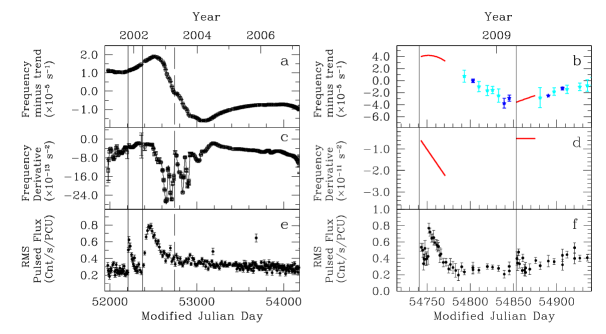
Figure 8: Comparison of the timing and pulsed flux properties of 1E 1048.1$-$5937 (left column) and 1E 1547.0$-$5408 (right column). (a) Frequency as a function of time for 1E 1048.1$-$5937 with a linear trend subtracted (for details, see Figures 3 and 15 of Dib et al. 2009). (b) Frequency as a function of time for 1E 1547.0$-$5408 with a linear trend subtracted (see Figure 2 for details). (c) Frequency derivative as a function of time for 1E 1048.1$-$5937. (d) Frequency derivative as a function of time for 1E 1547.0$-$5408. (e) Pulsed flux as a function of time in the 2$-$10 keV band for 1E 1048.1$-$5937. (f) Pulsed flux as a function of time in the 2$-$10 keV band for 1E 1547.0$-$5408.

In the case of 1E 1048.1$-$5937, the pulsar’s pulsed flux had been relatively stable in several years of RXTE monitoring, when a small (factor of $\sim$2) pulsed flux increase was observed near the end of 2001 (see Fig. 8e), accompanied by short SGR-like bursts (Gavriil et al., 2002) and pulse profile changes (Dib et al., 2009). The pulsed flux relaxed back to near quiescence in $\sim$3 weeks, but then there was a second, larger pulsed flux increase, this time by a factor of $\sim$3 over the span of a few weeks. This larger pulsed flux ‘flare’ subsequently decayed on a time scale of several months. This latter decay occurred just prior to an increase in the magnitude of $\dot{\nu}$, by over an order of magnitude (Fig. 8c). During both flares, the pulsar suffered significant pulse profile changes, the largest of which were at the flare peak, with the pulse relaxing back on approximately the same time scale as the pulsed flux dropped. Subsequently, there was a $\sim$2-yr period of large variations in $\dot{\nu}$, which while always remaining negative, varied by as much as an order of magnitude on time scales of a few weeks (see Fig. 15 in Dib et al. 2009; Fig. 8c). Phase connection in this extremely noisy interval was difficult, but enabled by extremely frequent RXTE observations – approximately three per 7–10-day interval.

The 2008 outburst of 1E 1547.0$-$5408 showed similar behavior (Fig. 8). The pulsed flux was clearly enhanced in our RXTE observations, which were triggered by SGR-like bursts. This enhancement then started to relax, but the decay was interrupted by a second pulsed flux increase $\sim$2 weeks later, this time by a factor of $\sim$4, similar to the increase in the pulsed flux in the second 2002 flare of 1E 1048.1$-$5937 (compare Fig. 8e and f). The pulse profile changed, particularly near the peak of the second ‘flare.’ Moreover, $\dot{\nu}$, as for 1E 1048.1$-$5937, dropped by a factor of $\sim$4, but roughly in concert with the pulsed flux decrease, before phase-coherence was lost (Fig. 8d). It is plausible that large $\dot{\nu}$ variations ensued, but we cannot unambiguously confirm this as the spacing of subsequent RXTE and Swift observations was not as dense as for 1E 1048.1$-$5937. Clearly though, $\dot{\nu}$ recovered to its 2007 value by the time of the 2009 outburst, so another dramatic change must have occurred.

Thus, the behavior of 1E 1547.0$-$5408 during its 2008 outburst is similar to that of 1E 1048.1$-$5937 in 2001-2002, as suggested in Figure 8: in both cases there was an initial, smaller flare accompanied by bursting, and a much larger flare a few weeks later. In both cases, the flares were accompanied by pulse profile changes in which the largest changes occurred near the peaks of the flares. Then, importantly, a pulsed flux decay occurred near or simultaneous with an increase in the magnitude of $\dot{\nu}$ by a factor of $\sim$4, followed by a very noisy period, in which regular phase-coherent timing was impossible. We note these similarities exist in spite of the fact that 1E 1048.1$-$5937 is a persistent, bright AXP, while 1E 1547.0$-$5408 has the properties of a transient AXP.

Note however that this behavior was not replicated in the 2009 1E 1547.0$-$5408 outburst: in that case $\dot{\nu}$ remained close to that reported in the radio data by Camilo et al. (2007). Also, in the 2009 outburst, the pulsed flux was barely affected, while the persistent flux increased by an order of magnitude (Fig. 2). Still, phase-coherence became again impossible some 23 days after the 2009 outburst. We note low-level but significant pulsed flux variations subsequently, which could be relevant.

The similarity between the 2008 outburst of 1E 1547.0$-$5408 and the 2001-2002 outburst of 1E 1048.1$-$5937 is potentially interesting. In the magnetar model, large flux enhancements are easy to envision given the great stresses placed on the crust due to internal magnetic field decay. Moreover, field-line distortions in the magnetosphere are expected as the crust shifts and the magnetosphere twists, hence pulse profile changes are also generically expected. Beloborodov (2009) argues that magnetospheric twists will impact the pulsar spin-down in two possible ways. One is that a strong twist results in an enhancement of the poloidal field lines, which leads to a stronger spin-down torque on the star (Thompson et al., 2002). This enhanced $\dot{\nu}$ is then expected to decay back to the standard value. The second way is that once the twist angle $\psi$ reaches a maximum value, it “boils over,” with energy that would have been stored in the magnetosphere had $\psi$ continued to increase being carried away by an intermittent magnetic outflow, which can carry away significant angular momentum. In this picture, any delay between such intermittent magnetic outflows and the outburst onset is due to the time it takes $\psi$ to reach its maximal value, though the increase in $\dot{\nu}$ is expected to commence much earlier (Beloborodov, 2009).

While the torque variations picture put forth by Beloborodov (2009) may provide a qualitative explanation of the behavior we have seen in the 2001-2002 outburst of 1E 1048.1$-$5937 and the 2008 outburst of 1E 1547.0$-$5408, it remains to be seen if the model can explain quantitatively the large $\dot{\nu}$ variations observed unambiguously for 1E 1048.1$-$5937, namely order-of-magnitude magnitude changes. Indeed the magnitude of the initial torque increase for strong ($\psi>1$) twists was not estimated by Beloborodov (2009), as it requires a full nonlinear calculation. An initial estimate for moderate twists suggests the fractional change in effective dipole field due to poloidal inflation varies as $\psi^{2}$, which could be checked if many similar outbursts are observed.

However, in the case of 1E 1547.0$-$5408, it is difficult to understand why the magnitude of $\dot{\nu}$ remained small and unchanged in the 23 days following the 2009 event trigger, while the persistent X-ray luminosity decayed from an order-of-magnitude increase. That there was very little change in the pulsed flux seems relevant, suggesting any poloidal field enhancement has to be accompanied by a pulsed flux increase. This seems reasonable if the pulsed emission emerges from the polar region, a hypothesis that may be testable via X-ray polarimetry. Perhaps then the 2009 event involved a much greater fraction of the neutron star, and, at least initially, impacted the poloidal region minimally.

As discussed by Gavriil & Kaspi (2004), disk models appear to have difficulty explaining the changes in pulsed flux and torques we have observed. This is because, at least for the propeller torque prescription of Chatterjee et al. (2000), the X-ray luminosity is expected to vary as $\dot{\nu}^{7/3}$, which is not consistent with the data. Moreover, the disparate behaviors in 2008 and 2009 also pose a major challenge to any disk model, though are also not obviously explained in the Beloborodov (2009) picture.

The long-term timing behavior of the source is summarized in Figures 2(a) and (b). Clearly the enhancement in the magnitude of $\dot{\nu}$ is an interesting event in the pulsar’s long-term spin-down history. The early 2007-2008 radio data (shown in green in Fig. 2a) show that a quadratic polynomial was required to describe the spin-down (Camilo et al., 2007, 2008), with $\ddot{\nu}$ $\sim$60 times smaller than that seen in 2008. If the radio ephemeris is extrapolated to the start of the 2008 outburst, it over-predicts the frequency by approximately $\sim$30 $\mu$s, consistent with there having been other episodes of enhanced spin-down. If these were small in number, we might have expected accompanying radiative events as in 2008, but none are reported. This supports the 2008 enhanced spin-down being particularly notable.

It was noted in Dib et al. (2009) that every observed AXP flare or outburst thus far were accompanied by a timing event, possibly caused by some unpinning of fluid vortices, which in turn was caused by crustal movement due to a twist propagating outward. Dib et al. (2009) also noted that the converse is not true: many AXP glitches appear to be relatively silent. This leads to the question of whether the onsets of the 2008 and 2009 outbursts of 1E 1547.0$-$5408 were accompanied by glitches. For the 2008 outburst, this question is impossible to answer given the lack of observations prior to the outburst. The question is also difficult to answer for the 2009 outburst given the sparsity of data and loss of phase coherence prior to the outburst. To provide an answer, we found a phase-coherent solution covering only the three observations just prior to the onset of the 2009 outburst (2 RXTE observations and one Swift observation, ephemeris covering MJD 54839$-$54845, see the small red lines just prior to the 2009 oubutst in Panels 1 and 2 of Figure 2). This returned the following parameters for reference epoch 54845.0: ${\nu}$=0.4826070(3) s^-1, $\dot{\nu}$=$-$5.6(1.3)$\times$10^-12 s^-2. When this solution is extrapolated forward in time to the date of the first post-onset observation, the frequency obtained is 9.6(5)$\times$10^-6 s^-1 larger than the known frequency at that epoch. This change in frequency is in a direction opposite to that which a spin-up glitch would cause. This does not rule out the possibility of a glitch, because a glitch followed by an over-recovery has been reported previously (Livingstone et al., 2010).

The hardness ratio increase shown in Figure 7 is interesting. Enoto et al. (2010a) and Bernardini et al. (2011) both reported on hard X-ray observations made within 10 days after the 2009 outburst trigger. They showed that in addition to a soft blackbody, a single power law of index $\Gamma\simeq 1.5$ could describe the data up to 200 keV. The hardness ratio as measured by RXTE increased significantly on MJD 54853, $\sim$5 days after the INTEGRAL observation, at an epoch when the 1–10 keV emission showed no remarkable change (Scholz & Kaspi, 2011). This suggests that after MJD 54853, either a single power law no longer adequately described the data, or the power-law index hardened. This may indicate decoupling between the soft and hard emission processes; hard X-ray monitoring after a future outburst could check this. Decoupling between the soft and hard X-ray emission mechanisms would be interesting, as it would argue against a causal relationship in an observed spectral correlation between these emission components (Kaspi & Boydstun, 2010; Enoto et al., 2010b).

In summary, we have reported on detailed RXTE and Swift monitoring of the AXP 1E 1547.0$-$5408 from 2008 October through 2009 December. We have presented pulsed flux time series in multiple energy bands, as well as as a detailed analysis of the source’s timing behavior, with phase-coherence being maintained only for two $\sim$3 wk intervals following the 2008 and 2009 outbursts. We showed that outside this time period several plausible timing solutions fit the pulsar’s frequency behavior in spite of relatively dense monitoring. We find a remarkable decrease in the magnitude of $\dot{\nu}$ in concert with the falling of the pulsed flux following the 2008 outburst, and note a similarity in the events of the 2001-2002 outburst of 1E 1048.1$-$5937. However this interesting behavior is not fully replicated following the 2009 outburst of 1E 1547.0$-$5408. We note a significant hardening of the source $\sim$15 days after the 2009 outburst below 20 keV, at an epoch when the 1–10 keV X-ray flux shows no obvious change.

The diversity of timing behaviors of AXPs and magnetars in general near the epochs of radiative outbursts continues to be challenging to understand, although the magnetar framework first outlined by Thompson et al. (2002) and subsequently refined by Beloborodov (2009) seems promising.

Table 1: RXTE Observations of 1E 1547.0$-$5408 Prior to 2009 January 22

Obs.	Obs.	Date	MJD	Num.	PCUs	Obs.	Usage	Num.	Profile
Num.	ID			of	On	Length		of	Code
				Bursts		(ks)		TOAs
1	D93017-10-01-00	10/4/2008	54743.36	10$-$20	2,3	3.80	t,p,f	2	A
2	D93017-10-01-02	10/5/2008	54744.41	0	0,2	0.59	t	1	$-$
3	D93017-10-01-01	10/5/2008	54744.54	0	2	0.58	t	1	$-$
4	D93017-10-01-03	10/6/2008	54745.07	0$-$10	0,1,2,4	1.40	t,p,f	2	B
5	D93017-10-01-04	10/6/2008	54745.98	0	1,2	1.77	t,p,f	2	C
6	D93017-10-01-08	10/7/2008	54746.31	0$-$10	1,2	3.02	t,p,fa	2	C
7	D93017-10-01-09	10/7/2008	54746.37	0	2	3.51	t,p,fa	2	C
8	D93017-10-01-05	10/7/2008	54746.83	0	2	1.12	t	1	$-$
9	D93017-10-01-11	10/8/2008	54747.03	0	0,2	2.19	t,p,f	2	C
10	D93017-10-01-06	10/8/2008	54747.64	0	2	1.01	t	1	$-$
11	D93017-10-01-10	10/9/2008	54748.92	0	2	1.65	t,p,f	1	C
12	D93017-10-02-00	10/10/2008	54749.60	0$-$10	2,3,4	1.12	t,p,fa	1	C
13	D93017-10-02-01	10/10/2008	54749.67	0	2,3p,4p	1.63	t,p,fa	1	C
14	D93017-10-02-02	10/11/2008	54750.10	0	2	2.73	t	1	$-$
15	D93017-10-02-06	10/12/2008	54751.21	0	2,4	0.93	t,p,f	1	C
16	D93017-10-02-03	10/13/2008	54752.13	0	0,2	2.38	t,p,f	2	D
17	D93017-10-02-04	10/14/2008	54753.37	0	1,2	3.46	t,p,f	2	E
18	D93017-10-02-05	10/16/2008	54755.33	0	1,2	3.49	t,p,f	2	F
19	D93017-10-03-00	10/17/2008	54756.31	0	2,4	3.46	t,p,f	2	G
20	D93017-10-03-01	10/18/2008	54757.58	0	0,2	1.10	t,p,fa	1	H
21	D93017-10-03-02	10/18/2008	54757.62	0	0,2	1.21	t,p,fa	1	H
22	D93017-10-04-00	10/20/2008	54759.00	0	0p,1p,2,4p	7.61	t,p,f	2	H
23	D93017-10-04-01	10/21/2008	54760.96	0	2,4	3.49	t,p,fa	2	H
24	D93017-10-04-02	10/22/2008	54761.37	0	2	1.53	t,p,fa	1	H
25	D93017-10-04-03	10/23/2008	54762.20	0$-$10	2,3	3.52	t,p,fa	2	H
26	D93017-10-04-04	10/23/2008	54762.48	0	2,4	1.24	t,p,fa	1	H
27	D93017-10-05-00	10/24/2008	54763.18	0	2,4	3.50	t,p,f	2	H
28	D93017-10-05-02	10/25/2008	57764.84	0	2,3	1.05	t,p,f	1	I
29	D93017-10-05-03	10/27/2008	54766.06	0	2,4	2.06	t,p,f	2	I
30	D93017-10-05-01	10/29/2008	54768.80	0	2	3.04	t,p,f	2	I
31	D93017-10-06-00	11/1/2008	54771.81	0	2,4	3.92	t,p,f	2	I
32	D93017-10-06-01	11/5/2008	54775.02	0	1,2	3.69	t,p,f	2	I
33	D93017-10-06-03	11/6/2008	54776.98	0	2,4	1.66	t,p,f	2	I
34	D93017-10-07-00	11/9/2008	54779.99	0	2	1.65	t,f	2	$-$
35	D93017-10-07-01	11/13/2008	54783.07	0	2,4	1.48	t,p,f	2	J
36	D93017-10-08-00	11/16/2008	54786.24	0	2,3	2.08	t,p,f	2	J
37	D93017-10-08-01	11/20/2008	54790.08	0	2,4	3.21	t,p,f	2	J
38	D93017-10-09-00	11/23/2008	54793.09	0	2,3p	6.26	t,p,f	2	J
39	D93017-10-10-00	12/3/2008	54803.00	0	1,2	1.95	t,f	2	$-$
40	D93017-10-10-01	12/3/2008	54803.10	0	2,3	2.92	t,p,f	2	J
41	D93017-10-10-02	12/3/2008	54803.20	0	1,2	1.92	t	2	$-$
42	D93017-10-11-00	12/9/2008	54809.90	0	2,4p	6.97	t,p,f	2	J
43	D93017-10-12-00	12/19/2008	54819.60	0	0p,2	7.50	t,p,f	2	K
44	D93017-10-12-01	12/25/2008	54825.70	0	0p,1p,2	8.34	t,p,f	2	K
45	D93017-10-13-00	1/1/2009	54832.60	0	0,2	6.15	t,p,f	2	K
46	D93017-10-14-00	1/8/2009	54839.16	0	2	1.41	t	1	$-$
47	D93017-10-14-01	1/8/2009	58939.20	0	2	3.99	t,p,f	1	K
48	D93017-10-15-01	1/13/2009	54844.97	0	2,4	2.73	t,p,f	2	K
49	D93017-10-15-00	1/14/2009	54845.04	0	2,3	3.32	t,p,f	2	K

Table 2: RXTE Observations of 1E 1547.0$-$5408 from 2009 January 22 to December 26

Obs.	Obs.	Date	MJD	Num.	PCUs	Obs.	Usage	Num.	Profile
Num.	ID			of	On	Length		of	Code
				Bursts		(ks)		TOAs
50	D93017-10-17-00	1/22/2009	54853.86	$>$20	2	6.66	t,p,f	2	L
51	D93017-10-16-01	1/23/2009	54854.78	10$-$20	2,3	2.64	t,p,fa	1	L
52	D93017-10-16-00	1/23/2009	54854.84	$>$20	2,4	3.35	t,p,fa	2	L
53	D93017-10-16-05	1/24/2009	54855.82	$>$20	2	10.29	t,p,f	2	L
54	D93017-10-16-02	1/25/2009	54856.81	$>$20	2	5.97	t,p,f	2	L
55	D94017-09-01-02	1/26/2009	54857.15	$>$20	2,4	1.81	t,p	2	L
56	D94017-09-01-01	1/28/2009	54859.88	$>$20	1p,2,3p	10.32	t,p,f	2	L
57	D94017-09-01-03	1/29/2009	54860.74	$>$20	0p,1,2,4p	5.58	t,p,f	2	L
58	D94017-09-02-01	1/31/2009	54862.56	10$-$20	0,2	1.76	t,p,fa	1	L
59	D94017-09-02-00	1/31/2009	54862.69	10$-$20	0p,1p,2,4	17.46	t,p,fa	2	L
60	D94017-09-02-02	2/1/2009	54863.75	10$-$20	1p,2	5.91	t,p,f	2	L
61	D94017-09-02-03	2/1/2009	54863.87	$>$20	2,4	3.27	t,p,fa	2	L
62	D94017-09-02-04	2/1/2009	54863.93	$>$20	0,2	3.26	t,p,fa	2	L
63	D94017-09-03-00	2/6/2009	54868.72	10$-$20	1p,2,3p	5.81	t,p,fa	2	M
64	D94017-09-03-01	2/6/2009	54868.83	0$-$10	2,4	2.31	t,p,fa	1	M
65	D94017-09-04-00	2/13/2009	54875.58	10$-$20	2,3p,4p	7.61	t,p,f	2	M
66	D94017-09-04-01	2/18/2009	54880.7	0$-$10	1p,2	5.12	t,p,f	2	M
67	D94017-09-05-00	2/28/2009	54890.1	0$-$10	1,2	4.12	t,p,fa	2	M
68	D94017-09-05-01	2/28/2009	54890.17	0$-$10	2,3	1.58	t,p,fa	1	M
69	D94017-09-06-00	3/6/2009	54896.84	0	0p,1p,2	7.24	t,p,f	2	M
70	D94017-09-07-02	3/16/2009	54906.45	0	1,2	1.66	t,p,fa	2	M
71	D94017-09-07-01	3/16/2009	54906.52	0$-$10	2,4	2.01	t,p,fa	2	M
72	D94017-09-07-00	3/16/2009	54906.59	0	1,2	2.37	t,p,f	2	M
73	D94017-09-08-00	3/21/2009	54911.76	10$-$20	0p,1p,2	5.87	t,p,f	2	M
74	D94017-09-09-01	3/30/2009	54920.53	0	2	2.46	t,p,f	2	M
75	D94017-09-09-00	3/30/2009	54920.59	$>$20	1,2	3.06	t,p,f	2	M
76	D94017-09-10-00	4/5/2009	54926.54	0$-$10	0p,1p,2	5.84	t,p,f	2	M
77	D94017-09-11-00	4/14/2009	54935.25	0	2,4	5.98	t,p,f	2	M
78	D94017-09-12-00	4/19/2009	54940.87	0$-$10	1p,2,4p	6.54	t,p,f	2	N
79	D94017-09-13-00	4/25/2009	54946.63	0	2,3	2.98	t,p,fa	2	N
80	D94017-09-13-01	4/25/2009	54946.7	10$-$20	2,4	2.97	t,p,fa	2	N
81	D94017-09-14-00	5/3/2009	54954.8	0	2,4p	6.98	t,p,f	2	N
82	D94017-09-15-00	5/11/2009	54962.52	0	2,4p	5.95	t,p,f	2	N
83	D94017-09-16-00	5/18/2009	54969.26	0	2,3	2.91	t,p,fa	2	N
84	D94017-09-16-01	5/18/2009	54969.32	0	2,4	3.03	t,p,fa	2	N
85	D94017-09-17-00	5/26/2009	54977.44	0	2,3p,4p	6.12	t,p,f	2	N
86	D94017-09-18-00	6/4/2009	54986.19	0	2,4p	5.95	t,p,f	2	N
87	D94017-09-19-02	6/9/2009	54991.83	0	2,3	1.48	t,p,f	2	N
88	D94017-09-19-00	6/10/2009	54992.02	0	2,3	2.97	t,p,fa	2	N
89	D94017-09-19-01	6/10/2009	54992.09	0	2	1.47	t,p,fa	1	N
90	D94017-09-20-00	6/17/2009	54999.54	0	2,3p,4p	7.14	t,p,f	2	N
91	D94017-09-21-00	6/22/2009	55004.6	0	2,4	5.6	t,p,f	2	N
92	D94427-01-01-00	6/30/2009	55012.43	0	2	5.93	t,p,f	2	N
93	D94427-01-02-00	7/6/2009	55018.26	0	2,3p,4p	5.89	t,p,f	2	O
94	D94427-01-03-00	7/14/2009	55026.02	0	2,3	4.12	t,p,f	2	O
95	D94427-01-04-00	7/23/2009	55035.66	0$-$10	2,3p,4p	6.18	t,p,f	2	O
96	D94427-01-05-00	7/31/2009	55043.44	0	0p,1p,2	7.32	t,p,f	2	O
97	D94427-01-06-00	8/11/2009	55054.23	0	0p,2,3p	5.52	t,p,f	2	O
98	D94427-01-07-00	8/20/2009	55063.2	0	1,2	1.89	t,p,fa	2	O
99	D94427-01-07-01	8/20/2009	55063.25	0$-$10	2,3	3.21	t,p,fa	2	O
100	D94427-01-08-00	8/28/20009	55071.1	0	0p,2	3.35	t,p,fa	2	O
101	D94427-01-08-01	8/28/2009	55071.16	0	2	3.63	t,p,fa	2	O
102	D94427-01-09-00	9/6/2009	55080.99	0	2	7.72	t,p,f	2	O
103	D94427-01-13-00	10/8/2009	55112.11	0	0p,1p,2	5.94	t,p,f	2	P
104	D94427-01-14-00	10/16/2009	55120.94	0	2,3	3.63	t,p,f	2	P
105	D94427-01-14-01	10/17/2009	55121.02	0	2,4	2.31	t,p,f	2	P
106	D94427-01-15-00	11/3/2009	55138.14	0	0p,1p,2	5.95	t,p,f	2	P
107	D94427-01-16-00	11/11/2009	55146.14	0	0p,1p,2	5.95	t,p,f	2	P
108	D94427-01-10-00	11/20/2009	55155.22	0	2,3	5.93	t,p,f	2	P
109	D94427-01-17-00	11/27/2009	55162.88	0	2	5.95	t,p,f	2	P
110	D94427-01-11-00	12/5/2009	55170.92	0	2	6.24	t,p,f	2	P
111	D94427-01-18-01	12/12/2009	55177.92	0	2,4	2.43	t,p,fa	2	P
112	D94427-01-18-00	12/13/2009	55178.04	0	2	2.98	t,p,fa	1	P
113	D94427-01-12-00	12/19/2009	55184.93	0	1p,2,4p	5.18	t,p,f	2	P
114	D94427-01-19-00	12/26/2009	55191.12	0	2,3p,4p	6.38	t,p,f	2	P

Table 3: Swift Observations of 1E 1547.0$-$5408 from 2008 October to 2009 December Used in this Paper

Obs. ID	Date	MJD	Obs. Length	Phase-
			(ks)	Connected
00330353001	2008-10-03	54742.80	14.9	yes
00330353002	2008-10-04	54743.79	4.9	yes
00330353004	2008-10-05	54745.14	10.5	yes
00330353005	2008-10-07	54746.51	7.7	yes
00330353006	2008-10-08	54747.11	4.5	yes
00330353007	2008-10-09	54748.39	3.6	yes
00330353008	2008-10-10	54749.46	3.8	yes
00330353010	2008-10-12	54751.53	3.9	yes
00330353011	2008-10-13	54752.40	3.4	yes
00330353012	2008-10-16	54755.14	4.0	yes
00330353013	2008-10-17	54757.38	5.0	yes
00330353014	2008-10-20	54759.80	3.9	yes
00330353015	2008-10-22	54761.43	3.8	yes
00330353016	2008-10-24	54763.21	3.5	yes
00090007024	2009-01-04	54835.13	3.3	no
00090007025	2009-01-12	54844.13	4.2	no
00340573000	2009-01-22	54853.20	7.6	yes
00340573001	2009-01-22	54853.55	9.4	yes
00090007026	2009-01-23	54855.05	8.2	yes
00090007027	2009-01-25	54856.19	3.2	yes
00090007028	2009-01-26	54857.25	3.5	yes
00090007035	2009-02-02	54864.72	4.1	yes
00090956040	2009-02-05	54867.57	6.1	yes
00090007036	2009-02-12	54874.32	6.0	yes
00090007037	2009-02-22	54884.63	4.6	no
00090007038	2009-03-04	54894.61	3.9	no
00090007039	2009-03-13	54904.45	4.0	no
00090007040	2009-03-24	54914.90	4.1	no
00030956043	2009-04-29	54950.47	1.6	no
00030956045	2009-05-27	54978.52	2.1	no
00030956053	2009-09-16	55090.52	1.4	no
00030956054	2009-09-30	55104.63	3.3	no
00030956055	2009-10-14	55118.09	1.9	no

Table 4: Spin Parameters for 1E 1547.0$-$5408  for the Phase-Connected Segments

	Post-2008 outburst	Post-2009 outburst
Parameter	ephemeris spanning	ephemeris spanning
	29 days	23 days
MJD range	54743.4$-$54771.8	54853.9$-$54875.7
No. TOAs	46 RXTE + 14 Swift	31 RXTE + 8 Swift
$\nu$ (Hz)	0.48277893(4)	0.48259625(3)
$\dot{\nu}$ (10-12 Hz s-1)	$-$6.19(8)	$-$5.21(4)
$\ddot{\nu}$ (10-18 Hz s-2)	$-$6.69(7)	$<$ 1.1
Epoch (MJD)	54743.000	54854.000
RMS residual	3%	4%

Figure 1: Epochs of the observations of 1E 1547.0$-$5408 used in this paper. The first row of vertical bars marks the location of RXTE observations. The second row of vertical bars marks the location of Swift observations. The two solid vertical lines indicate the onset of the two outbursts.

Figure 6: Normalized 2$-$4 keV, 4$-$10 keV, and 2$-$10 keV pulse profiles of 1E 1547.0$-$5408 for two selected time segments showing the dependence of the location of the peak on energy. Two cycles per plot are shown for clarity.

References

- Beloborodov (2009) Beloborodov, A. M. 2009, ApJ, 703, 1044
- Bernardini et al. (2011) Bernardini, F., Israel, G. L., Stella, L. andTurolla, R., Esposito, P., Rea, N., Zane, S., Tiengo, A., Campana, S., Gøtz, D., Mereghetti, S., & Romano, P. 2011, A&A, 529, A19
- Camilo et al. (2007) Camilo, F., Ransom, S. M., Halpern, J. P., & Reynolds, J. 2007, ApJ, 666, L93
- Camilo et al. (2008) Camilo, F., Reynolds, J., Johnston, S., Halpern, J. P., & Ransom, S. M. 2008, ApJ, 679, 681
- Chakrabarty et al. (1997) Chakrabarty, D., Bildsten, L., Finger, M. H., Grunsfeld, J. M., Koh, D. T., Nelson, R. W., Prince, T. A., Vaughan, B. A., & Wilson, R. B. 1997, ApJ, 481, L101+
- Chatterjee et al. (2000) Chatterjee, P., Hernquist, L., & Narayan, R. 2000, ApJ, 534, 373
- Dib et al. (2009) Dib, R., Kaspi, V. M., & Gavriil, F. P. 2009, ApJ, 702, 614
- Enoto et al. (2010a) Enoto, T. et al. 2010, PASJ, 62, 475
- Enoto et al. (2010b) Enoto, T., Nakazawa, K., Makishima, K., Rea, N., Hurley, K., Shibata, S. 2010, ApJ, 722, L162
- Gavriil & Kaspi (2004) Gavriil, F. P. & Kaspi, V. M. 2004, ApJ, 609, L67
- Gavriil et al. (2002) Gavriil, F. P., Kaspi, V. M., & Woods, P. M. 2002, Nature, 419, 142
- Gavriil et al. (2004) —. 2004, ApJ, 607, 959
- Gelfand & Gaensler (2007) Gelfand, J. D. & Gaensler, B. M. 2007, ApJ, 667, 1111
- Halpern et al. (2008) Halpern, J. P., Gotthelf, E. V., Reynolds, J., Ransom, S. M., & Camilo, F. 2008, ApJ, 676, 1178
- Israel et al. (2010) Israel, G. L., Esposito, P., Rea, N., Dall’Osso, S., Senziani, F., Romano, P., Mangano, V., Gotz, D., Zane, S., Tiengo, A., Palmer, D. M., Krimm, H., Gehrels, N., Mereghetti, S., Stella, L., Turolla, R., Campana, S., Perna, R., Angelini, L., & de Luca, A. 2010, MNRAS, 408, 1387
- Jahoda et al. (1996) Jahoda, K., Swank, J. H., Giles, A. B., Stark, M. J., Strohmayer, T., Zhang, W., & Morgan, E. H. 1996, Proc. SPIE, 2808, 59
- Kaneko et al. (2010) Kaneko, Y., Göğüş, E., Kouveliotou, C., Granot, J., Ramirez-Ruiz, E., van der Horst, A. J., Watts, A. L., Finger, M. H., Gehrels, N., Pe’er, A., van der Klis, M., von Kienlin, A., Wachter, S., Wilson-Hodge, C. A., & Woods, P. M. 2010, ApJ, 710, 1335
- Kaspi (2007) Kaspi, V. M. 2007, Ap&SS, 308, 1
- Kaspi et al. (2003) Kaspi, V. M., Gavriil, F. P., Woods, P. M., Jensen, J. B., Roberts, M. S. E., & Chakrabarty, D. 2003, ApJ, 588, L93
- Kaspi & Boydstun (2010) Kaspi, V. M., Boydstun, K. 2010, ApJ, 710, L115
- Lamb & Markert (1981) Lamb, R. C. & Markert, T. H. 1981, ApJ, 244, 94
- Livingstone et al. (2010) Livingstone, M. A., Kaspi, V. M., & Gavriil, F. P. 2010, ApJ, 710, 1710
- Mereghetti (2008) Mereghetti, S. 2008, A&A Rev., 15, 225
- Mereghetti et al. (2009) Mereghetti, S., Götz, D., Weidenspointner, G., von Kienlin, A., Esposito, P., Tiengo, A., Vianello, G., Israel, G. L., Stella, L., Turolla, R., Rea, N., Zane, S. 2009, ApJ, 696, L74
- Ng et al. (2011) Ng, C., Kaspi, V. M., Dib, R., Olausen, S. A., Scholz, P., Güver, T., Özel, F., Gavriil, F. P., & Woods, P. M. 2011, ApJ, 729, 131
- Palmer (2002) Palmer, D. 2002, Mem. Soc. Astron. Ital., 73, 578
- Rea & Esposito (2011) Rea, N. & Esposito, P. 2011, in “High-Energy Emission from Pulsars and their Systems,” Astrophysics and Space Science Proceedings, Springer-Verlag, 247
- Scholz & Kaspi (2011) Scholz, P. & Kaspi, V. M. 2011, ApJ, Accepted
- Thompson & Duncan (1995) Thompson, C. & Duncan, R. C. 1995, MNRAS, 275, 255
- Thompson & Duncan (1996) Thompson, C. & Duncan, R. C. 1996, ApJ, 473, 322
- Thompson et al. (2002) Thompson, C., Lyutikov, M., & Kulkarni, S. R. 2002, ApJ, 574, 332
- Tiengo et al. (2010) Tiengo, A., Vianello, G., Esposito, P., Mereghetti, S., Giuliani, A., Costantini, E., Israel, G. L., Stella, L., Turolla, R., Zane, S., Rea, N., Götz, D., Bernardini, F., Moretti, A., Romano, P., Ehle, M., Gehrels, N. 2010, ApJ, 710, 227
- Woods et al. (2011) Woods, P. M., Kaspi, V. M., & Gavriil, F. P., Airhart, C. 2011, ApJ, 726, 37
- Woods et al. (2002) Woods, P. M., Kouveliotou, C., Göğüş, E., Finger, M. H., Swank, J., Markwardt, C. B., Hurley, K., & van der Klis, M. 2002, ApJ, 576, 381