Cosmic Shear Tomography and Efficient Data Compression using COSEBIs

Abstract

Context. Gravitational lensing is one of the leading tools in understanding the dark side of the Universe. The need for accurate, efficient and effective methods which are able to extract this information along with other cosmological parameters from cosmic shear data is ever growing. COSEBIs, Complete Orthogonal Sets of E-/B-Integrals, is a recently developed statistical measure that encompasses the complete E-/B-mode separable information contained in the shear correlation functions measured on a finite angular range.

Aims. The aim of the present work is to test the properties of this newly developed statistics for a higher-dimensional parameter space and to generalize and test it for shear tomography.

Methods. We use Fisher analysis to study the effectiveness of COSEBIs. We show our results in terms of figure-of-merit quantities, based on Fisher matrices.

Results. We find that a relatively small number of COSEBIs modes is always enough to saturate to the maximum information level. This number is always smaller for ‘logarithmic COSEBIs’ than for ‘linear COSEBIs’, and also depends on the number of redshift bins, the number and choice of cosmological parameters, as well as the survey characteristics.

Conclusions. COSEBIs provide a very compact way of analyzing cosmic shear data, i.e., all the E-/B-mode separable second-order statistical information in the data is reduced to a small number of COSEBIs modes. Furthermore, with this method the arbitrariness in data binning is no longer an issue since the COSEBIs modes are discrete. Finally, the small number of modes also implies that covariances, and their inverse, are much more conveniently obtainable, e.g., from numerical simulations, than for the shear correlation functions themselves.

1 Introduction

As light travels through the Universe, the gravitational potential inhomogeneities distort its path; these distortions result in sheared galaxy images and carry invaluable information about the matter distribution between the observer and the source. Cosmic shear analysis is the study of the effects of large-scale structures on light bundles (see Bartelmann & Schneider 2001). Consequently, it is one of the most promising probes for understanding the Universe, especially dark energy. The upcoming cosmic shear surveys (e.g. Pan-STARRS, KIDS, DES, LSST, and Euclid) will have better statistical precision compared to current surveys, which means lower noise levels, larger fields of view, deeper images, and more accurate redshift estimations. Trustworthy and accurate methods are able to extract all the potential information in these future observations and make the effort put into launching them worthwhile.

The most direct second-order statistical measurement from any weak lensing survey are the shear two-point correlation functions $\xi_{\pm}(\vartheta)$, which in reality can be determined only on a finite interval $\vartheta_{\rm min}\leq\vartheta\leq\vartheta_{\rm max}$. These, however, cannot be used for a comparison with theoretical models, since the shear field is in general composed of two modes: B-modes cannot be due to leading-order lensing effects, although they provide a measure of other effects such as shape measurement errors and intrinsic alignment effects (see Joachimi & Schneider 2010; also Schneider et al. 1998 and Schneider et al. 2002b for other effects). On the other hand, E-modes are the only relevant modes when it comes to comparing the cosmic shear data with models.

Almost all of the recent analysis of cosmic shear data employ methods of E-/B-mode separation (e.g. Benjamin et al. 2007 and Fu et al. 2008). These studies are done in either Fourier or real space. For Fourier space analysis one has to find an estimate of the power spectrum, which is sensitive to gaps and holes in the survey and in general the survey geometry, which complicates such analysis. On the other hand the studies in real space do not share the same complications, since estimators of the shear correlation functions are unaffected by such gaps. Most of these studies use the aperture mass dispersion (Schneider et al. 1998), which applies compensated circular filters to the shear field. As was shown in Crittenden et al. (2002) and Schneider et al. (2002a), the aperture statistics, in principle, cleanly separates the shear two-point correlations (2PCFs) into E-/B-mode contributions. Furthermore, in the two papers just mentioned, a decomposition of the shear 2PCFs into E- and B-mode correlation function $\xi_{\rm E,B}(\vartheta)$ has been derived, which also has been employed in cosmic shear analyses of survey data (Lin et al. 2011).

However, both the aperture statistics and the E-/B-mode correlation functions are unobservable in practice. The aperture mass dispersion requires shape measurements of galaxy pairs down to arbitrarily small angular scales. Since this is not feasible in real data, usually ray-tracing simulations fill in the gap, resulting in biases and E-/B-mode mixing (see Kilbinger et al. 2006). On the other hand, the determination of $\xi_{\rm E,B}(\vartheta)$ requires the knowledge of $\xi_{-}(\vartheta^{\prime})$ out to infinite $\vartheta^{\prime}$. Hence, in both cases, determining E-/B-mode separated statistics requires some sort of data invention.

To overcome these problems, Schneider & Kilbinger (2007) derived general conditions and relations for $E$-/$B$-statistics based upon two-point statistical quantities, namely 2PCFs and convergence power spectra. They defined the quantities

$$E=\frac{1}{2}\int_{0}^{\infty}\mathrm{d}\vartheta\>\vartheta\>[T_{+}(\vartheta)\xi_{+}(\vartheta)+T_{-}(\vartheta)\xi_{-}(\vartheta)]\;,$$ (1)

$$B=\frac{1}{2}\int_{0}^{\infty}\mathrm{d}\vartheta\>\vartheta\>[T_{+}(\vartheta)\xi_{+}(\vartheta)-T_{-}(\vartheta)\xi_{-}(\vartheta)]\;;$$ (2)

provided that the filter functions satisfy

$$\int_{0}^{\infty}\mathrm{d}\vartheta\>\vartheta\>T_{+}(\vartheta)\mathrm{J}_{0}(\ell\vartheta)=\int_{0}^{\infty}\mathrm{d}\vartheta\>\vartheta\>T_{-}(\vartheta)\mathrm{J}_{4}(\ell\vartheta)\;,$$ (3)

$E$ depends only on the E-mode shear, and $B$ depends only on the B-mode shear (with the aperture dispersion being one particular example). Moreover, they have shown that in order to obtain these statistics from the shear 2PCFs on a finite angular interval, $0<\vartheta_{\mathrm{min}}<\vartheta<\vartheta_{\mathrm{max}}<\infty$, the filter function $T_{+}$ should have finite support on the same angular interval and satisfy

$$\int_{\vartheta_{\mathrm{min}}}^{\vartheta_{\mathrm{max}}}\mathrm{d}\vartheta\>\vartheta\>T_{+}(\vartheta) =0=\int_{\vartheta_{\mathrm{min}}}^{\vartheta_{\mathrm{max}}}\mathrm{d}\vartheta\>\vartheta^{3}\>T_{+}(\vartheta)\;.$$ (4)

Whereas all solutions to the above relations provide statistics which cleanly separate E-/B-modes on a finite interval, different solutions may vary in their information contents. For example, the ring statistics introduced in Schneider & Kilbinger (2007) has a lower signal-to-noise for a fixed angular range than the aperture dispersion, which, however, is compensated by its more diagonal noise-covariance matrix resulting in comparable Fisher matrices with aperture mass dispersion (Fu & Kilbinger 2010).

Recently, a complete solution of this issue was obtained (Schneider et al. 2010, hereafter SEK) by defining Complete Orthogonal Sets of E-/B-Integrals (COSEBIs). COSEBIs capture the full information of the shear 2PCFs on a finite interval which is E-/B-mode separable. In fact, SEK have shown that a small number of COSEBIs contain all the information about the cosmological dependence in their two-parameter model. Furthermore, they showed that COSEBIs in fact put tighter constraints on these parameters compared to the aperture mass dispersion. Eifler (2011) obtained a similar conclusion for a five-parameter cosmological model. Therefore, the set of COSEBIs not only capture the full information, but also provide a highly efficient and simple method for data compression.

In this paper we further generalize the analysis in SEK to seven cosmological parameters, $\sigma_{8}$, $\Omega_{\mathrm{m}}$, $\Omega_{\Lambda}$, $w_{0}$, $n_{\mathrm{s}}$, $h$, and $\Omega_{\mathrm{b}}$, and investigate the effect of tomography on the results. Tomography, the joint analysis of shear auto- and cross-2PCFs of galaxy populations with different redshift distributions, is a powerful tool for cosmological analysis (Albrecht et al. 2006; Peacock et al. 2006), in particular in multi-dimensional parameter space (see Schrabback et al. 2010 for a recent paper on constraints on dark energy from cosmic shear analysis with tomography). We use Fisher analysis throughout our paper to represent the constraining power of COSEBIs, and compare the results from a medium-sized with that of a large cosmic shear survey.

In Sect. 2 we summarize the method used in SEK and write the corresponding relations for shear tomography. In Sect. 3 we briefly explain our choice of cosmology, and in Sect. 4 the covariance of COSEBIs is shown. We present our figure-of-merit based on Fisher analysis and show the results for the seven cosmological parameters and up to eight redshift bins in Sect. 5. Finally we conclude by summarizing the most important results of the previous sections and emphasizing the advantages of COSEBIs over other methods of cosmic shear analysis. We have also derived an analytic solution to the linear COSEBIs weight functions presented in App. A.

2 COSEBIs

There is an infinite number of filter functions $T_{+}(\vartheta)$ satisfying Eq. $\eqref{T+cond}$. Such filters can be expanded in sets of orthogonal functions, labeled $T_{+n}(\vartheta)$; the corresponding $T_{-n}(\vartheta)$ are obtained from solving Eq. $\eqref{T}$ which can be inverted explicitly (Schneider et al. 2002a). Accordingly, the corresponding E/B-statistics are denoted by $E_{n}$ and $B_{n}$, respectively. Here we will also consider the case that different galaxy populations can be distinguished (mainly by their redshifts); therefore, one can measure auto- and cross-correlations functions of the shear, $\xi^{ij}_{\pm}(\vartheta)$. We denote the corresponding COSEBIs by $E^{ij}_{n}$ and $B^{ij}_{n}$. They are related to the auto- and cross-power spectra of the convergence, by

$$E_{n}^{ij}=\int_{0}^{\infty}\frac{\mathrm{d}\ell\>\ell\>}{2\pi}P^{ij}_{\mathrm{E}}(\ell)W_{n}(\ell)\;,$$ (5)

$$B_{n}^{ij}=\int_{0}^{\infty}\frac{\mathrm{d}\ell\>\ell\>}{2\pi}P^{ij}_{\mathrm{B}}(\ell)W_{n}(\ell)\;,$$ (6)

where $P^{ij}_{\mathrm{E/B}}$ are the E-/B-cross convergence power spectra of galaxy populations $i$ and $j$ (see Schneider et al. 2002a), and are related to the 2PCFs by

$$\xi_{+}^{ij}(\vartheta)=\int_{0}^{\infty}\frac{\mathrm{d}\ell\>\ell\>}{2\pi}\mathrm{J}_{0}(\ell\vartheta)[P_{\mathrm{E}}^{ij}(\ell)+P_{\mathrm{B}}^{ij}(\ell)]\;,$$ (7)

$$\xi_{-}^{ij}(\vartheta)=\int_{0}^{\infty}\frac{\mathrm{d}\ell\>\ell\>}{2\pi}\mathrm{J}_{4}(\ell\vartheta)[P_{\mathrm{E}}^{ij}(\ell)-P_{\mathrm{B}}^{ij}(\ell)]\;.$$ (8)

Inserting the above relations into Eq. $\eqref{E-B}$, one can find relations connecting $W_{n}$ to $T_{\pm n}$

$$W_{n}(\ell) =\int_{\vartheta_{\mathrm{min}}}^{\vartheta_{\mathrm{max}}}\mathrm{d}\vartheta\>\vartheta\>T_{+n}(\vartheta)\mathrm{J}_{0}(\ell\vartheta)$$ (9)

$$=\int_{\vartheta_{\mathrm{min}}}^{\vartheta_{\mathrm{max}}}\mathrm{d}\vartheta\>\vartheta\>T_{-n}(\vartheta)\mathrm{J}_{4}(\ell\vartheta)\;.$$ (10)

Any type of cosmic shear analysis needs some sort of error assessment. In particular Fisher analysis, used in the present work, depends on the noise-covariance of the statistics employed. The noise-covariance of COSEBIs for several galaxy populations assuming Gaussian shear fields (see Joachimi et al. 2008) is

$$C_{mn}^{X(ij,kl)} \equiv\langle X^{ij}_{m}X^{kl}_{n}\rangle-\langle X^{ij}_{m}\rangle\langle X^{kl}_{n}\rangle$$

$$=\frac{1}{2\pi A}\int_{0}^{\infty}\mathrm{d}\ell\>\ell\>W_{m}(\ell)W_{n}(\ell)$$

$$\times\left(\bar{P}^{ik}_{\mathrm{X}}(\ell)\bar{P}^{jl}_{\mathrm{X}}(\ell)+\bar{P}^{il}_{\mathrm{X}}(\ell)\bar{P}^{jk}_{\mathrm{X}}(\ell)\right)\;,$$ (11)

where

$$\bar{P}^{ik}_{\mathrm{X}}(\ell):=P^{ik}_{\mathrm{X}}(\ell)+\delta_{ik}\frac{\sigma_{\epsilon}^{2}}{2\bar{n}_{i}}\;,$$ (12)

and X stands for either E or B. The survey parameters are also included in Eq. (2) with the survey area, $A$, the galaxy intrinsic r.m.s ellipticity, $\sigma_{\epsilon}$, and the mean number density of galaxies in each redshift bin, $\bar{n}_{i}$.

In a recent paper, Sato et al. (2011) have shown that the Gaussian covariance model in Joachimi et al. (2008) overestimates the true Gaussian covariance for surveys with small area ($A\lesssim 1000\>\mathrm{deg}^{2}$), and they have developed a fitting formula to correct for this discrepancy; in spite of their findings we will stick to the estimation of Joachimi et al. (2008), since the fitting formula in the latter paper depends on source redshift and is developed for a single source galaxy redshift, making it non-applicable for this work.

Alternatively, one can write the covariance (Eq. 2) in terms of $T_{\pm n}$ and the two-point correlation functions’ covariance (see SEK). However, in this approach double integrals over the covariance of 2PCFs slow down the calculations.

2.1 The COSEBIs filter and weight functions

SEK constructed two complete orthogonal sets of functions, linear and logarithmic COSEBIs (hereafter Lin- and Log-COSEBIs respectively), by considering Eq. (4), and imposing orthogonality conditions on the $T_{+n}$ filters. Once the $T_{+n}$ filters are known, the $T_{-n}$ filters can be calculated via Eq. (3). The Lin-COSEBIs filters are polynomials in $\vartheta$, the angular separation of galaxies, while the Log-COSEBIs filters are polynomials in $\ln(\vartheta)$.

The output of theoretical cosmological models which is of relevence here is the power spectrum. Hence, the quickest way to treat COSEBIs in theory is to work in $\ell$-space and to use Eq. $\eqref{CmnP}$ for the covariance, without taking the detour of calculating the shear 2PCFs and their covariance. As a result we need to calculate the $W_{n}(\ell)$ functions which are the Hankel transform (Eq. 9) of their real-space counterparts, $T_{\pm n}$. For convenience, we choose to evaluate $W_{n}(\ell)$ from their integral relation with $\mathrm{J}_{0}$ and $T_{+n}$. Since both $\mathrm{J}_{0}$ and $T_{+n}$ are oscillating functions, evaluating these integrals is rather challenging, in particular for large $\ell$. A piece-wise integration, from one extremum to the next, is used in the present work to evaluate $W_{n}(\ell)$. App. A contains more details about the numerical integrations and also a (semi-)analytic formula for the linear $W_{n}$ functions.

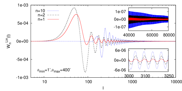
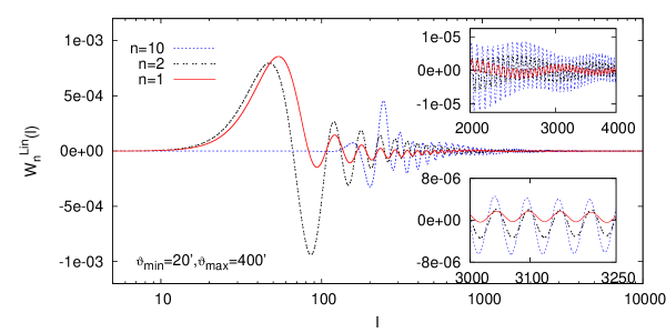
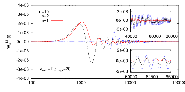
Figure 1: The weight functions $W_{n}^{\mathrm{Lin}}(\ell)$ are the Hankel transforms of $T_{\pm}^{\mathrm{Lin}}(\vartheta)$ as in Eq. $\eqref{Wn}$. In the blow-ups, the two modes of oscillation for each $W_{n}^{\mathrm{Lin}}$ can be seen, the lower frequency mode and the higher frequency mode which are inversely proportional to $\vartheta_{\mathrm{min}}$ and $\vartheta_{\mathrm{max}}$, respectively. The overall amplitude of the oscillations strongly depends on $n$ and $\vartheta_{\mathrm{max}}$.

As is explained in SEK, the Log-COSEBIs are more efficient for a cosmic shear analysis. The reason is that unlike the linear filter functions which oscillate fairly uniformly in linear scale, the logarithmic $T_{+n}^{\mathrm{Log}}$ have their roots fairly uniformly distributed in $\log(\vartheta)$, i.e., they are more sensitive to variations of $\xi_{\pm}$ on smaller scales. Combining this property with the fact that most of the cosmic shear information is contained in these smaller scales shows that it is more reasonable to employ Log-COSEBIs. In the next section we will show the difference of the Log- and Lin-COSEBIs using our figure-of-merit.

In Fig. 1 and Fig. 2 the behavior of linear and logarithmic COSEBIs weight functions, $W_{n}^{\mathrm{Lin}}(\ell)$ and $W_{n}^{\mathrm{Log}}(\ell)$, for three angular ranges can be seen. The $W_{n}^{\mathrm{Log}}(\ell)$ and $W_{n}^{\mathrm{Lin}}(\ell)$ have different yet similar oscillatory properties. They both die out rapidly with increasing $\ell$ but the lower frequency oscillations of $W_{n}^{\mathrm{Log}}(\ell)$ are more prominent. They show approximately the same inverse relation to $\vartheta_{\mathrm{max}}$ and $\vartheta_{\mathrm{min}}$ for their lower and upper limits.

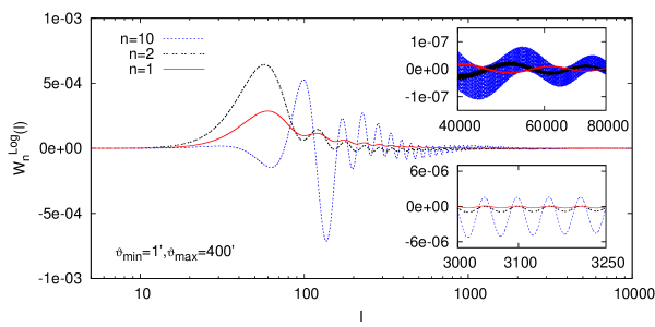
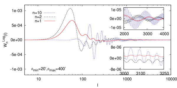
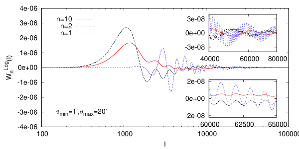
Figure 2: The weight functions $W_{n}^{\mathrm{Log}}(\ell)$ are the Hankel transformation of $T_{\pm}^{\mathrm{Log}}(\vartheta)$ as in Eq. $\eqref{Wn}$. Similar to the $W_{n}^{\mathrm{Lin}}$, the position of the first peak depends mainly on $\vartheta_{\mathrm{max}}$ and is rather insensitive to $\vartheta_{\mathrm{min}}$. The difference between the two sets of linear and logarithmic function can be seen most prominently in the blow-ups; the lower frequency oscillations are more pronounced in this case.

3 Cosmological Model

The cosmological model assumed in the present work is a wCDM model (Peebles & Ratra 2003 and references therein), i.e., a cold dark matter model including a dynamical dark energy with an equation-of-state parameter $w_{0}$. The fiducial value of the parameters involved are listed in Tab. 1.

The starting point in the analysis is to derive the matter power spectrum. For the linear power spectrum we used the Bond & Efstathiou (1984) transfer function, and the halo fit formula of Smith et al. (2003) for a fit of the non-linear regime.

To calculate the convergence power spectrum we need the redshift distribution of galaxies. The overall redshift probability distribution is parametrized by

$$p(z)=\frac{\beta}{z_{0}\>\Gamma[(1+\alpha)/\beta]}\left(\frac{z}{z_{0}}\right)^{\alpha}\exp\left[-\left(\frac{z}{z_{0}}\right)^{\beta}\right]\;,$$ (13)

which represents the galaxy distribution fairly well (it is a generalization of Brainerd et al. 1996). The parameters, $\alpha$, $\beta$, and $z_{0}$ depend on the survey. We consider a medium and a large survey (hereafter MS and LS respectively). The MS has the same area as the CFHTLS (Fu et al. 2008), a current survey, while the LS covers the whole extragalactic sky and represents future surveys. The parameters of our two model surveys are given in Tab. 2, and the corresponding redshift distributions are plotted in Fig. 3.

Table 1: The fiducial cosmological parameters consistent with WMAP 7-years results. The normalization of the power spectrum, $\sigma_{8}$, is the standard deviation of perturbations in a sphere of radius 8 $\>h^{-1}$Mpc today. $\Omega_{\mathrm{m}}$, $\Omega_{\Lambda}$, and $\Omega_{\mathrm{b}}$ are the matter, the dark energy and the baryonic matter density parameters, respectively. $w_{0}$ is the dark energy equation of state parameter, which is equal to the ratio of dark energy pressure to its density. The spectral index, $n_{\mathrm{s}}$, is the slope of the primordial power spectrum. The dimensionless Hubble constant, in $H_{0}=100h$ km s^-1 Mpc^-1, characterizes the rate of expansion today.

$\sigma_{8}$	$\Omega_{\mathrm{m}}$	$\Omega_{\Lambda}$	$w_{0}$	$n_{\mathrm{s}}$	$h$	$\Omega_{\mathrm{b}}$
0.8	0.27	0.73	$-1.0$	0.97	0.70	0.045

Table 2: The redshift distribution parameters and the survey parameters for our medium and large surveys. $\alpha$, $\beta$, and $z_{0}$ determine the total redshift distribution of sources, while $z_{\mathrm{min}}$ and $z_{\mathrm{max}}$ indicate the minimum and the maximum redshifts of the sources considered. $A$ is the survey area in units of deg², $\sigma_{\epsilon}$ is the galaxy intrinsic ellipticity dispersion, and $\bar{n}$ is the mean number density of sources per square arcminute in the field.

	z-distribution parameters					survey parameters
	$\alpha$	$\beta$	$z_{0}$	$z_{\mathrm{min}}$	$z_{\mathrm{max}}$	$A$	$\sigma_{\epsilon}$	$\bar{n}$
MS	0.836	3.425	1.171	0.2	1.5	170	0.42	13.3
LS	2.0	1.5	0.71	0.0	2.0	20000	0.3	35

Constructing the Fisher matrix requires the derivatives of the E-mode COSEBIs and of their covariances with respect to the parameters. For example, to take the derivative with respect to $\Omega_{\mathrm{m}}$, its relation to the shape parameter, $\Gamma$, should be notified. In the present work we use the Sugiyama (1995) relation,

$$\Gamma=\Omega_{\mathrm{m}}\>h\exp[-\Omega_{\mathrm{b}}(1+\sqrt{2h}/\Omega_{\mathrm{m}})]\;.$$ (14)

In their derivatives with respect to $\Omega_{\mathrm{m}}$, SEK assumed a constant $\Gamma$, equivalent to allowing $h$ or $\Omega_{\mathrm{b}}$ to vary accordingly (the only dependence of the convergence power spectrum on $h$ or $\Omega_{\mathrm{b}}$ comes through $\Gamma$). In the present work $h$ and $\Omega_{\mathrm{b}}$ are independent parameters and $\Gamma$ depends explicitly on $\Omega_{\mathrm{m}}$. The difference between the two approaches is not negligible, as shown in Fig. 4 which displays the derivative of the power spectrum with respect to $\Omega_{\mathrm{m}}$ in both cases. This difference is due to the non-linear relation between $h$ and $\Gamma$. To justify our choice of parametrization, we just mention that the constraints from cosmological probes on $h$ is tighter compared to $\Gamma$, and that makes it a more natural choice especially when priors are used.

Figure 3: The overall source redshift probability distribution of source galaxies assumed for the two surveys. LS has a deeper source distribution compared to MS.

Figure 4: The absolute value of the derivative of the convergence power spectrum with respect to $\Omega_{\mathrm{m}}$. Both of the curves rely on a five point stencil method where 4 nearby points have to be evaluated. The solid curve is drawn assuming all parameters are fixed except $\Omega_{\mathrm{m}}$ and $\Gamma$, in contrast to the dotted curve where instead of $\Gamma$, $h$ or $\Omega_{\mathrm{b}}$ are variable.

4 COSEBIs Covariance

Fig. 5 shows the noise-covariance of linear and logarithmic E-mode COSEBIs for the model parameters of the MS (the covariance has a similar behavior in the case of the LS but with a different amplitude). This covariance is calculated from Eq. (2) assuming a single source redshift distribution (Eq. 13). Moreover, by defining the correlation coefficients of COSEBIs,

$$r_{MN}=\frac{C^{\mathrm{E}}_{MN}}{\sqrt{C^{\mathrm{E}}_{MM}C^{\mathrm{E}}_{NN}}}\;,$$ (15)

the behavior of the off-diagonal terms becomes clearer. (The capital subscripts $N$ and $M$ can be different from the COSEBIs subscripts, if several source populations are considered; see below for more details.) Fig. 6 compares the correlation coefficients for three different choices of the angular range, $[1^{\prime},400^{\prime}]$, $[20^{\prime},400^{\prime}]$, and $[1^{\prime},20^{\prime}]\thinspace$, at a fixed $M=9$.

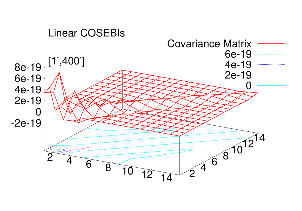
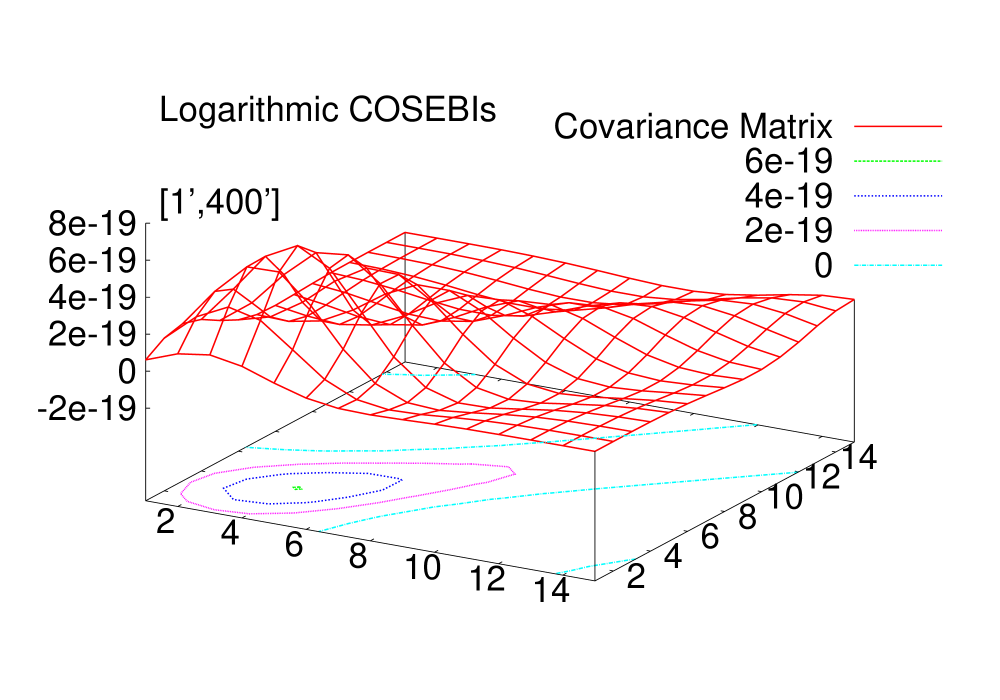
Figure 5: A 3D representation of the non-tomographic covariance of 15 E-mode COSEBIs for an angular range of $[1^{\prime},400^{\prime}]$, for MS parameters. The $x$- and $y$- axes correspond to the elements of the covariance matrix, and the value of the vertical axis shows the value of the covariance of the corresponding element. A contour representation of the covariance is shown for each plot at its base.

Figure 6: The correlation coefficients of non-tomographic COSEBIs for different angular ranges $[\vartheta_{\rm min},\vartheta_{\rm max}]$ at $m=9$, for the MS parameters. Here $M$, the capital subscripts, are equal to the COSEBIs mode, $m$.

Figure 7: A representation of a tomographic covariance. In this diagram 3 redshift-bins (1,2,3) and 5 COSEBIs modes are assumed to be present. The blow-up shows one of the covariance building blocks; the numbers 1-5 show the COSEBIs mode considered, e.g. 15 means the covariance of $E_{1}$ and $E_{5}$. The numbers on the sides of the matrix show which combination of redshift bins is considered, e.g., 12 means the covariance of redshift-bins 1 and 2 is relevant. Due to symmetry, only a part of the covariance elements have to be calculated, here shown in pink.

Figure 8: The correlation coefficients of COSEBIs for an angular range of $[1^{\prime},400^{\prime}]$ and 4 redshift bins. In total, 15 COSEBIs modes are considered for each graph. The $r_{MN}$ is shown for $M=7$ corresponding to $E_{7}^{11}$, and for $M=82$ corresponding to $E_{7}^{23}$.

Figure 9: A comparison between a simplified and complete Fisher analysis, using Log-COSEBIs. The asterisks show the case where the derivatives of the covariance is taken into account (the first part of Eq. 17) while the squares show the simplified case where we assume these derivatives are zero, in calculating $f$. Here $\sigma_{8}$ is the only free parameter, whereas the rest of the parameters is fixed to their fiducial values.

Cosmic shear analysis, as we will see in Sect. 5, provides more information when redshift information is available. In practice the redshifts of galaxies are estimated using several photometric filters (see e.g. Hildebrandt et al. 2010), from which an overall distribution for the source galaxies is obtained. The distribution is then divided into a number of photometric redshift bins. The photometric redshifts are not exact, so the true redshift distributions will overlap. Therefore, instead of redshift bins, in general one has to consider redshift distributions. However, for simplicity, in the present work we have assumed redshift bins with sharp cuts and no overlap. In addition, the bins are selected such that the number of galaxies in each bin is the same.

In general, a tomographic covariance for $r$ redshift bins consists of $[r(r+1)/2]^{2}$ building blocks, each of which is a covariance matrix of $(E^{ij}_{n},E^{kl}_{m})$ where $i,j,k,l$ are fixed and $n,m=1,2,...,n_{\mathrm{max}}$. This means in total the covariance matrix has $[r(r+1)\>n_{\mathrm{max}}]^{2}/4$ elements, where $n_{\mathrm{max}}$ is the maximum number of COSEBIs modes considered.

Nevertheless, a covariance matrix is by definition symmetric and a tomographic covariance is made up of smaller covariances, i.e., only $x(x+1)/2\times n_{\mathrm{max}}(n_{\mathrm{max}}+1)/2$ elements, with $x=r(r+1)/2$, have to be calculated, the rest are equal to these (see Fig. 7).

The covariance of the $E^{ij}_{n}$ depends on six indices; in order to apply normal matrix operations, the three indices of $E^{ij}_{n}$ are combined into one ‘superindex’ $N$, given by

$$N=\Big{[}(i-1)\times r-\frac{(i-1)(i-2)}{2}+(j-i)\Big{]}\times n_{\mathrm{max}}+n\;,$$ (16)

where $r$ is the total number of redshift bins and $n_{\mathrm{max}}$ is the total number of COSEBIs modes.

Using the new labeling, the correlation coefficients of $E^{11}_{7}$ and $E^{23}_{7}$ (corresponding to $N=7$ and $N=82$, respectively) with the other $E^{ij}_{n}$ is shown in Fig. 8, where 15 COSEBIs modes and 4 redshift bins are considered. Each of the peaks in the figure correspond to the correlation coefficient of $E^{11}_{7}$ and $E^{ij}_{7}$. The highest peak with $r=1$ occurs for $M=N$, while the rest of the peaks are correlations between different redshift bins. The Log-COSEBIs show larger noise-correlations between different modes compared to Lin-COSEBIs, which may persuade one to choose the Lin-COSEBIs for cosmic shear analysis. However, the Log-COSEBIs compensate this apparent disadvantage by requiring fewer modes to saturate the Fisher information level for relevant cosmological parameters compared to the linear ones, i.e., the number of covariance elements that have to be calculated for Lin-COSEBIs is higher and hence determining their covariance matrix is more time consuming, especially when redshift binning is considered. Consequently, in Sect. 5 we mainly employ Log-COSEBIs to analyze tomographic Fisher information.

5 Results of Fisher analysis

5.1 Figure-of-merit

In this section we carry out a figure-of-merit analysis to demonstrate the capability of COSEBIs to constrain cosmological parameters from cosmic shear data. Our figure-of-merit, $f$, based on the Fisher matrix, quantifies the credibility of the estimated parameters. In general, for any unbiased estimator, the Fisher matrix gives the lower limit of the errors on parameter estimations (see e.g. Kenney & Keeping 1951 and Kendall & Stuart 1960 for details).

The Fisher matrix is related to the COSEBIs by

$$F_{ij}=\frac{1}{2}\mathrm{Tr}[C^{-1}\>C_{,i}\>C^{-1}\>C_{,j}+C^{-1}\>M_{ij}]\;,$$ (17)

where $C$ is the COSEBIs covariance, $M_{ij}=\boldsymbol{E}_{,i}\;\boldsymbol{E}_{,j}^{\mathrm{T}}+\boldsymbol{E}_{,j}\>\boldsymbol{E}_{,i}^{\mathrm{T}}$, $\boldsymbol{E}$ is the vector of the E-mode COSEBIs, and the commas followed by subscripts indicate partial derivatives with respect to the cosmological parameters (see Tegmark et al. 1997 for example). We define our figure-of-merit, $f$, in a very similar manner to SEK

$$f=\left(\frac{1}{\sqrt{\mathrm{det}\>F}}\right)^{1/n_{\mathrm{p}}}\;,$$ (18)

where $n_{\mathrm{p}}$ is the number of free parameters considered. In the following analysis, we will assume for simplicity that the first term in Eq. $\eqref{FisherTeg}$ is much smaller than the second and can thus be neglected. Note that this approximation becomes more realistic in the case of a large survey area, since the first term on the r.h.s. of Eq. $\eqref{FisherTeg}$ does not depend on the survey area, while the second term is proportional to it (recall that $C\varpropto 1/A$ or in other words $C^{-1}\varpropto A$). We checked that our medium survey is already big enough for this approximation to hold (see Fig. 9).

With the definition $\eqref{f}$ we compress the Fisher matrix into a one-dimensional quantity, which provides a measure of the geometric mean of the standard deviations of the parameters; e.g. in the case of one free parameter $\phi$, $f(\phi)$ is equal to the standard deviation $\sigma(\phi)$ of that parameter.

Figure 10: A comparison between the Log- and Lin-COSEBIs Fisher analysis results for two sets of assumptions, where $\sigma_{8}$ and $\Omega_{\mathrm{m}}$ are the free parameters and the rest is fixed to their fiducial values. In one case the shape parameter $\Gamma$ is held fixed, while in the other it is left as a variable depending on $\Omega_{\mathrm{m}}$ and the fiducial values of $h$ and $\Omega_{\mathrm{b}}$ (according to Eq. 14). The same analysis is also carried out for the Full-COSEBIs and the shear 2PCFs.

Figure 11: These plots show one of our consistency checks. It is a comparison between the Lin- and Log-COSEBIs results for LS with a single (left panel) and two galaxy redshift distributions (right panel), including all of the 7 parameters. Apart from very small numerical inaccuracies, both sets of COSEBIs saturate to the same value, as expected. There are two solid lines in each plot. The line with the higher value shows the value of Log-COSEBIs at $n_{\mathrm{max}}=20$, and the other line shows the value of $f$ as obtained from the shear 2PCFs. The slightly smaller value of $f$ in the latter case (this difference is not visible in the plot) is related to the fact that the analysis from the shear 2PCFs implicitly assume the absence of B-modes, and thus contains information from very large-scale modes which, however, cannot be uniquely assigned to either E- or B-modes. The comparison of the two plots shows that dividing the galaxies into two redshift bins not only increases the information content of the Fisher analysis but also decreases the number of COSEBIs modes needed. Note that the $x$-axis of the single redshift distribution plot starts from 7, the other one from 3.

5.2 Assumptions and parameter settings

For our cosmic shear analysis we considered a medium (MS) and a large survey (LS) as explained in Sect. 3. We have also studied the effect of a Gaussian prior, in the form of a Fisher matrix. This prior is the inverse of the WMAP7 parameter covariance matrix from the final iteration (5000 sample points) of a Population Monte Carlo (PMC) run (see Kilbinger et al. 2010), called the CMB prior from here on. We implement the prior by adding the Fisher matrices of our COSEBIs analysis and the CMB prior. The value of the CMB prior is shown in terms of $f(\phi)$ in the first column of Tab. 3 for each of the parameters.

We consider three different angular ranges, $[1^{\prime},20^{\prime}]\>$, $[1^{\prime},400^{\prime}]\>$, and $[20^{\prime},400^{\prime}]\>$. The motivation for this choice is as follows: We consider a total interval of $[1^{\prime},400^{\prime}]\>$ where the flat sky approximation is still valid up to the maximum separation and galaxy shapes are easily distinguishable for the minimum separation; also, $\vartheta_{\rm min}=1^{\prime}$ avoids the scales where baryonic effects are expected to have the strongest ifluence. We further divide this interval into two non-overlapping parts with $\vartheta_{\rm max}/\vartheta_{\rm min}=20$, to compare cosmic shear information on small and large scales. The small-scale range, $[1^{\prime},20^{\prime}]\>$ may apply for a cosmic shear survey of individual one square degree fields. The large scale interval, $[20^{\prime},400^{\prime}]\>$ could be used for very conservative analyses where non-linear and baryonic effects are to be avoided.

In Sect. 5.3 we show the value of $f$ for two parameters while the rest are fixed to their fiducial values for the MS, and also for all seven parameters for the LS. In principle we could show all of the possible combinations for parameters, nevertheless finding the error on each of the parameters seems a more relevant task. Therefore, the rest of our analysis, carried out in Sect. 5.4, is done for a single parameter, $\phi$, where $f(\phi)=\sigma_{\phi}$.

To find the value of $f$ for a single parameter we use two approaches. In one approach we fix the six other parameters to their fiducial values in Tab. 1, while in the other case we marginalized over the remaining six parameters.

For each setup we investigate the amount of information with respect to the number of COSEBIs modes considered. In addition we analyze the behavior of $f$ with the number of redshift bins considered.

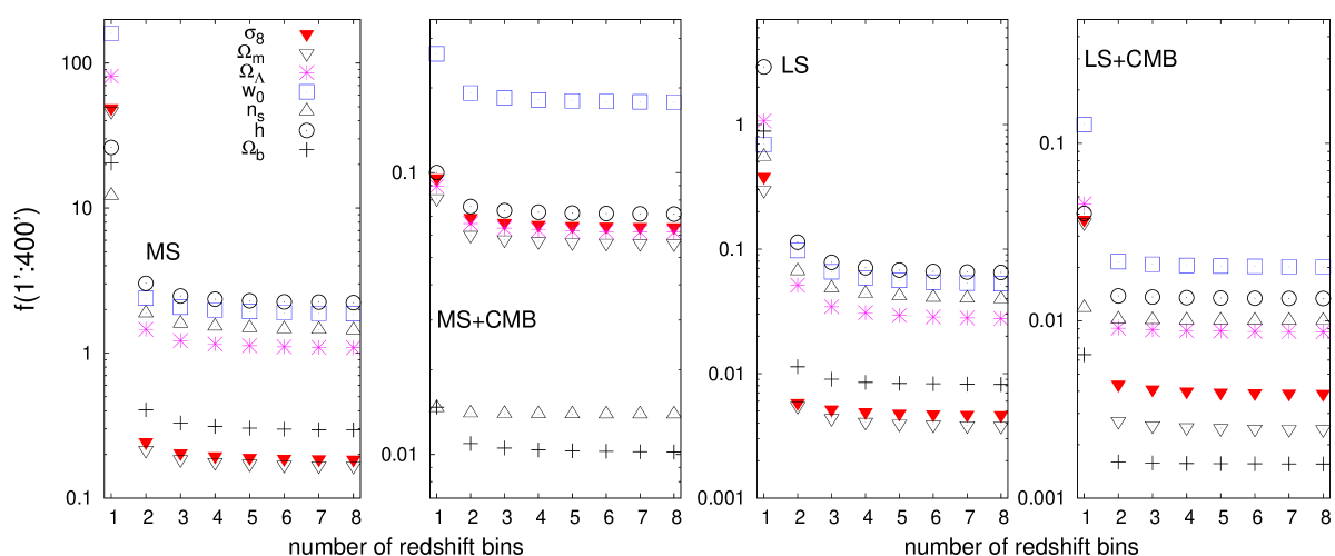
Figure 12: The dependence of the COSEBIs saturated information content in form of $f$ for each of the seven parameters while the rest is marginalized over. The above plots are relevant to MS and LS parameters for an angular ranges of $[1^{\prime},400^{\prime}]\>$. The redshift dependence of $f$ is very outstanding here and hence we needed to use logarithmic scales for the $y$-axes, especially in the cases where cosmic shear analysis is done without any priors.

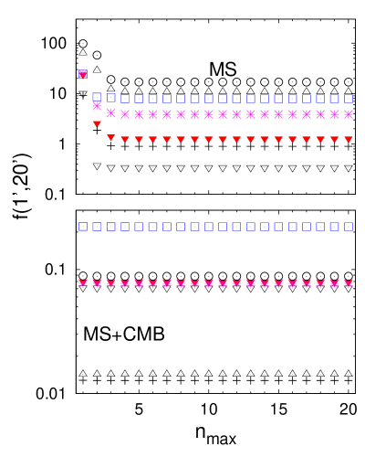
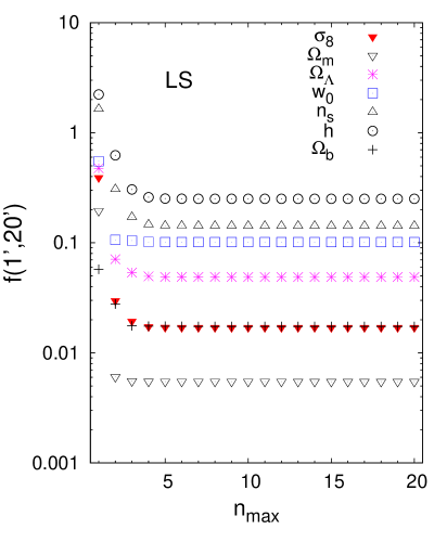
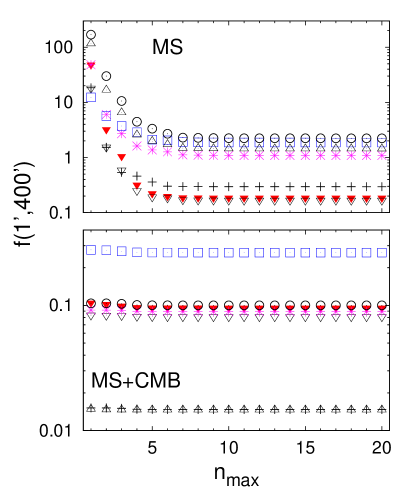
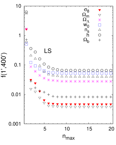
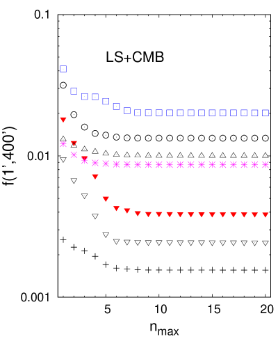
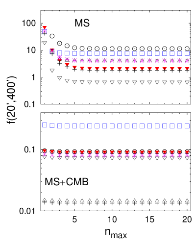
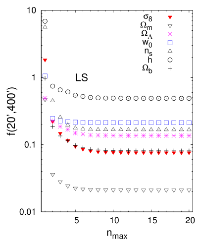
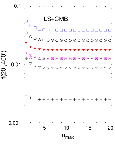
Figure 13: Plots of figure-of-merit values with respect to the number of Log-COSEBIs modes considered for two surveys with the three angular ranges $[1^{\prime},20^{\prime}]\>$, $[1^{\prime},400^{\prime}]\>$, $[20^{\prime},400^{\prime}]\>$. Here all the parameters except one is marginalized over. The first column correspond to MS (top plots) and MS+CMB (bottom plots) and the next two to LS and LS+CMB correspondingly. Eight redshift bins are used here. The CMB prior flattens the curves, especially in the case of MS, where WMAP7 puts tighter constrains on the parameters.

5.3 Properties of COSEBIs

For a fixed number of modes, the Log-COSEBIs are more sensitive than the Lin-COSEBIs to structures of the shear 2PCFs on small scales. Here we show its effect on the Fisher analysis. We investigate the dependence of $f$ on the number $n_{\rm max}$ of COSEBIs modes incorporated in the analysis.

SEK have shown the difference between the behavior of the Lin- and Log-COSEBIs for two parameters, $\sigma_{8}$ and $\Omega_{\mathrm{m}}$, with $\Gamma$ fixed (their definition of $f$ and fiducial values of parameters are slightly different from ours). Similar to their work, we here compare the values of $f$ for the same two parameters with Lin- and Log-COSEBIs. In addition, we inspect the difference between a fixed shape parameter, or its dependence as given in Eq. $\eqref{shapeparameter}$.

Fig. 10 is a representation of our inspection for the MS in the angular range of $[1^{\prime},400^{\prime}]\>$. Two general conclusions come out of this comparison: (1) $f$ for fixed and dependent $\Gamma$ converges to the same value for the Lin- and Log-COSEBIs. (2) The values of $f$ for a fixed or dependent $\Gamma$ are different, and also the convergence rate is different. E.g., the Lin-COSEBIs reach the saturated $f$ value for $n_{\rm max}\approx 40$ for a variable $\Gamma$, while in the other case, only 25 modes are needed. This effect is less dramatic in the case of Log-COSEBIs (they need 7 modes for a variable $\Gamma$ and 5 modes for a constant one), since they generally converge faster. Similarly in Fig. 11, we visualize our consistency check by showing that the values of $f$ for Log- and Lin-COSEBIs converge to the same value for seven parameters.

In Figs. 10 and 11, we also show the value of $f$ as derived directly from the shear 2PCFs, i.e., without E-/B-mode separation. As expected, in this case $f$ becomes slightly smaller since it is now implicitly assumed that all the signal is due to E-modes. However, this is not justified in general; for example, very large-scale modes (i.e., small $\ell$) enter $\xi_{+}(\vartheta)$ even for small $\vartheta$, and such modes cannot be uniquely assigned to either E- or B-modes. Thus, the decrease of $f$, and accordingly, the information gain is just an apparent one, bought by making a strong assumption. The relative difference between the 2PCFs and the converged Lin-/Log-COSEBIs values for $f$ is larger for the variable $\Gamma$ case, since here small-$\ell$ modes, which are filtered out in the COSEBIs, contain information about the power spectrum shape.

We also considered as further possibility that the requirement of finite support for the $\xi_{-}(\vartheta)$ is dropped, and call this ‘Full-COSEBIs’. They form a complete set of functions on $[\vartheta_{\rm min},\vartheta_{\rm max}]$, without the constraints given in Eq. $\eqref{T+cond}$. Though not physically reasonable, the Full-COSEBIs are equivalent to measuring $\xi_{+}$ only, on the same interval. As can be seen from Fig. 10, the full COSEBIs yield a slightly lower value of $f$ than the true COSEBIs, showing that $\xi_{-}$ on scales larger than $\vartheta_{\rm max}$ adds apparent information, which, however, is not observable. We stress here that the E-/B-mode correlation functions $\xi_{\rm E/B}$, introduced by Crittenden et al. (2002) and Schneider et al. (2002a), are essentially equivalent to the Full-COSEBIs, since they are also based on the assumption that $\xi_{-}$ can be measured to arbitrarily large separations – which, however, is not possible. Therefore, a cosmic shear analysis based on $\xi_{\rm E}$ (e.g., Fu et al. 2008; Lin et al. 2011) underestimates the uncertainties of cosmological parameters.

Furthermore, we compare the Lin- and Log-COSEBIs for LS parameters in Fig. 11, for one and two redshift bins. The $x$-axis in the left plot starts from 7 in contrast to the right one which starts from 3. The reason is that to constrain $n_{\mathrm{p}}$ parameters at least $n_{\mathrm{p}}$ equations are needed, i.e., if one redshift bin is considered, $n_{\mathrm{p}}$ COSEBIs modes should be accounted for to produce a covariance matrix with at least $n_{\mathrm{p}}$ $\times$ $n_{\mathrm{p}}$ elements. For more than one redshift bin, a smaller number of COSEBIs modes are sufficient, subsequently the saturation rate of $f$ is faster, as is visible in the right plot in the figure. Recall that 2 redshift bins means 3 different redshift combinations, i.e., for 7 parameters, the smallest integer not less than $\lceil 7/3\rceil=3$ COSEBIs modes are needed.

5.4 Forecast for parameter constraints

This section is dedicated to our final results according to the assumptions and parameters explained in Sect. 5.2.

Fig. 12 shows the dependence of $f$ for 20 Log-COSEBIs modes and for the $[1^{\prime},400^{\prime}]$ angular range on the number of galaxy distributions (i.e., redshift bins), where all but one parameter are marginalized over. Dividing the galaxy distribution into more than 4 redshift bins does not change the value of $f$ considerably. Nevertheless, a much larger number of redshift bins is required to control and correct for systematic effects, e.g., coming from intrinsic alignments (see for example Joachimi & Schneider 2010 and references therein).

We also show the dependence of $f$ on $n_{\rm max}$, for 8 redshift bins and marginalized parameters, in Fig. 13. Comparing the cosmic shear analysis with and without CMB prior, we see from the figure that the prior in general flattens the curves. However, the curves are flatter for MS+CMB than LS+CMB as a result of the larger difference between the LS and the CMB prior.

The constraints on each of the cosmological parameters behave differently with respect to the number of COSEBIs modes or redshift bins considered. For marginalized parameters where the behavior of parameters is entangled, their curves show a similar decline.

By comparing the different angular ranges we conclude that a wider angular range needs more modes to extract all information. We also note that the behavior of the seven parameters are not similar and each of them should be followed separately.

Based on the results from these two figures, we will report additional results for $n_{\rm max}=20$, where the value of $f$ is converged, and for either one or eight redshift bins. These results are shown in Tab. 3 in the form of $f(\phi)$ for different cases. We have compared these values with Debono et al. (2010), and found them fully consistent.

In the following we explain our conclusions from the two mentioned figures and Tab. 3 in more detail:

Table 3: Listed below are the values of $f$ for 20 Log-COSEBIs modes, where the saturation level is well reached for all the cases. The first column indicates which parameter is free, the rest of the parameters are either fixed (4th-7th columns) or marginalized over (8th-11th columns). The two numbers written in the first-column box of each parameter in parenthesis are the corresponding $f$ values from CMB alone, for fixed and marginalized parameters, respectively. The second and third columns show the survey and angular range considered. The values of $f$ for one and eight redshift bins are presented here for comparison. MS and LS stand for a medium and large survey, respectively.

			Fixed parameters				Marginalized parameters
			without Prior		+ CMB		without Prior		+ CMB
			1 z-bin	8 z-bins	1 z-bin	8 z-bins	1 z-bin	8 z-bins	1 z-bin	8 z-bins
$\Omega_{\mathrm{b}}$	MS	$[1^{\prime},20^{\prime}]$	3.61E$-$2	3.30E$-$2	9.39E$-$4	9.39E$-$4	2.79E$+$2	8.95E$-$1	1.52E$-$2	1.27E$-$2
(9.39E$-$4)		$[1^{\prime},400^{\prime}]$	3.28E$-$2	2.83E$-$2	9.39E$-$4	9.39E$-$4	2.04E$+$1	2.95E$-$1	1.47E$-$2	1.02E$-$2
		$[20^{\prime},400^{\prime}]$	1.07E$-$1	6.88E$-$2	9.39E$-$4	9.39E$-$4	1.26E$+$2	1.79E$+$0	1.51E$-$2	1.34E$-$2
(1.52E$-$2)	LS	$[1^{\prime},20^{\prime}]$	7.39E$-$4	6.80E$-$4	5.81E$-$4	5.51E$-$4	4.65E+0	1.74E$-$2	8.67E$-$3	1.64E$-$3
		$[1^{\prime},400^{\prime}]$	7.15E$-$4	6.41E$-$4	5.69E$-$4	5.29E$-$4	8.86E$-$1	8.19E$-$3	6.44E$-$3	1.56E$-$3
		$[20^{\prime},400^{\prime}]$	7.07E$-$3	3.31E$-$3	9.31E$-$4	9.04E$-$4	5.01E+0	8.11E$-$2	1.35E$-$2	2.51E$-$3
$h$	MS	$[1^{\prime},20^{\prime}]$	1.32E$-$1	1.19E$-$1	2.09E$-$2	2.08E$-$2	3.38E+2	1.69E+1	1.04E$-$1	8.81E$-$2
(2.11E$-$2)		$[1^{\prime},400^{\prime}]$	1.21E$-$1	1.06E$-$1	2.08E$-$2	2.07E$-$2	2.61E+1	2.23E+0	1.00E$-$1	7.13E$-$2
		$[20^{\prime},400^{\prime}]$	3.91E$-$1	2.78E$-$1	2.11E$-$2	2.11E$-$2	1.11E+3	1.13E+1	1.03E$-$1	9.26E$-$2
(1.04E$-$1)	LS	$[1^{\prime},20^{\prime}]$	2.73E$-$3	2.52E$-$3	2.71E$-$3	2.50E$-$3	1.70E+1	2.51E$-$1	5.18E$-$2	1.46E$-$2
		$[1^{\prime},400^{\prime}]$	2.65E$-$3	2.40E$-$3	2.63E$-$3	2.38E$-$3	2.91E+0	6.49E$-$2	4.02E$-$2	1.33E$-$2
		$[20^{\prime},400^{\prime}]$	2.67E$-$2	1.37E$-$2	1.66E$-$2	1.15E$-$2	1.81E+1	4.89E$-$1	9.80E$-$2	2.57E$-$2
$n_{\mathrm{s}}$	MS	$[1^{\prime},20^{\prime}]$	1.07E$-$1	9.80E$-$2	7.81E$-$3	7.81E$-$3	7.53E+2	1.08E+1	1.47E$-$2	1.43E$-$2
(7.83E$-$3)		$[1^{\prime},400^{\prime}]$	9.08E$-$2	7.87E$-$2	7.80E$-$3	7.79E$-$3	1.22E$+$1	1.44E$+$0	1.46E$-$2	1.39E$-$2
		$[20^{\prime},400^{\prime}]$	1.95E$-$1	1.54E$-$1	7.83E$-$3	7.82E$-$3	1.04E$+$2	3.97E$+$0	1.50E$-$2	1.45E$-$2
(1.58E$-$2)	LS	$[1^{\prime},20^{\prime}]$	2.12E$-$3	1.98E$-$3	2.05E$-$3	1.92E$-$3	8.47E$+$0	1.42E$-$1	1.28E$-$2	1.05E$-$2
		$[1^{\prime},400^{\prime}]$	2.03E$-$3	1.83E$-$3	1.96E$-$3	1.79E$-$3	5.52E$-$1	3.96E$-$2	1.18E$-$2	1.00E$-$2
		$[20^{\prime},400^{\prime}]$	1.29E$-$2	8.15E$-$3	6.70E$-$3	5.65E$-$3	4.11E$+$0	1.67E$-$1	1.30E$-$2	1.24E$-$2
$w_{0}$	MS	$[1^{\prime},20^{\prime}]$	1.40E$-$1	1.18E$-$1	3.64E$-$2	3.59E$-$2	2.70E$+$2	7.89E$+$0	2.70E$-$1	2.21E$-$1
(3.77E$-$2)		$[1^{\prime},400^{\prime}]$	1.02E$-$1	8.69E$-$2	3.54E$-$2	3.46E$-$2	1.60E$+$2	1.87E$+$0	2.64E$-$1	1.78E$-$1
		$[20^{\prime},400^{\prime}]$	3.55E$-$1	3.06E$-$1	3.75E$-$2	3.74E$-$2	4.11E$+$2	7.55E$+$0	2.80E$-$1	2.43E$-$1
(2.83E$-$1)	LS	$[1^{\prime},20^{\prime}]$	3.04E$-$3	2.72E$-$3	3.03E$-$3	2.71E$-$3	3.59E+1	1.01E$-$1	1.68E$-$1	2.65E$-$2
		$[1^{\prime},400^{\prime}]$	2.83E$-$3	2.49E$-$3	2.82E$-$3	2.48E$-$3	6.93E$-$1	5.26E$-$2	1.28E$-$1	2.01E$-$2
		$[20^{\prime},400^{\prime}]$	2.12E$-$2	1.73E$-$2	1.85E$-$2	1.57E$-$2	3.75E+1	2.12E$-$1	2.44E$-$1	3.87E$-$2
$\Omega_{\Lambda}$	MS	$[1^{\prime},20^{\prime}]$	1.73E$-$1	1.26E$-$1	1.18E$-$2	1.18E$-$2	3.04E+2	3.86E+0	9.23E$-$2	7.72E$-$2
(1.18E$-$2)		$[1^{\prime},400^{\prime}]$	9.56E$-$2	7.37E$-$2	1.17E$-$2	1.17E$-$2	8.11E+1	1.09E+0	8.94E$-$2	6.15E$-$2
		$[20^{\prime},400^{\prime}]$	2.41E$-$1	1.98E$-$1	1.18E$-$2	1.18E$-$2	1.38E+3	4.04E+0	9.12E$-$2	8.09E$-$2
(9.26E$-$2)	LS	$[1^{\prime},20^{\prime}]$	3.47E$-$3	2.70E$-$3	3.33E$-$3	2.63E$-$3	1.50E+1	4.89E$-$2	5.86E$-$2	9.20E$-$3
		$[1^{\prime},400^{\prime}]$	2.99E$-$3	2.28E$-$3	2.90E$-$3	2.23E$-$3	1.07E+0	2.77E$-$2	4.55E$-$2	8.67E$-$3
		$[20^{\prime},400^{\prime}]$	1.34E$-$2	1.02E$-$2	8.85E$-$3	7.70E$-$3	1.86E+1	1.36E$-$1	8.18E$-$2	1.27E$-$2
$\Omega_{\mathrm{m}}$	MS	$[1^{\prime},20^{\prime}]$	9.32E$-$3	8.26E$-$3	4.06E$-$3	3.96E$-$3	9.27E+1	3.40E$-$1	8.44E$-$2	7.09E$-$2
(4.52E$-$3)		$[1^{\prime},400^{\prime}]$	7.13E$-$3	6.47E$-$3	3.81E$-$3	3.70E$-$3	4.67E+1	1.67E$-$1	8.11E$-$2	5.61E$-$2
		$[20^{\prime},400^{\prime}]$	3.45E$-$2	3.23E$-$2	4.48E$-$3	4.47E$-$3	3.40E+2	6.67E$-$1	8.28E$-$2	7.39E$-$2
(8.56E$-$2)	LS	$[1^{\prime},20^{\prime}]$	2.18E$-$4	2.03E$-$4	2.18E$-$4	2.02E$-$4	9.15E+0	5.48E$-$3	4.83E$-$2	3.05E$-$3
		$[1^{\prime},400^{\prime}]$	2.06E$-$4	1.90E$-$4	2.06E$-$4	1.90E$-$4	2.98E$-$1	3.81E$-$3	3.58E$-$2	2.44E$-$3
		$[20^{\prime},400^{\prime}]$	2.20E$-$3	1.96E$-$3	1.98E$-$3	1.79E$-$3	3.81E+0	2.12E$-$2	7.50E$-$2	8.89E$-$3
$\sigma_{8}$	MS	$[1^{\prime},20^{\prime}]$	1.75E$-$2	1.51E$-$2	1.12E$-$2	1.05E$-$2	1.01E+2	1.27E+0	9.79E$-$2	7.91E$-$2
(1.46E$-$2)		$[1^{\prime},400^{\prime}]$	1.35E$-$2	1.20E$-$2	9.90E$-$3	9.27E$-$3	4.90E+1	1.85E$-$1	9.57E$-$2	6.42E$-$2
		$[20^{\prime},400^{\prime}]$	6.97E$-$2	6.33E$-$2	1.43E$-$2	1.42E$-$2	3.41E+2	2.14E+0	1.07E$-$1	9.23E$-$2
(1.11E$-$1)	LS	$[1^{\prime},20^{\prime}]$	4.05E$-$4	3.65E$-$4	4.04E$-$4	3.65E$-$4	1.01E+1	1.70E$-$2	5.12E$-$2	5.35E$-$3
		$[1^{\prime},400^{\prime}]$	3.82E$-$4	3.43E$-$4	3.82E$-$4	3.43E$-$4	3.82E$-$1	4.66E$-$3	3.73E$-$2	3.88E$-$3
		$[20^{\prime},400^{\prime}]$	4.34E$-$3	3.58E$-$3	4.16E$-$3	3.48E$-$3	4.50E+0	7.61E$-$2	8.99E$-$2	1.78E$-$2

• MS vs. LS vs. CMB prior: In general, because of its much larger survey area and larger galaxy number density, LS puts tighter constraints on all of the parameters than the MS. Furthermore, since the LS is deeper than the MS, it allows more sensitive constraints on parameters which are sensitive to the growth of structure, in particular $w_{0}$. As can be seen from Fig. 13, the requested number of COSEBIs for saturation is slightly higher for the LS since this survey contains more information, but smaller than 20 in all cases.

  The MS constraints on parameters are weaker than the CMB alone for almost all cases. $\Omega_{\mathrm{m}}$ and $\sigma_{8}$, the two parameters for which present cosmic shear studies provide the most relevant constraints, are the only two for which the MS constraints are comparable with CMB. As for the rest of the parameters, except for $f(w_{0},[1^{\prime},400^{\prime}])$ for the case of fixed parameters, the parameter uncertainty of the CMB prior is about one order of magnitude or more smaller than that of the MS. We conclude that the MS is not large enough to be competitive with the CMB for constraining a seven parameter cosmological model. However, the combination of the two slightly tightens the constraints.

  In contrast to the MS, the LS yields parameter constraints which can be considerably stronger than the CMB alone, in particular when tomography is employed. To wit, for the total angular range of $[1^{\prime},400^{\prime}]$ and 8 $z$-bins, the LS errors are smaller than those from the CMB, except for $n_{\mathrm{s}}$ with marginalized parameters. For fixed parameters, the $f$ value resulting from the combination of the LS and the CMB prior is very close to the LS value, whereas it can be much smaller than that of the CMB alone. I.e., we conclude that the resulting constraints from the LS are not dominated by the assumed prior.

  In contrast to the MS, the LS is able to put useful constraints on the parameters, even without tomography and for marginalized parameters. This is seen in the difference between the error values obtained from CMB alone and LS+CMB.

  The relative value of errors on parameters is different between the two surveys. The reason is that the redshift distributions of the two surveys are different (see Tab. 2 and Fig. 3) as seen in the figures. Using redshift information in general is equivalent to using structure evolution information. The large-scale evolution is more visible in the case of a wider redshift distribution which starts from $z=0$, where these structures are more evolved.

• Fixed vs. Marginalized: The difference between the value of $f$ for fixed and marginalized parameters is immense, especially when prior information is not available. However, we can state that, for all cases without priors, $\Omega_{\mathrm{m}}$ is the best constrained parameter. The relative value of the parameters is also different between fixed and marginalized cases. Also for the fixed parameter case, the convergence rate of LS is slower compared to the MS and its relative information content is higher, as expected.

  In contrast to the fixed parameters case, tomography substantially lowers the errors for marginalized parameters.

• Angular ranges: From the table, we find the following common trends for fixed parameters:

  $$f(1^{\prime},400^{\prime})<f(1^{\prime},20^{\prime})<f(20^{\prime},400^{\prime})\;,$$ (19)

  $$\left(\frac{f(1^{\prime},20^{\prime})}{f(1^{\prime},400^{\prime})}\right)_{\mathrm{MS}}>\left(\frac{f(1^{\prime},20^{\prime})}{f(1^{\prime},400^{\prime})}\right)_{\mathrm{LS}}\;,$$ (20)

  $$\left(\frac{f(20^{\prime},400^{\prime})}{f(1^{\prime},400^{\prime})}\right)_{\mathrm{MS}}<\left(\frac{f(20^{\prime},400^{\prime})}{f(1^{\prime},400^{\prime})}\right)_{\mathrm{LS}}\;.$$ (21)

  The first relation shows that there is more information at smaller scales than in the large-scale angular interval, although there is some independent information at larger scales. More interesting are the second and third relations which show that there is more information at smaller scales regarding LS compared to MS, which is a consequence of their different redshift distributions and cuts (see Fig. 3 and Tab. 2). The relations between the $f(\vartheta_{\mathrm{min}},\vartheta_{\mathrm{max}})$ for different angular ranges change when parameters are marginalized over. In this case the above inequalities are no longer valid for all of the parameters.

Fig. 14 shows constraints for two pairs of parameters. In the bottom plot the direction of the contours for the MS are determined by the CMB prior. In this case tomography slightly improves the constraints on both parameters. The top plot, on the other hand, shows the constraints on dark energy parameters. In this case tomographic improvements are more visible. Also here the direction of the contours are different for the two cases.

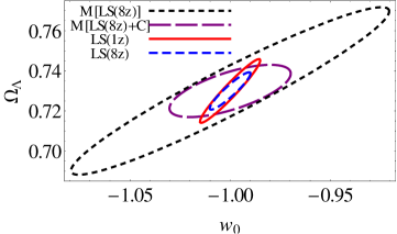
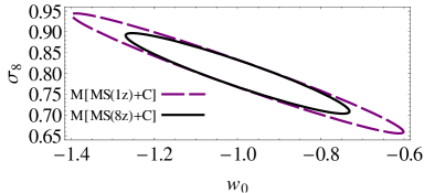
Figure 14: Contour plots of 1$\sigma$ constraints for pairs of parameters. The plot legends are abbreviated to save space. M stands for Marginalized, C for the CMB prior, and #z for the number of redshift bins. Top plot: The 1$\sigma$ contours of $w_{0}$ and $\Omega_{\Lambda}$ for the LS. The two smaller contours are for the case where the five other parameters are held fixed to their fiducial values. Bottom plot: The 1$\sigma$ contours of $\sigma_{8}$ and $w_{0}$ for the MS.

6 Summary and Conclusion

We have generalized the cosmic shear analysis with COSEBIs to include seven cosmological parameters, and investigated the effect of tomography on parameter constraints. For our analysis we mainly used the Log-COSEBIs, although for consistency checks we have shown that Lin-COSEBIs results agree with their logarithmic counterparts. In App. A we show that there are analytic solutions for linear $W_{n}$ functions, which are in principle less computationally demanding.

Besides the number of parameters and the use of redshift information, the main difference to SEK is a technical one: we calculated the COSEBIs and their covariance directly from the power spectrum, without using the 2PCFs as intermediate step. This choice is more convenient for theoretical considerations and highly speeds up the calculations of the COSEBIs covariances, an advantage in particular for the case of tomography. We also confirmed that our method can reproduce the results of SEK.

We investigated the effect of a Gaussian prior on two mock surveys, using three angular ranges on which the shear 2PCFs are asumed to be measured, by Fisher analysis methods. We considered the case that all but one parameter are fixed, as well as that where we marginalize over the other six parameters, in order to find the constraints on a single parameter. The prior was the Fisher matrix resulting from a Population Monte Carlo (PMC) analysis of WMAP7 results. We considered a medium and a large mock survey resembling the state-of-the-art in cosmic shear and that of future all-(extragalactic) sky surveys.

Most importantly, we found that a relatively small number of COSEBIs captures essentially all cosmological information from a cosmic shear survey. Whereas this number is larger than in SEK, due to the higher-dimensional parameter space and the tomographic analysis, COSEBIs not only act as a clean E-/B-mode separating shear statistics, but also as a highly efficient data compression method. We stress that this feature is extremely useful also for evaluating covariances from numerical simulations.

The required number of COSEBIs to saturate the cosmological information is considerably smaller for Log-COSEBIs than for Lin-COSEBIs, which implies a clear preference for the former. It also increases with the number of free parameters, and depends on the parameters considered, the survey, and the angular range on which the 2PCFs are measured. In all cases we considered, fewer than 20 Log-COSEBIs modes were sufficient to reach information saturation. Aside from the tighter constraints of the large survey (LS) on all of the parameters compared to the medium-sized survey (MS), the order of the parameters with respect to their Fisher information is different between the two surveys. Moreover, in general LS requires more COSEBIs modes due to its higher information level. The comparison of the three angular ranges shows that most of the information in cosmic shear is contained at smaller scales which is why the Log-COSEBIs with their finer oscillations towards smaller scales are more sensitive and reach the saturated level of information with fewer modes. However, there is interesting independent information at larger scales, resulting in tighter constraints when using both angular ranges.

We have investigated the dependence of our figure of merit, $f$, on the number of redshift bins considered. In agreement with earlier work, we found that tomography greatly tightens parameter constraints, but the cosmological information saturates at around three or four redshift bins. This, however, does not imply that coarse redshift information is sufficient for future lensing surveys, since good redshift information is required to eliminate systematics from the data, such as intrinsic alignment effects (e.g., King & Schneider 2003 ; Joachimi & Schneider 2008; Joachimi & Bridle 2010)

For future work it will be interesting to investigate the effects of nulling with COSEBIs. Nulling techniques (Joachimi & Schneider 2008) eliminate the intrinsic-intrinsic and intrinsic-shear correlations from observed ellipticity correlations. The intrinsic-intrinsic correlation can be handled by accurate redshift information to eliminate pairs with physical connections. Consequently, one can investigate how the cosmic shear information evolves by doing so, and how many redshift bins are needed in this case. Furthermore, our assumption of a Gaussian covariance becomes unrealistic at small angular scales; hence, it will be interesting to carry out a similar analysis based on more realistic covariances, either obtained from ray-tracing through cosmological density fields or using (semi-)analytic models, such as based on log-normal fields (see Hilbert et al. 2011).

Appendix A Analytic solutions to linear COSEBIs weight functions

Calculating the $W_{n}$ functions and evaluating integrals involving them requires careful methods, as a result of their very oscillating nature. In this section we first show our semi-analytical solutions to $W_{n}^{\mathrm{Lin}}(\ell)$ and at the end discuss our method of integration in more detail.

The filters, $T_{+n}^{\mathrm{Lin}}$, were calculated in SEK. By a simple variable change of $y=\ell\vartheta$, Eq. $\eqref{Wn}$ becomes

$$W_{n}^{\mathrm{Lin}}(\ell)=\frac{1}{\ell^{2}}\int_{\ell\vartheta_{\mathrm{min}}}^{\ell\vartheta_{\mathrm{max}}}\mathrm{d}y\>y\>T_{+n}(y/\ell)\mathrm{J}_{0}(y)\;.$$ (22)

One can write $T_{+n}$ in the form

$$T_{+n}(\vartheta)=\sum_{i=0}^{n+1}a_{ni}\vartheta^{i}\;,$$ (23)

and then rewrite $W_{n}^{\mathrm{Lin}}$ as:

$$W_{n}^{\mathrm{Lin}}(\ell)=\sum_{i=0}^{n+1}\frac{a_{ni}}{\ell^{2+i}}\int_{\ell\vartheta_{\mathrm{min}}}^{\ell\vartheta_{\mathrm{max}}}\mathrm{d}y\>y^{i+1}\mathrm{J}_{0}(x)\;.$$ (24)

We define the functions $S_{n}$ as

$$S_{n}(b):=\int_{0}^{b}\mathrm{d}x\>y^{n+1}\mathrm{J}_{0}(y)\;.$$ (25)

Inserting the above equation into Eq. $\eqref{WnFromSn}$ gives

$$W_{n}^{\mathrm{Lin}}(\ell)=\sum_{i=0}^{n+1}\frac{a_{ni}}{\ell^{2+i}}[S_{i}(\ell\vartheta_{\mathrm{max}})-S_{i}(\ell\vartheta_{\mathrm{min}})]\;.$$ (26)

The $S_{n}$ functions can be obtained using standard Bessel functions relations, which in our case specialize to

$$\frac{\mathrm{d}}{\mathrm{d}y}[y\>\mathrm{J}_{1}(y)]=y\>\mathrm{J}_{0}(y)\;,$$ (27)

$$\mathrm{J}_{-1}(y)-\mathrm{J}_{1}(y)=2\mathrm{J}^{\prime}_{0}(y)\;,$$

$$\mathrm{J}_{-1}(y)=-\mathrm{J}_{1}(y)\;,$$ (28)

$$-\mathrm{J}_{1}(y)=\mathrm{J}^{\prime}_{0}(y)\;,$$ (29)

where the last equation results from the two equations before it.

Using Eqs. $\eqref{J1}$ and $\eqref{J2}$, the following calculations for $S_{n}$ are carried out,

$$S_{n}(b) =\int_{0}^{b}\mathrm{d}y\>y^{n+1}\mathrm{J}_{0}(y)$$

$$=y^{n+1}\mathrm{J}_{1}(y)\Bigr{\rvert}_{0}^{b}-n\int_{0}^{b}\mathrm{d}x\>y^{n}\>\mathrm{J}_{1}(y)$$

$$=y^{n+1}\mathrm{J}_{1}(y)\Bigr{\rvert}_{0}^{b}+n\>y^{n}\mathrm{J}_{0}(y)\Bigr{\rvert}_{0}^{b}-n^{2}\int_{0}^{b}\mathrm{d}y\>y^{n-1}\mathrm{J}_{0}(y)\;,$$ (30)

where we have carried out integration by parts twice. Note that the last term in the above equations is equal to $S_{n-2}$. Consequently, the recursive formula for $S_{n}$ is

$$S_{n}(b)=b^{n+1}\mathrm{J}_{1}(b)+n\>b^{n}\mathrm{J}_{0}(b)-n^{2}\>S_{n-2}(b)\;.$$ (31)

The first two of these functions are

$$S_{0}(b) =\int_{0}^{b}\mathrm{d}y\>y\>\mathrm{J}_{0}(y)=b\>\mathrm{J}_{1}(b)\;,$$ (32)

$$S_{-1}(b) =\int_{0}^{b}\mathrm{d}y\>\mathrm{J}_{0}(y)=b\;_{1}F_{2}[{1/2},{1,3/2},-b^{2}/4]\;,$$ (33)

where ${}_{1}F_{2}$ is the Hypergeometric functions (see Arfken & Weber 1995). Although there is an analytic formula for $S_{-1}$, it is more convenient to solve it numerically using a similar step-wise integration method as was explained in Sect. 2.1 . The only difference here is that the steps are taken between zeros of the Bessel function. A plot of $S_{-1}$ can be seen in Fig. 15.

Figure 15: The weight functions $W_{n}(\ell)$ depend on $S_{n}$ integrals, which are recursively related to each other. Here the shape of the starting function $S_{-1}$ is shown. As is expected it reaches zero as the argument gets smaller and has a highly oscillating behavior similar to its integrand, $\mathrm{J}_{0}$.

The recursive formula in Eq. $\eqref{Snrec}$ can be rewritten as a closed form formula of the form:

$$S_{n}(b) =\mathrm{J}_{1}(b)[b^{n+1}+\sum_{k=1}^{N}(-1)^{k}\prod_{i=0}^{k-1}(n-2i)^{2}b^{n+1-2k}]$$

$$+\mathrm{J}_{0}(b)[nb^{n}+\sum_{k=1}^{N}(-1)^{k}\prod_{i=0}^{k-1}(n-2i)^{2}(n-2k)b^{n-2k}]$$

$$+(-1)^{N+1}\prod_{i=0}^{N}(n-2i)^{2}S_{n-2(N+1)}(b)\;,$$ (34)

where $N$ is

$$N=\left\{\begin{aligned} &\frac{n-2}{2}\qquad n\;\;\mathrm{even}\\ &\frac{n-1}{2}\qquad n\;\;\mathrm{odd}\;.\end{aligned}\right.$$ (35)

To calculate the $T_{+n}^{\mathrm{Lin}}(\vartheta)$ SEK rescaled the angular separation intervals from $[\vartheta_{\mathrm{min}},\vartheta_{\mathrm{max}}]$ to $[-1,1]$ with a variable transformation of the form

$$x=\frac{2(\vartheta-\bar{\vartheta})}{\Delta\vartheta}\;,$$ (36)

with $\bar{\vartheta}=(\vartheta_{\mathrm{min}}+\vartheta_{\mathrm{max}})/2$, $\Delta\vartheta=\vartheta_{\mathrm{min}}-\vartheta_{\mathrm{max}}$ and calculated the results for $t_{+n}^{\mathrm{Lin}}(x)=T_{+n}^{\mathrm{Lin}}(\vartheta)$. The explicit mathematical form of $t_{+1}^{\mathrm{Lin}}(x)$ and $t_{+2}^{\mathrm{Lin}}(x)$ are shown in SEK. One can find the $a_{ni}$ coefficients in Eq. $\eqref{Tcoefs}$ by a change of variable from $x$ to $\vartheta$.

The rest of the $t_{+n}^{\mathrm{Lin}}(x)$ filters are

$$t_{+n}^{\mathrm{Lin}}(x)=\sqrt{\frac{2n+3}{2}}\;P_{n+1}(x)\;,$$ (37)

where $P_{n+1}(x)$ is the Legendre polynomials of order $n+1$. We rewrite the recursive relation for Legendre polynomials using Eq. $\eqref{xtheta}$

$$P_{0}(x) =1\;,$$

$$P_{1}(x) =\frac{2\vartheta}{\Delta\vartheta}-\frac{1}{B}\;,$$

$$P_{n}(x) =\frac{2n-1}{n}\frac{2\vartheta}{\Delta\vartheta}\>P_{n-1}(x)-\frac{2n-1}{n}\frac{1}{B}\>P_{n-1}(x)$$

$$-\frac{n-1}{n}\>P_{n-2}(x)\;,$$ (38)

where $B=\Delta\vartheta/(2\bar{\vartheta})=(\vartheta_{\mathrm{min}}-\vartheta_{\mathrm{max}})/(\vartheta_{\mathrm{min}}+\vartheta_{\mathrm{max}})$ is the relative interval width. Note that the first term in the recursive relation has the highest polynomial order, and the rest have lower order, respectively. We write the Legendre polynomials as polynomials in $\vartheta$

$$P_{n}(x)=\sum_{i=0}^{n}C_{ni}\>\vartheta^{i}\;,$$ (39)

with $C_{ni}$ coefficients

$$C_{00} =1\;,$$

$$C_{11} =\frac{2}{\Delta\vartheta}\;,$$

$$C_{10} =-\frac{1}{B}\;,$$

$$C_{ni} =\frac{2n-1}{n}\frac{2}{\Delta\vartheta}\>C_{n-1,i}-\frac{2n-1}{n}\frac{1}{B}\>C_{n-1,i-1}$$

$$-\frac{n-1}{n}\>C_{n-2,i}\;,$$ (40)

where $C_{ni}=0$ if $i>n$ or $i<0$. The $a_{ni}$ coefficients are

$$a_{ni}=\sqrt{\frac{2n+3}{2}}\>C_{n+1,i}\;.$$ (41)

The $W_{n}^{\mathrm{Lin}}$ weight functions computed the semi-analytic way are considerably less computationally demanding, although, formulae $\eqref{Snrec}$ and $\eqref{Snclosed}$ are not stable as far as we investigated. The $S_{n}$ functions blow up for small arguments were they should reach zero and show a noisy behavior. In addition, the argument for which $S_{n}$ starts to behave as it should grows with $n$, hence the resulting $W_{n}^{\mathrm{Lin}}$ functions become less and less reliable for larger subscripts. However, that does not render them useless since calculating the $W_{n}^{\mathrm{Lin}}$ functions from their original integral form is very time consuming for larger arguments were the $S_{n}$ functions become reliable. Since apart from $S_{-1}$ which needs to be stored once and can be loaded for further use, the time taken to evaluate the rest of the $S_{n}$ functions does not depend on their argument, which means one can in principle go to arbitrarily high $\ell$-modes to calculate $W_{n}^{\mathrm{Lin}}(\ell)$.

Nevertheless, in practice one does not need to go to very high $\ell$-modes to evaluate the integral in Eq. $\eqref{EnofWn}$, and find the E-mode COSEBIs; since as it is evident in Fig. 1, the $W_{n}$ functions die out rapidly at large $\ell$. By inspection of the plots, we deduced that the ratio of the largest peak (global maximum) and a peak at $\ell\approx 100\pi n/\vartheta_{\mathrm{max}}$ is of around 3-4 orders of magnitude. This property of the weight functions makes the infinite upper limit of Eq. $\eqref{EnofWn}$ in practice manageable, i.e., the effective limits of the integral become finite, although they also depend on the shape of the power spectrum. In the present work the integrals involving $W_{n}$ functions are evaluated for a finite range of $\ell_{\mathrm{min}}=1$ to $\ell_{\mathrm{max}}\approx 100\pi n_{\mathrm{max}}/\vartheta_{\mathrm{max}}$, where $n_{\mathrm{max}}$ is the maximum number of modes considered in the analysis of the interest.

In the piece-wise method for calculating $W_{n}$, a Gaussian integration method (gauleg) of numerical recipes, Press et al. (2002), is used for each interval considered. The results of these integrals are summed up as the final result. There is a routine in the code which finds the consecutive minima and maxima of the zeroth order Bessel function, and puts them as the integration limits of the pieces. However, the low-$\ell$ values of the functions are not calculated in the same way, since in those regimes the oscillations of $T_{n}$ is more important compared to $\mathrm{J}_{0}$, and they cause numerical artifact. Instead one Gaussian integration method with higher accuracy parameter is used to evaluate them. The limit to change from one routine to the other is set by $\ell_{\mathrm{thresh}}\approx\pi n/\vartheta_{\mathrm{max}}$ parameter.

References

- Albrecht et al. (2006) Albrecht, A., Bernstein, G., Cahn, R., et al. 2006, arXiv:astro-ph/0609591
- Arfken & Weber (1995) Arfken, G. & Weber, H. 1995, Mathematical methods of Physics, Fourth Edition (Academic Press)
- Bartelmann & Schneider (2001) Bartelmann, M. & Schneider, P. 2001, Phys. Rep., 340, 291
- Benjamin et al. (2007) Benjamin, J., Heymans, C., Semboloni, E., et al. 2007, MNRAS, 381, 702
- Bond & Efstathiou (1984) Bond, J. R. & Efstathiou, G. 1984, ApJ, 285, L45
- Brainerd et al. (1996) Brainerd, T. G., Blandford, R. D., & Smail, I. 1996, ApJ, 466, 623
- Crittenden et al. (2002) Crittenden, R. G., Natarajan, P., Pen, U.-L., & Theuns, T. 2002, ApJ, 568, 20
- Debono et al. (2010) Debono, I., Rassat, A., Réfrégier, A., Amara, A., & Kitching, T. D. 2010, MNRAS, 404, 110
- Eifler (2011) Eifler, T. 2011, MNRAS, 418, 536
- Fu & Kilbinger (2010) Fu, L. & Kilbinger, M. 2010, MNRAS, 401, 1264
- Fu et al. (2008) Fu, L., Semboloni, E., Hoekstra, H., et al. 2008, A&A, 479, 9
- Hilbert et al. (2011) Hilbert, S., Hartlap, J., & Schneider, P. 2011, A&A, 536, A85
- Hildebrandt et al. (2010) Hildebrandt, H., Arnouts, S., Capak, P., et al. 2010, A&A, 523, A31
- Joachimi & Bridle (2010) Joachimi, B. & Bridle, S. L. 2010, A&A, 523, A1
- Joachimi & Schneider (2008) Joachimi, B. & Schneider, P. 2008, A&A, 488, 829
- Joachimi & Schneider (2010) Joachimi, B. & Schneider, P. 2010, ArXiv e-prints: 1009.2024
- Joachimi et al. (2008) Joachimi, B., Schneider, P., & Eifler, T. 2008, A&A, 477, 43
- Kendall & Stuart (1960) Kendall & Stuart. 1960, The Advanced Theory of Statistics Vol 2 (Charles Griffin and Company)
- Kenney & Keeping (1951) Kenney, J. F. & Keeping, E. S. 1951, Mathematics of Statistics, Part II (Van Nostrand)
- Kilbinger et al. (2006) Kilbinger, M., Schneider, P., & Eifler, T. 2006, A&A, 457, 15
- Kilbinger et al. (2010) Kilbinger, M., Wraith, D., Robert, C. P., et al. 2010, MNRAS, 405, 2381
- King & Schneider (2003) King, L. J. & Schneider, P. 2003, A&A, 398, 23
- Laureijs et al. (2011) Laureijs, R., Amiaux, J., Arduini, S., et al. 2011, ArXiv e-prints:1110.3193
- Lin et al. (2011) Lin, H., Dodelson, S., Seo, H.-J., et al. 2011, arXiv:1111.6622
- Peacock et al. (2006) Peacock, J. A., Schneider, P., Efstathiou, G., et al. 2006, ESA-ESO Working Group on ”Fundamental Cosmology”, arXiv:astro-ph/0610906
- Peebles & Ratra (2003) Peebles, P. J. & Ratra, B. 2003, Reviews of Modern Physics, 75, 559
- Press et al. (2002) Press, W. H., Teukolsky, S. A., Vetterling, W. T., & Flannery, B. P. 2002, Numerical Recipes in C++ (Cambridge University Press)
- Sato et al. (2011) Sato, M., Takada, M., Hamana, T., & Matsubara, T. 2011, ApJ, 734, 76
- Schneider et al. (2010) Schneider, P., Eifler, T., & Krause, E. 2010, A&A, 520, A116
- Schneider & Kilbinger (2007) Schneider, P. & Kilbinger, M. 2007, A&A, 462, 841
- Schneider et al. (1998) Schneider, P., van Waerbeke, L., Jain, B., & Kruse, G. 1998, MNRAS, 296, 873
- Schneider et al. (2002a) Schneider, P., van Waerbeke, L., Kilbinger, M., & Mellier, Y. 2002a, A&A, 396, 1
- Schneider et al. (2002b) Schneider, P., van Waerbeke, L., & Mellier, Y. 2002b, A&A, 389, 729
- Schrabback et al. (2010) Schrabback, T., Hartlap, J., Joachimi, B., et al. 2010, A&A, 516, A63
- Smith et al. (2003) Smith, R. E., Peacock, J. A., Jenkins, A., et al. 2003, MNRAS, 341, 1311
- Sugiyama (1995) Sugiyama, N. 1995, ApJS, 100, 281
- Tegmark et al. (1997) Tegmark, M., Taylor, A. N., & Heavens, A. F. 1997, ApJ, 480, 22