Two-dimensional solitons and vortices in media with incommensurate linear and nonlinear lattice potentials

Abstract

We construct families of ordinary and gap solitons (GSs), including solitary vortices, in the two-dimensional (2D) system based on the nonlinear-Schrödinger/Gross-Pitaevskii equation with the 2D or quasi-1D (Q1D) periodic linear potential, combined with the periodic modulation of the cubic nonlinearity (also in the 2D or Q1D form), which is, generally, incommensurate with the linear potential, thus forming a “nonlinear quasicrystal”. Stable vortices are built as complexes of four peaks with the separation between them equal to the double period of the linear potential. The system may be realized in photonic crystals or Bose-Einstein condensates (BECs). The variational approximation (VA) is applied to ordinary solitons (residing in the semi-infinite gap), and numerical methods are used to construct solitons of all the types. Stability regions are identified for soliton families in all the versions of the model.

I Introduction

A versatile technique for the control of guided photonic and matter waves is based on the use of periodic (lattice) potentials. In the case of Bose-Einstein condensate (BEC) the potential may be induced by optical lattices, and in photonics—by transverse structures in the form of photonic crystals PC . In nonlinear media, the lattice potentials help to create and stabilize various types of solitons, both ordinary ones (found in the semi-infinite gap of the underlying spectral structure Salerno ) and gap solitons (GSs) 2Dgap , which exist in the presence of the self-attractive and repulsive nonlinearity, respectively. Along with the fundamental solitons, the periodic potentials may support stable solitary vortices, built as multi-peak patterns with the phase distribution carrying the topological charge, in the case of the self-attraction Salerno and self-repulsion gap-vortex alike.

Results accumulated in theoretical and experimental studies of one- and two-dimensional (1D) and (2D) solitons (including 2D vortices) supported by linear-lattice (LL) potentials were reviewed, respectively, in Refs. reviews-1D and review-multiD , see also a more recent review Barcelona-review . A related topic is the study of discrete solitons in optics, which correspond to the limit of very deep lattice potentials discrete-review .

The photonic-crystal structures induce, simultaneously with the LL potentials, an effective nonlinear potential (alias pseudopotential Dong ), in the form of the concomitant spatially periodic modulation of the local nonlinearity coefficient. In BEC, nonlinear lattices (NLs) may be induced by external fields which affect the local nonlinearity via the Feshbach resonance. The studies of solitons in NLs, as well as in LL-NL combinations, have been recently reviewed in Ref. Barcelona . A direct experimental observation of NL-supported optical solitons was reported at a surface between lattices experiment .

A natural generalization of the setting combining the LL and NL is the one with different or incommensurate periodicities of the two lattices. In the framework of the 1D setting, both ordinary solitons and GSs, supported by such a combination of competing linear and nonlinear potentials, were studied in Ref. HS by means of numerical methods and analytical approximations. Noteworthy results were obtained, in particular, for existence borders of the solitons as functions of the LL-NL incommensurability, and for the empirical “anti-Vakhitov-Kolokolov” (anti-VK) stability criterion for GSs, which is written in terms of the dependence of the chemical potential, $\mu$, on norm, $N$, of the soliton: $d\mu/dN>0$ (the VK criterion for ordinary solitons supported by the self-attraction in the semi-infinite gap is $d\mu/dN<0$ Vakh ). The objective of the present work is to produce results for 2D solitons supported by incommensurate LL-NL combinations. We develop a variational approximation (VA) which is applied, along with numerical methods, to ordinary solitons, while GSs in the first finite bandgap are studied solely in a numerical form, as the analytical approach would be too cumbersome in that case. Numerical methods are also used to construct vortex solitons, in the semi-infinite and finite gaps alike.

The settings considered here include both full 2D lattices potentials and quasi-1D (Q1D) ones, which depend on the single coordinate (the LL potential of the Q1D type is sufficient for the stabilization of ordinary 2D solitons, in diverse realizations of 2D media with the self-attractive nonlinearity BBB ). In fact, the combination of the periodic but mutually incommensurate  linear and nonlinear lattices makes the medium effectively tantamount to a quasicrystal for nonlinear excitations. Fundamental solitons and solitary vortices in linear quasiperiodic potentials were studied theoretically HS2 , and 2D photonic quasicrystals have been recently created experimentally Q2D . It is also relevant to mention a recent work Abd , which was dealing with 2D solitons in a model combining crossed Q1D linear and nonlinear periodic potentials.

The rest of the paper is organized as follows. The model is introduced in Section II, ordinary and gap solitons are considered, severally, in Sections III and IV (each section reports the results for fundamental and vortex solitons), and the work is concluded by Section V.

II The model

The 2D system combining the periodic LL potential and NL pseudopotential may be written in the form of the scaled Gross-Pitaevskii (or nonlinear Schrödinger) equation for the BEC wave function (or the local amplitude of the electromagnetic wave guided by the photonic crystal), $\psi\left(x,y,t\right)$ HS ; Barcelona :

$$i\psi_{t} = -(1/2)\nabla^{2}\psi-\varepsilon\left[\cos(2\pi x)+\cos(2\pi y)~{}\right]\psi$$ (1)

$$-g\left[\cos(\pi qx)+\cos(\pi qy)\right]|\psi|^{2}\psi,$$

where $t$ is time (or the propagation distance in the photonic-crystal waveguide), Laplacian $\nabla^{2}=\partial_{x}^{2}+\partial_{y}^{2}$ acts on transverse coordinates $x$ and $y$, the scale in the $\left(x,y\right)$ plane is set by fixing the LL period to be $1$, the period of the NL is $2/q$ (that is, $q$ is the incommensurability index), and the NL strength is normalized to be $g\equiv\pm 1$. The center of the soliton will be placed at point $x=y=0$, hence $g=+1$ and $-1$ correspond, severally, to the dominating self-attraction or self-repulsion, which support ordinary solitons in the semi-infinite gap, or GSs in finite bandgap(s), respectively.

The remaining parameter in Eq. (1) is the normalized LL strength, $\varepsilon$. Generic results for the case when the system’s spectrum contains a single finite bandgap are reported here for a fixed strength, $\varepsilon=7.4$. The respective band structure in the first Brillouin zone PC , found from the linearized version of Eq. (1), is displayed in Fig. 1.

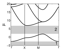
Figure 1: The band structure of the linearized equation (1) in the first Brillouin zone, for depth $\varepsilon=7.4$ of the linear lattice; $\mu$ is the chemical potential of the Bloch waves.

At $q=0$, Eq. (1) amounts to the usual model with the LL potential and spatially uniform nonlinearity. The LL and NL are commensurate at $q=2$, and the subharmonic commensurability, with the ratio of the LL and NL periods $1:2$, occurs at $q=1$. The full incommensurability (overall quasi-periodicity in the system) corresponds to irrational values of $q$, but, in practical terms, the incommensurability may be emulated by $q=1.5$, with the period ratio $3:4$. The Q1D versions of the model correspond to dropping terms $\cos\left(2\pi y\right)$ and/or $\cos\left(\pi qy\right)$ in the linear and/or nonlinear potentials.

Stationary solutions to Eq. (1) with chemical potential $\mu$ (or propagation constant $-\mu$, in terms of the guided optical waves) are looked for as $\psi(x,y,t)=\phi(x,y)\exp(-i\mu t)$, where function $\phi(x,y)$ satisfies equation

$$\mu\phi = -(1/2)\nabla^{2}\phi-\varepsilon\left[\cos(2\pi x)+\cos(2\pi y)~{}\right]\phi$$ (2)

$$-g\left[\cos(\pi qx)+\cos(\pi qy)\right]|\phi|^{2}\phi.$$

The VA will be based on the Lagrangian of Eq. (2), which is

$$L = \int_{-\infty}^{+\infty}\left\{\mu|\phi|^{2}-\frac{1}{2}|\nabla\phi|^{2}+\varepsilon\left[\cos(2\pi x)+\cos(2\pi y)\right]|\phi|^{2}\right.$$

$$\left.+\frac{g}{2}\left[\cos(\pi qx)+\cos(\pi qy)\right]|\phi|^{4}\right\}dxdy.$$

III Localized modes in the semi-infinite gap

III.1 Fundamental solitons

We start the analysis of the ordinary solitons, which are expected to exist in the semi-infinite gap at $g=+1$ in Eq. (1), using the VA based on the Gaussian ansatz, $\phi\left(x,y\right)=A\exp\left[-\left(x^{2}+y^{2}\right)/\left(2W^{2}\right)\right]$, with the corresponding norm $N\equiv\int\int\phi^{2}\left(x,y\right)dxdy=\pi\left(AW\right)^{2}$ Salerno . The substitution of the ansatz into the Lagrangian yields the following expression, written in terms of $N$ and width $W$:

$$L_{\mathrm{eff}}=\frac{N}{2}\left[\mu-\frac{1}{2W^{2}}+2\varepsilon e^{-\left(\pi W\right)^{2}}+\frac{gN}{2\pi W^{2}}e^{-\left(\pi qW\right)^{2}/8}\right],$$ (3)

and the respective variational equations, $\partial L_{\mathrm{eff}}/\partial W=\partial L_{\mathrm{eff}}/\partial N=0$:

$$\left(2\pi W^{2}\right)^{2}\varepsilon e^{-\left(\pi W\right)^{2}}+\pi^{-1}gNe^{-\left(\pi qW\right)^{2}/8}\left[1+\left(\pi qW\right)^{2}\right] = 1,$$

$$\left(2W^{2}\right)^{-1}-2\varepsilon e^{-\left(\pi W\right)^{2}}-gN\left(\pi W^{2}\right)^{-1}e^{-\left(\pi qW\right)^{2}/8} = \mu.$$ (4)

Dependences $\mu(N)$ for the soliton families, produced by a numerical solution of Eqs. (4) at different values of incommensurability index $q$, are displayed in Fig. 2, along with their counterparts, produced by numerical solutions of stationary equation (2) and verified in direct simulations of Eq. (1).

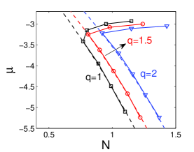
Figure 2: (Color online) The chemical potential vs. the norm for soliton families in the semi-infinite gap of the model with the full 2D linear and nonlinear potentials, as produced by the VA (dashed curves), and as found from numerical solutions of Eq. (2) (chains of symbols).

Shapes of the stable solitons generated in the semi-infinite gap by the full 2D model, and by its version with the Q1D linear potential, are displayed in Figs. 3 and 4. Naturally, these shapes are, respectively, quasi-isotropic and strongly elongated, resembling those reported previously in other 2D models stabilized by the LL potentials Salerno ; review-multiD ; Barcelona ; Abd .

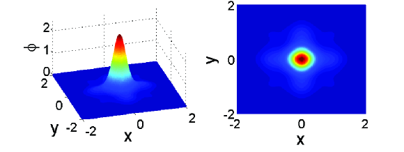
Figure 3: (Color online) A typical example of a stable fundamental soliton found in the semi-infinite gap of the model with the full 2D linear and nonlinear potentials, for $g=+1$, $q=1.5$, and $\mu=-5.24,$ $N=1.22$. The right panel shows contour plots of the stationary real wave function, $\phi\left(x,y\right)$, for the soliton.

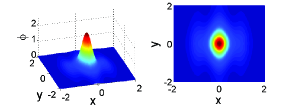
Figure 4: (Color online) The same as in Fig. 3, but in the case of the Q1D linear potential (while the nonlinear potential remains two-dimensional), for $g=+1$, $q=1$, and $\mu=-2.91,$ $N=1.68$. The shape of the solitons in the version of the model where the nonlinear potential is also made quasi-one-dimensional is quite similar  to the present one.

It is seen from Fig. 2 that the VA describes the ordinary solitons with a reasonable accuracy, except near the edge of the semi-infinite gap, where the Gaussian ansatz is irrelevant, as the soliton becomes very wide and develops a complex shape. Further, simulations of the evolution of perturbed solitons demonstrate that the stability of the solitons exactly obeys the VK criterion, $d\mu/dN<0$ [strictly speaking, if dependence $\mu(N)$ is taken in the numerically found form]. These features of the families of ordinary-soliton solutions are similar to those found before in the 1D variant of the model HS .

The stability of the 2D solitons in the semi-infinite gap, for all the four realizations of the model (2D or Q1D linear and nonlinear potentials) is summarized in Fig. 5. When solitons are unstable, they suffer decay into radiation waves (rather than rearranging themselves into stable solitons). It is worthy to note that the replacement of the full 2D NL by its Q1D counterpart leads to an expansion of the stability areas, which is explained by the fact that, in the case of the Q1D NL, the ordinary solitons should make the effort to “dodge” the destabilizing locally self-repulsive nonlinearity only in one direction, rather than in two.

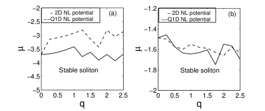
Figure 5: (a) Stability borders for the family of the ordinary solitons (in the semi-infinite gap) in the model with the 2D linear potential and 2D or Q1D nonlinear one (solid and dashed lines, respectively). (b) The same, in the case of the Q1D linear potential. The solitons are stable beneath the respective borders.

In addition to the above analysis, we tried to test the mobility of the solitons by simulating their evolution after sudden application of a “kick”, i.e., multiplication of the wave function of a stable quiescent soliton by the phase-tilt factor, $\exp\left(i\left(k_{x}x+k_{y}y\right)\right)$, with vectorial kick parameter $\mathbf{k}$. Except for the obvious case when both the LL and NL have the collinear Q1D structure, and the kick is applied in the unconfined direction, mobile solitons were not found, even if either the LL or NL potential was of the Q1D type.Instead of setting the soliton in motion, a sufficiently strong kick tends to destroy it.

III.2 Solitary vortices

Stable solitary vortices with topological charge $1$ were found as “hollow” four-peak complexes, with the separation between the peaks equal to the double period of the LL potential ($\Delta x=\Delta y=2$), and a nearly empty cell at the center of the pattern, see an example in Fig. 6. It is relatively easy to find stable vortices of this type, due to the weak interaction between the peaks. More densely packed vortex patterns can also be constructed, but we could not find stability regions for them. It is known from the studies of other models too that the vortices with inner “voids” are more likely to be stable review-multiD ; Barcelona .

Actually, the vortices are stable only for values of the incommensurability index close to $q=0,~{}1,$ and $2$—namely, within intervals of half-width $\Delta q\simeq 0.1$ around these values. The latter observation may be explained by the fact that, at such values of $q$, both the linear and nonlinear potentials have minima at or close to sites where the the power (density) peaks are located.

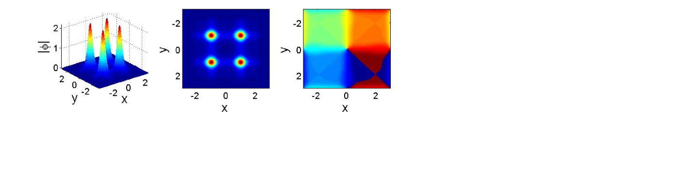
Figure 6: (Color online) An example of a stable vortex with topological charge $1$, which is supported, in the semi-infinite gap, by the combination of the full 2D linear and nonlinear structures with $q=1$ and $g=+1$. The left, middle, and right panels display, respectively, the absolute value of the field, $|\phi(x,y)|$, as a function of the coordinates, contour plots of $|\phi(x,y)|$, and the distribution of the phase, which carries the vorticity. Parameters of the vortex are $\mu=-5.1$, $N=4.4$.

Furthermore, the vortices of the type shown in Fig. 6 are found to be stable (in the semi-infinite gap) in the case when the LL potential is fully two-dimensional, while the NL may be of either 2D or Q1D type. The corresponding families of the vortex modes are represented by $\mu(N)$ curves in Fig. 7. Detailed analysis demonstrates that the stability of these families exactly follows the VK criterion, i.e., stable are portions of the families with $d\mu/dN<0$.

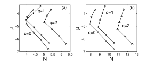
Figure 7: (Color online) The same as in Fig.2, but for families of solitary vortices in the semi-infinite gap, supported by the combination of the full 2D linear potential with the 2D (a) or Q1D (b) nonlinear lattice.

IV Gap solitons and vortices

IV.1 Fundamental solitons

Numerically generated fundamental GSs feature, as usual, more complex shapes than the ordinary solitons, see an example of a stable GS, found sufficiently far from edges of the finite bandgap, in Fig. 8 (in the model combining the 2D LL and Q1D NL, the shapes of the GSs are quite similar). The GS families are characterized by $\mu(N)$ curves which are shown in Fig. 9(a). Unlike the ordinary solitons (cf. Fig. 2), the GSs always feature $d\mu/dN>0$, thus complying with the “anti-VK” criterion proposed in Ref. HS .

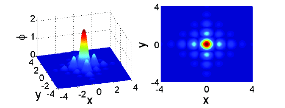
Figure 8: (Color online) A typical example of a stable gap soliton in the model with the full 2D NL, for $g=-1,q=1.5,$ and $\mu=3.4,N=1.4$.

Numerical tests demonstrate that the GSs tend to be stable sufficiently deep inside the finite bandgap, and unstable near its edges (unstable GSs suffer decay into radiation). The numerically found stability borders for the entire set of GSs in the two versions of the present model, with the full 2D NL and its Q1D counterpart, are presented in Fig. 9(b). It is observed that, on the contrary to the solitons in the semi-infinite gap, the stability region for GSs tends to be essentially narrower for the NL of the Q1D type, in comparison with the full 2D NL. The latter feature seems natural, as, unlike the case of ordinary solitons, the NL may provide for an additional support to the GSs.

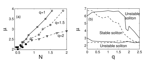
Figure 9: (a) Curves $\mu(N)$ for families of gap solitons in the model with the full 2D nonlinear potential. Black squares denote unstable solitons close to the bottom edge of the bandgap. (b) Stability borders for the entire set of the GS families in the model with the 2D and Q1D nonlinear potentials (solid and dashed lines, respectively). The solitons are stable between the corresponding stability borders. Both the top and bottom borders are located near the respective edges of the finite bandgap.

With the increase of $q$, the GS stability areas clearly tend to shrink to nil, which actually happens in Fig. 9(b) for the variant of the model with the Q1D NL (we expect the same ought to happen for the full 2D NL, but numerical problems impede extending the stability diagram to still larger values of $q$). This trend is explained by the fact that, at large $q$, the rapidly oscillating NL field tends to average itself to zero, hence the broad (see Fig. 8) GS ceases to feel the action of the nonlinearity. The ordinary solitons in the semi-infinite gap do not demonstrate such a trend (cf. Fig. 5), as, following the increase of $q$, these solitons are able to compress themselves inside a single cell of the structure, remaining centered around a region with the self-attractive nonlinearity. Finally, numerical tests demonstrate that, as well as it was concluded above for the ordinary solitons, the GSs are not mobile objects (not shown here in detail).

IV.2 Solitary vortices

Stable vortex solitons that can be found in the finite bandgap feature the same structure which supports the stable vortices in the semi-infinite gap (cf. Fig. 6), i.e., they are built of four peaks separated by the distance equal to the double LL period, the vorticity being carried by the corresponding phase distribution, see an example in Fig. 10. The difference from the situation in the semi-infinite gap is that the solitary vortices in the finite bandgap may be stable only when both LL and NL have the full 2D structure (i.e., the vortices are unstable if the NL is of the Q1D type).

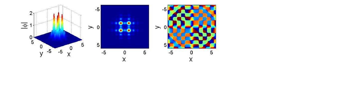
Figure 10: (Color online) An example of the stable vortex soliton found in the finite bandgap, for $q=1,$ $g=-1$ and $\mu=3.5,$ $N=5.36$. The meaning of the three panels is the same as in Fig. 6,

As well as their counterparts in the semi-infinite gap, the solitary vortices in the finite bandgap are found to be stable only for the values of incommensurability index close to $q=0,$ $1,$ and $2$. Families of these vortices are represented in Fig. 11 by the corresponding $\mu(N)$ curves. As well as the fundamental gap solitons, the stable vortices in the finite gap obey the “anti-VK criterion, $d\mu/dN>0$.

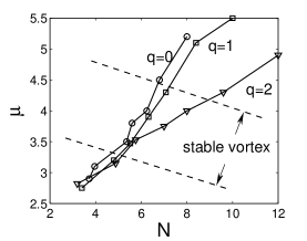
Figure 11: The dependence of the chemical potential on the norm for families of solitary vortices in the finite bandgap. Stable portions of the vortex families are located inside the marked stripe.

V Conclusions

We have introduced the model of 2D nonlinear photonic crystals and BEC based on the interplay of linear and nonlinear lattices with different (generally, incommensurate) periods, which may be considered as a “nonlinear quasicrystal”. Both fully 2D periodic potentials and their Q1D reductions were considered. For the ordinary solitons in the semi-infinite gap, the VA (variational approximation) was developed. In the general case, the solitons and solitary vortices were explored by means of numerical methods. The stability regions have been identified for the entire sets of the ordinary solitons and GSs (gap solitons). Stable families of vortex solitons of both types have been found too.

A relevant direction for the development of the analysis reported above may be search for stable higher-order vortices. On the other hand, it may also be interesting to extend the analysis to a broader parameter region, which may give rise to higher-order bandgaps, in addition to the single finite bandgap existing in the situation considered in this work, and construct solitons and solitary vortices in the additional gaps.

The work of J.Z. was supported by a postdoctoral fellowship provided by the Tel Aviv University, and by grant No. 149/2006 from the German-Israel Foundation.

References

- (1) Joannopoulos J D , Johnson S G, Winn J N and Meade R D 2008 Photonic Crystals: Molding the Flow of Light (Princeton University Press: Princeton); Skorobogatiy M and Yang J 2009 Fundamentals of Photonic Crystals Guiding (Cambridge University Press: Cambridge).
- (2) Baizakov B B, Malomed B A and Salerno M 2003 Europhys. Lett. 63 642-8; Yang J and Musslimani Z H 2003 Opt. Lett. 28 2094-6.
- (3) Baizakov B B, Konotop V V and Salerno M 2002 J. Phys. B: At. Mol. Opt. Phys. 35 5105-19; Ostrovskaya E A and Kivshar Y S 2004 Opt. Exp. 12 19-29.
- (4) Sakaguchi H and Malomed B A 2004 J. Phys. B: At. Mol. Opt. Phys. 37 2225-39; Ostrovskaya A E and Kivshar Y S 2004 Phys. Rev. Lett. 93 160405-4.
- (5) Brazhnyi V A and Konotop V V 2004 Mod. Phys. Lett. B 18 627-51; Morsch O and Oberthaler M 2006 Rev. Mod. Phys. 78 179-215.
- (6) Malomed B A, Mihalache D, Wise F and Torner L 2005 J. Optics B: Quant. Semicl. Opt. 7 R53-R72.
- (7) Kartashov Y V, Vysloukh V A, and Torner L 2009 Progress in Optics 52 63-148 (ed. by E. Wolf: North Holland, Amsterdam).
- (8) Lederer F, Stegeman G I, Christodoulides D N, Assanto G, Segev M and Silberberg Y 2008 Phys. Rep. 463 1-126.
- (9) Mayteevarunyoo T, Malomed B A and Dong G 2008 Phys. Rev. A 78 053601-12 .
- (10) Kartashov Y V, Malomed B A, and Torner L 2011 Rev. Mod. Phys. 83 247-305.
- (11) Kartashov Y V, Vysloukh V A, Szameit A, Dreisow F, Heinrich M, Nolte S, Tünnermann A, Pertsch T and Torner L 2008 Opt. Lett. 33 1120-2.
- (12) Sakaguchi H and Malomed B A 2010 Phys. Rev. A 81 013624-9.
- (13) Vakhitov M and Kolokolov A 1973 Izvestiya VUZov Radiofizika 16 1020-8 [English translation: 1973 Radiophys. Quantum. Electron. 16 783-9]; Bergé L 1998 Phys. Rep. 303 259-370.
- (14) Baizakov B B, Malomed B A and Salerno M 2004 Phys. Rev. A 70 053613-9; Mihalache D, Mazilu D, Lederer F, Kartashov Y V, Crasovan L C and Torner L 2004 Phys. Rev. E 70 055603(R)-4; Gubeskys L and Malomed B A 2009 Phys. Rev. A 79 045801-4.
- (15) Sakaguchi H and Malomed B A 2006 Phys. Rev. E 74 026601-7.
- (16) Levi L, Rechtsman M, Freedman B, Schwartz T, Manela O and Segev M 2011 Science 332 1541-4; Vardeny Z V and Nahata A 2011 Nature Photonics 5 453-3.
- (17) da Luz H L F, Abdullaev F K, Gammal A, Salerno M and Tomio L 2010 Phys. Rev. A 82 043618-8.