A Stochastic Stick - Slip Model Linking Crustal Shear Strength and Earthquake Interevent Times

Abstract

Background

The current understanding of the earthquake interevent times distribution (ITD) in terms of seismological laws or fundamental physical principles is incomplete. The Weibull distribution is used to model the earthquake ITD.

Purpose

To better understand the earthquake ITD in terms of fracture mechanics.

Method

We link the earthquake ITD on single faults with the Earth’s crustal shear strength distribution, for which we use the Weibull model, by means of a phenomenological, stochastic stick - slip model. We generalize the model for fault systems.

Results

We obtain Weibull ITD for power-law stress accumulation, i.e., $\sigma(t)=\alpha\,t^{\beta}$, where $\beta>0$ for single faults or fault systems with homogeneous strength statistics. We also show that logarithmic stress accumulation leads to the log-Weibull ITD. For the Weibull ITD, we prove that (i) $m=\beta\,m_{s}$, where $m$ and $m_{s}$ are, respectively, the interevent times and crustal shear strength Weibull moduli and (ii) the time scale $\tau_{s}=(S_{s}/\alpha)^{1/\beta}$ where $S_{s}$ is the scale of crustal shear strength. We investigate deviations of the ITD tails from the Weibull due to sampling bias, magnitude selection, and non-homogeneous strength parameters. Assuming the Gutenberg - Richter law and independence of $m$ on the magnitude threshold, $M_{L,c},$ we deduce that $\tau_{s}\propto e^{-\rho_{M}M_{L,c}},$ where $\rho_{M}\in[1.15,3.45]$ for seismically active regions. We demonstrate that a microearthquake sequence conforms reasonably well to the Weibull model.

Conclusions

The stochastic stick - slip model justifies the Weibull ITD for single faults and for homogeneous fault systems, while it suggests mixtures of Weibull distributions for heterogeneous fault systems. Non-universal deviations from Weibull statistics are possible, even for single faults, due to magnitude thresholds and non-uniform parameter values.

I INTRODUCTION

Tectonic earthquakes are the result of the stick - slip motion of plates within the Earth’s crust. This motion can be viewed in the framework of driven dissipative systems. Earthquakes are complex processes that involve nonlinearities, stochasticity, and multiple spatiotemporal scales. Earthquakes originate on individual faults, which can be viewed as the fundamental structural units for earthquake processes. Faults are geological structures that span a variety of scales, from a few centimeters up to thousands of kilometers for plate boundary faults, and accommodate earthquakes that span up to eight orders of magnitude in size Scholz (2002); Sornette (1999). Neighboring faults interact with each other leading to space-time organization of earthquakes within fault systems, e.g. Mouslopoulou and Hristopoulos (2011). The statistical laws of seismicity, e.g., the Gutenberg - Richter scaling law, are valid for systems of faults but not necessarily for single faults Serino et al. (2011).

One of the most interesting problems in statistical seismology and statistical physics is the probability distribution of the times between successive earthquake events that exceed a specified magnitude threshold, i.e., the so-called interevent times distribution. The terms return intervals, waiting times and recurrence intervals are also used instead of interevent times. A subtle but important distinction can be made between recurrence intervals, which refer to consecutive events that take place on the same fault, and interocurrence intervals, which focus on all faults in a specified region Abaimov et al. (2008). The statistical properties of recurrence intervals are more difficult to estimate, because less information is available for individual faults. The distinction is, nevertheless, conceptually important, since recurrence intervals characterize the one-body, i.e., the single-fault, problem, while interoccurrence intervals are associated with the activity of the many-body system Sornette (1999). In the following we use the term interevent times in both cases, but we distinguish between models that apply to the one-body versus the many-body problems.

Knowledge of the interevent times distribution is important for the assessment of earthquake hazard in seismically active regions. From a practical perspective, inferring interevent times statistics for very large earthquakes based on the statistics of smaller-magnitude and higher-frequency events is highly desirable. In seismology, earthquakes are categorized as foreshocks, main shocks and aftershocks. Aftershocks are assumed to be triggered by dynamic stress changes induced by the main event, such as stress redistribution, fluid flow triggering, etc., that are not directly linked to the tectonic motion of the plates. The classification of earthquakes as main events, foreshocks and aftershocks (declustering), is based on heuristic arguments. The result of declustering analysis strongly depends on the method used Luen and Stark (2011). Given this ambiguity and the fact that all seismic events in a fault system can be viewed as the result of the same dynamic process, we do not distinguish between different types of events; this approach is commonly used in statistical physics studies Bak et al. (2002); Corral (2003, 2004, 2006); Saichev and Sornette (2007).

I.1 Notation

We briefly comment on some notation and abbreviations used in the following: the probability density function of a random variable $X(t)$ is denoted by $f_{\rm X}(x)$ and the cumulative probability function by $F_{\rm X}(x)=P(X\leq x)$. The strength of the Earth’s crust is denoted by the random variable $S$, which is assumed to follow Weibull statistics with shape parameter $m_{s}$ and scale parameter $S_{s}.$ The local magnitude (Richter scale) of an earthquake event will be denoted by $M_{L}$, and the magnitude threshold by the parameter $M_{L,c}$ . The earthquake times are denoted by the random variable $t_{i}$, where the index $i$ counts the natural time (i.e. the event order), and the interevent times are denoted by $\tau_{i}=t_{i+1}-t_{i}$. Finally, $\hat{A}$ will denote the estimate of $A$ from data, where $A$ stands for a function or a distribution parameter. We also use the following abbreviations: PDF for the probability density function, CDF for the cumulative distribution function, ITD for the interevent times distribution and CSS for the Cretan seismic sequence.

I.2 Earthquake interevent times

The distributions of the magnitudes and return intervals of extreme events are research topics that attract significant interest Sornette (2004). Extreme events are usually distributed in both space and time, but herein we assume that the spatial dependence can be ignored to simplify the analysis. Let us further assume that an extreme event corresponds to excursions of a random function $X(t)$, where $t$ is the time index, to values above a specified threshold $z_{q}$. The classical extreme value theory focuses on the probability distributions of such extreme events Gumbel (1935). The Fisher-Tippet-Gnedenko theorem Fisher and Tipett (1928); Gnedenko (1943) shows that the distribution of $M_{n}:=\max(X_{1},\ldots,X_{n})$, where the $X_{i},i=1,\ldots,n$ are independent and identically distributed (i.i.d.) variables, is given by Generalized Extreme Value (GEV) distributions. The GEV include the Gumbel, reverse Weibull and Fréchet distributions. The type of GEV obtained depends on the tail behavior of the probability distribution of the $X_{i}$. Similar distributions, but with reversed supports, are obtained for minima. Extension of the classical CLTs (which involve deterministic scalings of the random variables), to randomized CLTs that enable stochastic scaling transformations have been recently proposed in Eliazar and Klafter (2010).

If the earthquakes in a fault system occurred randomly, the event times should be uniformly distributed. Uniform distribution over an unbounded time domain implies Poisson statistics as lucidly explained in Eliazar and Klafter (2010). The Poisson model leads to an exponential distribution of interevent times. It has been proposed that the earthquake times follow the Poisson distribution if foreshocks and aftershocks are removed Gardner and Knopoff (1974). Different declustering approaches have been proposed to isolate main events from aftershocks and foreshocks. Nevertheless, these approaches are not based on fundamental principles, and the results of their application on seismic data vary widely. In addition, a recent rigorous statistical analysis casts doubt on the validity of the Poisson model even for declustered data Luen and Stark (2011). The periodic model supports that the intervals between characteristic earthquakes are approximately constant Schwartz and Coppersmith (1984). This is in contrast with the observations collected from large faults globally Abaimov et al. (2008); Marco et al. (1996); Weldon et al. (2004).

Spatial and temporal inter-dependence of seismic events can explain deviations from the Poisson and the periodic models. Several research papers propose that earthquakes are self-organized systems, perhaps near a critical point Bak et al. (2002); Corral (2003); Saichev and Sornette (2007) or systems near a spinodal critical point Klein et al. (1997); Serino et al. (2011). Both cases imply the emergence of power laws in the system. Bak et al. Bak et al. (2002) introduced a global scaling law that relates earthquake interevent intervals with magnitude and distance between earthquakes. These authors analyzed seismic catalogue data from an extended area in California that includes several faults over a period of 16 years (ca. $3.35\times 10^{5}$ events). They observed power-law dependence over 8 orders of magnitude, indicating correlations over a wide range of interevent intervals, distances and magnitudes. Corral and coworkers Corral (2003, 2004, 2006); Corral and Christensen (2006) introduced a local modification of the scaling form so that the interevent time probability density function (PDF) follows the universal expression $f_{\rm\tau}(\tau)\simeq\lambda\tilde{f}(\lambda\,\tau)$, where $\tilde{f}(\tau)$ is a scaling function and the typical interevent time $\bar{\tau}$ is specific to the region of interest.

Saichev and Sornette Saichev and Sornette (2006, 2007) generalized the scaling function incorporating parameters with locally varying values. Their analysis was based on the mean-field approximation of the interevent times PDF in the epidemic-type aftershock sequence (ETAS) model. ETAS incorporates the Gutenberg-Richter dependence of frequency on magnitude, the Omori - Utsu law for the rate of aftershocks, and a similarity assumption that does not distinguish between foreshocks, main events and aftershocks (any event can be considered as a trigger for subsequent events).

In a different research vein, several studies of earthquake catalogues and simulations show that the Weibull distribution provides a better match of empirical interevent times distributions than the Poisson model Hagiwara (1974); Rikitake (1976, 1991); Sieh et al. (1989); Yakovlev et al. (2006); Abaimov et al. (2008); Hasumi et al. (2009a, b). The arguments supporting the Weibull distribution are based on empirical studies and extreme value theory. In particular, since the interevent times are determined by minima of the shear strength in the Earth’s crust, the standard Weibull model is a good candidate for their distribution. In contrast, the Gumbel distribution for minima has negative support and the Fréchet distribution has an unbounded support.

I.3 Aims and outline of this paper

In this paper we propose a stochastic stick - slip model that links the shear strength (in the following referred to as strength for brevity) distribution of faults in the Earth’s crust, the stress accumulation - relaxation process in the crust due to tectonic motion, and the earthquakes interevent times distribution. The model is formulated at the single-fault scale and is then extended to a system of faults by constructing a composite strength distribution.

A prototype physical model of stick - slip motion along single faults is the Burridge-Knopoff (BK) model Burridge and Knopoff (1967); Carlson et al. (1994); Xia et al. (2008). This model consists of a system of coupled differential equations representing the motion of $n$ point masses linked with elastic springs and subject to a velocity-dependent friction force, which is responsible for the slip instability. In contrast to the BK model, the stochastic stick - slip model proposed herein is phenomenological, since the time between events is determined by a heuristic stress accumulation function. We assume that the main stochastic component is due to the variations of the fault shear strength (or the strength across different faults in a system). Stochastic aspects of the stress accumulation function are not explicitly investigated in the following, but they obviously deserve further research.

The remainder of the paper is organized as follows: In section II we review the Weibull distribution and its applications to earthquake interevent times. In Section III we propose a stochastic stick - slip model for single faults and show that it admits interevent times distributions, including the Weibull, that depend on the time evolution of stress accumulation. In particular, we show that the Weibull is an admissible interevent times model, if (i) the crust strength distribution is Weibull with stationary and homogeneous parameters, and (ii) the stress accumulation increases with time as a power-law. We also show that deviations from the Weibull can result due to spatial non-homogeneity of the crustal strength parameters and by imposing finite magnitude thresholds on the seismic sequence. In section IV we generalize the model to interevent times for a system of faults. In Section V we investigate the ITD for a microearthquake sequence from the island of Crete (Greece) in relation to the proposed stick - slip model. Finally, Section VI involves a discussion, conclusions, and topics for further research.

II The Weibull distribution and earthquake interevent times

II.1 Properties of the Weibull distribution

The Weibull CDF, $F_{\rm\tau}(\tau)$, determining the probability that the time between two consecutive events is less than or equal to $\tau\geq 0$ is given by

$$F_{\rm\tau}(\tau)=1-\exp\left[-\left(\frac{\tau}{\tau_{s}}\right)^{m}\right],$$ (1)

where $\tau_{s}$ is the scale parameter and $m>0$ is the Weibull modulus or shape parameter. The PDF is defined by $f_{\rm\tau}(\tau)=dF_{\rm\tau}(\tau)/d\tau$ and is given by the equation

$$f_{\rm\tau}(\tau)=\frac{m}{\tau_{s}}\,\left(\frac{\tau}{\tau_{s}}\right)^{m-1}\,e^{-\left(\frac{\tau}{\tau_{s}}\right)^{m}}.$$ (2)

The survival function is the complementary cumulative probability function, i.e.,

$$R(\tau)=1-F_{\rm\tau}(\tau).$$ (3)

In the Weibull case, $R(\tau)$ is the stretched exponential function $R(\tau)=e^{-\left(\frac{\tau}{\tau_{s}}\right)^{m}}$. The function $R(\tau)$ represents the probability that no seismic event has occurred within time $\tau$ since the last event. Shape parameter values $m<1$ lead to a diverging density at $\tau=0$, and an almost exponential decay of $f_{\rm\tau}(\tau)$ as $\tau$ increases. For $m>1$ the PDF develops a single peak that becomes sharper with increasing $m$.

The hazard rate or failure rate is the rate of change for the probability of a seismic event, if time $t$ has elapsed since the last event. It is expressed by

$$H(\tau)=\frac{f_{\rm\tau}(\tau)}{1-F_{\rm\tau}(\tau)}=\frac{m}{\tau_{s}}\,\left(\frac{\tau}{\tau_{s}}\right)^{m-1}.$$ (4)

Data are graphically tested for Weibull dependence using the Weibull plot. The latter employs the fact that the double logarithm of the inverse survival function,

$$\Phi(\tau):=\log\log R^{-1}(\tau),$$ (5)

satisfies the straight line equation, $\Phi(\tau)=m\,\log(\tau)-m\,\log(\tau_{s})$ with slope equal to the Weibull modulus. If the data are drawn from the Weibull distribution, $\hat{\Phi}(\tau)$ obtained from the empirical CDF, $\hat{F}_{\tau}(\tau)$, is approximately a straight line.

II.2 The Weibull interevent times distribution

The Weibull distribution was investigated in Hagiwara (1974); Rikitake (1976, 1991) for large earthquakes at six subduction zones over the globe. In Sieh et al. (1989) the ITD of a sequence of 12 paleoearthquakes on the San Andreas fault was investigated. Yakovlev et al. Yakovlev et al. (2006) simulated million-year-long catalogues of earthquakes on major strike-slip faults in California. They found that the Weibull distribution fits the interevent times better than the lognormal and inverse Gaussian distributions.

Abaimov et al. Abaimov et al. (2007, 2008) concluded that the Weibull is a good model for real and simulated large-magnitude earthquakes on the San Andreas fault, and for a microearthquake sequence at a nearby site. These authors also emphasize the behavior of the hazard rate function of the Weibull distribution Davis et al. (1989); Sornette and Knopoff (1997); Corral (2005). At least for large-magnitude earthquakes, $H(\tau)$ is expected to increase with the interevent time. The exponential distribution has a constant $H(\tau)$ indicating lack of memory between events, while for the lognormal distribution $H(\tau)$ decreases with the interevent time. The Brownian-passage time distribution $H(\tau)$ tends to a constant with increasing interevent time. Of the various distributions considered as models of earthquake interevent times, an increasing $H(\tau)$ with time is exhibited only by the Weibull and gamma distributions (if $m>1)$. In addition, Abaimov et al. Abaimov et al. (2008) find evidence for the Weibull distribution in numerical solutions of the slider-block model introduced by Burridge and Knopoff Burridge and Knopoff (1967); Carlson and Langer (1989).

Robinson et al. Robinson et al. (2009) simulated approximately $500\ 000$ earthquakes of magnitudes between 3.8Mw and 6.6Mw (moment magnitude scale), over a period of two million years for faults in the Taupo Rift in New Zealand. These authors employed a synthetic seismicity model that is based on the Coulomb failure criterion and uses empirical data pertaining to the number of faults, fault lengths, and long-term slip rates. They found that a three-parameter Weibull distribution fits the interevent times of large earthquakes on most faults. The three-parameter Weibull survival function is given by $R(\tau)=e^{-(\tau-\tau_{0})^{m}/\tau_{s}^{m}},$ where $\tau_{0}$ is the location parameter. A finite $\tau_{0}$ implies that the PDF vanish for $\tau<\tau_{0}$. According to the analysis in Robinson et al. (2009), earthquakes within a normal fault system are correlated on a rift-wide scale over time periods of $\approx 3\mbox{kyrs}$.

Santhanam and Gantz Santhanam and Kantz (2008) investigated the return intervals of a random function $X(t)$, i.e., the times between consecutive excursions of $X(t)$ above a given threshold. They found that if $X(t)$ has long-range memory (i.e., power-law decay of correlations), the return intervals follow the Weibull distribution. Their mathematical formulation provides support for the Weibull model. Nevertheless, their approach is not based on the standard laws of seismology (i.e., Gutenberg-Richter and Omori’s law), and the values of $m$ admitted are $0<m\leq 1.$ In contrast, analysis of interevent times from seismic catalogues and simulations demonstrates that values $m>1$ also occur. In particular, for large earthquakes it is believed that the hazard rate function increases with the time since the last event, implying $m>1.$

Table 1: Weibull modulus $(m)$ values for earthquake ITD from published research based on empirical and synthetic data from various tectonic settings and system sizes. The magnitudes in column 4 are based on the moment magnitude scale (Mw) Hanks and Kanamori (1979).

$\#$ of events	$m$	Time span	Magnitude (Mw)	Type of data	System “Size”	Location	Reference
7	3,21	147 yrs	$>6$	Real	Single Fault	SAF/ Pallett Creek	Abaimov et al. (2008)
13	2,01	$\approx$2000 yrs	$>7$	Real	Single Fault	SAF/Wrightwood	Biasi et al.
13	2,91	$\approx$5 years	Mean=1.36	Real	Single Fault	SAF/San Juan Batista	Abaimov et al. (2008)
4606	1,97	1 Ma	$>7.5$	Simulation	Fault system	North SAF / S.S. faults	Yakovlev et al. (2006)
5093	1,87	1 Ma	$>7.5$	Simulation	Fault system	South SAF	Yakovlev et al. (2006)
2612	1,71	1 Ma	$>7$	Simulation	Fault system	Hayward / California	Yakovlev et al. (2006)
8174	1,42	1 Ma	$>6.8$	Simulation	Fault system	Calaveras / California	Yakovlev et al. (2006)
1913	1,32	1 Ma	$>6.7$	Simulation	Fault system	San Gabriel / California	Yakovlev et al. (2006)
1075	1,7	1 Ma	$>7.2$	Simulation	Fault system	Calaveras / California	Yakovlev et al. (2006)
7	2,9	147 yrs	$>6$	Real	Fault system	SAF / Parkfield	Working Group on California Earthquake Probabilities (2003)
7	1,5	$\approx$ 2000 yrs	$>7$	Real	Fault system	SAF/ Pallett Creek	Sieh et al. (1989)
$5\,10^{5}$	0.82-10	2 Ma	3.3-6.8	Simulation	Fault system	Taupo Rift / New Zealand	Robinson et al. (2009)
12024	0,91	82 months	$>4$	Real	Area	Okinawa/Japan	Hasumi et al. (2009b)
13678	0,79	82 months	$>4$	Real	Area	Chuetsu/Japan	Hasumi et al. (2009b)
12024	1,09	82 months	$>3.5$	Real	Area	Okinawa/Japan	Hasumi et al. (2009b)
13678	0,85	82 months	$>3.5$	Real	Area	Chuetsu/Japan	Hasumi et al. (2009b)
12024	1,43	82 months	$>3$	Real	Area	Okinawa/Japan	Hasumi et al. (2009b)
13678	1,08	82 months	$>3$	Real	Area	Chuetsu/Japan	Hasumi et al. (2009b)
12024	1,75	82 months	$>2$	Real	Area	Okinawa/Japan	Hasumi et al. (2009b)
13678	1,77	82 months	$>2$	Real	Area	Chuetsu/Japan	Hasumi et al. (2009b)
	1,7	70 years	6.9-8.4	Real	Area	Japan	Hagiwara (1974)
8	2,3	1000 yrs	7.9 -8.4	Real	Subduction margin	Nankai Trench / Japan	Rikitake (1976)
16	2,9	300 yrs	7.8 -8.4	Real	Subduction margin	Hokkaido-Kurille Trench / Japan	Rikitake (1976)
11	9,5	100 yrs	7.8 -8.7	Real	Subduction margin	Aluetian Trench / Alaska	Rikitake (1976)

Table 1 reviews published estimates of the Weibull parameters for the interevent times of various earthquake sequences, along with information pertaining to the magnitude, the size of the fault system, the location, and the duration of the seismic sequence. Note that values of $m>1$ prevail. In addition, estimates of $m$ obtained from records containing a small number of events tend to be higher than those from large sample sizes that lie in the range $0.79-1.97$. We believe that this tendency is partly due to the impact of the magnitude threshold on the ITD (also see section III.2 below). Also note that the data cover very different system sizes, from single faults to areas containing many fault systems.

III A stochastic stick - slip model for single faults

An overview of the physical processes associated with earthquakes is given by Kanamori and Brodsky Kanamori and Brodsky (2001, 2004). We develop our formalism based on this conceptual framework. Specifically, we establish connections between the shear strength distribution of the Earth’s crust, the dynamic process driving earthquake generation, and the distribution of interevent times. Tectonic earthquakes occur on fault planes due to a dynamic stick-slip process that locally accumulates stress caused by the plate motion. This stress accumulation eventually leads to crust failure and stress relaxation when the local crustal strength is exceeded. The phase of stress accumulation (loading phase) is followed by a phase of rapid stress relaxation, cf. Fig.3(b) in Kanamori and Brodsky (2004), which corresponds to the slip events. The stress accumulation - relaxation process is cyclically repeated. This model has been applied with constant stress accumulation rate and constant maximum, $\sigma_{\max},$ or residual, $\sigma_{\rm res},$ stress to explain the recurrence of large earthquakes. If both the maximum and residual stress are constant, the model predicts periodic behavior; if the initial stress is constant, the model predicts the time of the next event; if the final stress is constant, the model predicts that the longer the interevent time, the larger the magnitude of the following event Shimazaki and Nakata (1980).

III.1 On the distribution of crustal strength

Earthquakes are typically localized on faults in the Earth’s crust; hence, the strength of these structures and the applied tectonic loading determine the interevent times on single faults. Since the crust is composed of brittle material (rock), its strength is expected to follow the Weibull probability distribution Bazant et al. (2009). The Weibull distribution was derived in the framework of weakest-link theory, founded in the studies of Gumbel and Weibull on extreme-value statistics Chakrabarti and Benguigui (1997). This theory addresses the strength of brittle and quasibrittle materials in terms of the strengths of “representative volume elements” (RVEs) or links Curtin (1998); Hristopulos and Uesaka (2004); Alava et al. (2006); Pang et al. (2008); Alava et al. (2009). The material fails if the RVE with the lowest strength breaks, hence the term “weakest-link”. The concept of links is straightforward in simple systems, e.g., one-dimensional chains and fibers. In the case of more complicated structures, the links represent critical units that control the failure of the entire system.

Experimental studies on the strength of geological materials, such as rock (granite) under various types of loading (compressive, bending) provide evidence for the validity of the Weibull distribution Gupta and Bergström (1998); Amaral et al. (2008). At the same time, experimental measurements show that the crustal strength has a systematic dependence on the depth $h$ Sibson (1974); Zoback et al. (1993); Zoback and Townend (2001). Hence, for a single fault the following Weibull CDF is a useful approximation of the strength distribution at depth $h$:

$$F_{\rm S}[S;S_{s}(h)]=1-e^{-\left(\frac{S}{S_{s}(h)}\right)^{m_{s}}},$$ (6)

where $S_{s}(h)$ is the strength scale and $m_{s}$ is the strength Weibull modulus. Typical values of $m_{s}$ for laboratory measurements of rock samples range between 3 and 30 Gupta and Bergström (1998); Amaral et al. (2008).

The seismic events on a fault are distributed across different depths in the crust. The systematic dependence of crustal strength measurements on depth Aldersons et al. (2003); Zoback et al. (1993); Zoback and Townend (2001) implies that $S_{s}(h)$ increases continuously with $h$. This agrees qualitatively with the decreasing number of seismic events registered with increasing depth (c.f. Section V below).

The depth-averaged effective fault strength distribution is then given by

$$F_{\rm S}^{\ast}(S)=1-\frac{1}{h_{2}-h_{1}}\int_{h_{1}}^{h_{2}}dh\,e^{-\left(\frac{S}{S_{s}(h)}\right)^{m_{s}}},$$ (7)

where $h_{1}$ is the minimum and $h_{2}$ the maximum focal depth of the earthquake events. In Appendix A we evaluate the effective distribution for a linear dependence $S_{s}(h)=S_{0}+q\,h$, where $S_{s}(h_{1})=S_{0}$ and $S_{s}(h_{2})=S_{0}+q\,h_{2}$. It is shown that

$$F_{\rm S}^{\ast}(s)=1-\frac{1}{2m_{s}\,\lambda_{s}}\int_{u_{2}}^{u_{1}}du\,u^{-(1+1/m_{s})}\,e^{-b\,u},\quad b=s^{m_{s}},$$ (8)

where $s=S/\bar{S}$ is the normalized strength, $\delta h=2(h_{2}-h_{1})$, $\lambda_{s}=q\,\delta h/\bar{S}$ is the strength variability coefficient, and $u_{1,2}=\left(\frac{1}{1\mp\lambda_{s}}\right)^{m_{s}}.$ In Appendix A we also derive an explicit expression for the integral valid for ${m_{s}}\geq 1$ and a convergent infinite series that is valid for ${m_{s}}<1$.

In Fig. 1 we show the numerically integrated CDF $F_{\rm S}^{\ast}(s)$, as well its difference from the Weibull CDF, $F_{0}(s)=1-e^{-s^{m_{s}}}$, i.e., $\Delta F_{\rm S}^{\ast}(s)=F_{\rm S}^{\ast}(s)-F_{0}(s)$. Larger $m_{s}$ values lead to more pronounced $\Delta F_{\rm S}^{\ast}(s).$ Weibull plots of the effective strength distribution, shown in Fig. 2, reveal that for $m_{s}<1$ the linear dependence of $\Phi^{\ast}_{\rm s}(s)=\log\log\frac{1}{1-F_{\rm S}^{\ast}(s)}$ is maintained after the averaging, while $\Phi^{\ast}_{\rm s}(s)$ deviates from the linear (Weibull) dependence for $m_{s}>1.$

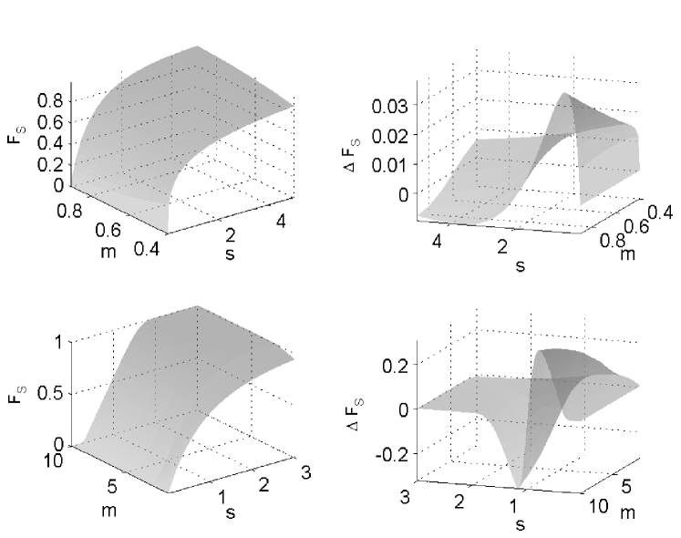
Figure 1: $F_{\rm S}^{\ast}(s)$ (top left) and $\Delta F_{\rm S}^{\ast}(s)$ (top right) for $\lambda_{s}=0.7$ and $0<m_{s}<1$. $F_{\rm S}^{\ast}(s)$ (bottom left) and $\Delta F_{\rm S}^{\ast}(s)$ (bottom right) for $\lambda_{s}=0.7$ and $10\geq m_{s}\geq 1$.

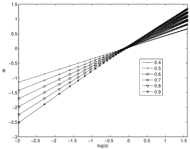
(a) $\Phi(s)$ for $0<m_{s}<1$.

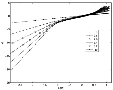
(b) $\Phi(s)$ for $10\geq m_{s}\geq 1$.

Figure 2: Weibull plots of the effective fault strength distribution based on Eq. (8).

III.2 Relation between crustal strength and ITD

The stochastic stick - slip model we propose incorporates non-uniformity of the crustal strength and links the stress accumulation and relaxation processes with the strength distribution and the earthquake interevent times.

Let us assume that $t_{i}\in[0,\tilde{t}_{i}]$ measures the time during the i-th loading phase, and that the stress increase is determined by $\sigma(t_{i})=\phi(t_{i}),$ where the loading function $\phi(t)$ is an increasing function of time. In general, the parameters of $\phi(t)$ vary randomly between different phases. For simplicity, we first assume that $\phi(t)$ is a deterministic function, the relaxation time is negligible, and the stress relaxes to a zero residual value after a seismic event. Let the random variable $\sigma(\tilde{t}_{i})$ correspond to the stress at failure for the seismic event $E_{i}$. Hence, $\sigma_{\max,i}:=\sigma(\tilde{t}_{i})$ is equal to the strength, $S_{i}$, of the crust at the particular location and time, and we can assume that it follows the Weibull distribution. The time of failure is given by $\tilde{t}_{i}=\phi^{-1}(S_{i})$, where $\phi^{-1}(\cdot)$ represents the inverse of $\phi(t)$. Once the event $E_{i}$ takes place, the stress is relaxed and the next event $E_{i+1}$ occurs when $S_{i+1}=\sigma(\tilde{t}_{i+1})$. The interevent time between events $E_{i}$ and $E_{i+1}$ is given by $\tilde{t}_{i+1}=\phi^{-1}(S_{i+1})$. In general, if the crustal shear strength $S$ is viewed as a random variable, it is related to the interevent times random variable, $\tau$, by means of $S=\phi(\tau).$

If $f_{\rm S}(S)$ is the PDF of the crust strength, and $\phi(\tau)$ is a differentiable, monotone function, the corresponding PDF of the interevent times is obtained by means of Jacobi’s theorem for univariate variable transformations as follows:

$$f_{\tau}(\tau)=f_{\rm S}(\phi(\tau))\,|\phi^{\prime}(\tau)|,$$

where $\phi^{\prime}(\tau)$ is the derivative of the loading function. In particular, if the crustal strength follows the Weibull distribution with scale parameter $S_{s}$ and modulus $m_{s}$, the ITD has a PDF that is determined by the equation

$$f_{\tau}(\tau)=m_{s}\,|\phi^{\prime}(\tau)|\,\frac{\phi(\tau)^{m_{s}-1}}{S_{s}^{m_{s}}}\,e^{-\left(\frac{\phi(\tau)}{S_{s}}\right)^{m_{s}}}.$$ (9)

III.3 Stress accumulation scenarios

III.3.1 Linear stress accumulation

Zero residual stress:

If $\phi(t)=\alpha\,\tau$, where $\alpha$ is the stress accumulation rate, it follows from Eq. (9) that the ITD is the Weibull distribution with the CDF of Eq. (1) with $\tau_{s}=S_{s}/\alpha$ and Weibull modulus $m=m_{s}$. In this scenario the stress relaxes to zero after each seismic event, c.f. Fig 3a. Since the stress accumulation rate is independent of the strength, $\tau_{s}$ and $m$ may also vary independently.

Finite residual stress:

If the stress relaxation process terminates at a non-zero residual stress, $\sigma_{\rm res}$, the loading function is given by $\phi(t)=\sigma_{\rm res}+\alpha\,t$. This scenario, illustrated in Fig. 3b, is equivalent to the elastic rebound theory developed by Reed Reid (1910); Sornette (1999); if a fault with a shear modulus $G$ and width $2b$ is sheared at constant tectonic velocity $u_{0}$, then $\alpha=G\,u_{0}/2b$. Since the residual stress does not cause failure of the crust, the crustal strength is expected to have a minimum value $S_{\min}\geq\sigma_{\rm res}$. Hence, the strength distribution corresponds to a three-parameter Weibull, the CDF of which is given by Eq. (1) with $\sigma$ replaced by $\sigma-S_{\min}.$ In this case, based on Eq. (9) the ITD becomes

$$f_{\tau}(\tau)=\frac{m}{\tau_{s}}\,\ \left(\frac{\tau-\tau_{\rm loc}}{\tau_{s}}\right)^{m-1}\,e^{-\left(\frac{\tau-\tau_{\rm loc}}{\tau_{s}}\right)^{m}},$$ (10)

where $\tau_{\rm loc}=(S_{\min}-\sigma_{\rm res})/\alpha$ is the time location parameter. If $S_{\min}=\sigma_{\rm res}$ the two-parameter Weibull model is recovered. In addition, if $S_{\min}-\sigma_{\rm res}<<S_{s}$, the two-parameter Weibull is an accurate approximation. A value of $\tau_{\rm loc}$ that is not negligible compared to $\tau_{s}$ supports the use of the three-parameter Weibull ITD model in Robinson et al. (2009).

Finite relaxation time:

The analysis above is not substantially modified if the relaxation has a finite duration $t^{\ast}_{i+1}$ (as shown schematically in Fig. 3c), and is governed by a decreasing function $\phi_{\rm rel}(t)$, since $t^{\ast}_{i+1}=(\phi_{\rm rel})^{-1}(S_{i+1})$ is also determined from the strength $S_{i+1}$. For example, assuming linear loading and relaxation relations, it follows that the stress at failure is given by $\sigma(\tilde{t}_{i+1})=\alpha\,\tilde{t}_{i+1}$ and $\sigma(\tilde{t}_{i+1})=\alpha_{\rm rel}\,\tilde{t}_{i+1}^{\ast}$. Hence, the total interevent time (measured between the zero stress values of consecutive phases) is given by $\tilde{t}_{i+1}+\tilde{t}_{i+1}^{\ast},$ which is equivalent to replacing $\alpha^{-1}$ with $\alpha^{-1}+\alpha_{\rm rel}^{-1}$. Hence, in the following we simply use $\alpha$ without loss of generality. In the case of aftershocks triggered by a main shock, the relaxation may involve a non-monotonic evolution of the stress toward its residual value. Then, $\alpha_{\rm rel}$ should be considered as an effective relaxation rate and modeled as a random variable.

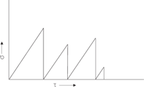
(a)

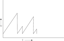
(b)

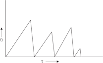
(c)

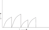
(d)

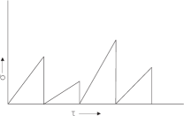
(e)

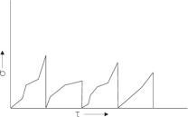
(f)

Figure 3: Schematic drawings of stress accumulation scenarios. (a) Linear loading function with zero residual stress and instantaneous relaxation. (b) Linear loading function with finite residual stress (c) Linear loading function with finite relaxation time. (d) Nonlinear loading function. (e) Linear loading function with stochastic rate. (f) Stochastic loading function.

III.3.2 Nonlinear stress accumulation

The following scenarios assume that the relaxation time is negligible and that the residual stress is zero.

Logarithmic stress accumulation:

This case is governed by a loading function $\phi(\tau)=\sigma^{\ast}\,\log(\tau/\tau_{d}),$ which implies sublinear stress evolution. According to Eq. (9), logarithmic loading leads to the log-Weibull ITD

$$f_{\tau}(\tau)=\frac{m_{s}}{\tau}\,\left(\frac{\sigma^{\ast}}{S_{s}}\right)^{m_{s}}\,\left[\log\left(\frac{\tau}{\tau_{d}}\right)\right]^{m_{s}-1}\,e^{-\left(\frac{\sigma^{\ast}\,\log(\tau/\tau_{d})}{S_{s}}\right)^{m_{s}}}.$$ (11)

An equivalent expression has been investigated in Hasumi et al. (2009a, b), where the authors employ a linear mixture of the Weibull and log-Weibull distributions to model the ITD for earthquakes in different tectonic settings. As we have shown above, the log-Weibull is justified for a sub-linear stress accumulation.

Power-law stress accumulation:

This scenario, depicted in Fig. 3d, is governed by the loading function $\phi(t)=\alpha\,\tau^{\beta},$ which leads to the Weibull ITD

$$f_{\tau}(\tau)=m\,\left(\frac{\tau}{\tau_{s}}\right)^{m-1}\,e^{-\left(\frac{\tau}{\tau_{s}}\right)^{m}},$$ (12)

where $m=m_{s}\,\beta$ and $\tau_{s}=(S_{s}/\alpha)^{1/\beta}.$ In the following, we do not distinguish between the linear and the power-law stress accumulations models since they both lead to a Weibull ITD.

Note that the relation $m=m_{s}\,\beta$ enables an indirect estimation of the loading exponent $\beta$ from the ITD Weibull modulus $m$, obtained from the analysis of the seismic event times, provided that the strength Weibull modulus is estimated from laboratory measurements. For example, if $m_{s}=10$ and $m=0.7$, it follows that $\beta=0.07.$ Let us also use the transformation $\alpha=\lambda/\tau_{0}^{\beta}$, where $\lambda$ is a constant with units of stress and $\tau_{0}$ is an arbitrary time constant. Then, it is possible to empirically determine $\lambda$. For example, if $S_{s}$ is known, e.g., $S_{s}=250$ MPa (mega Pascal), $\tau_{s}=1$day while $\tau_{0}$ is arbitrarily set to $\tau_{0}=1$sec, it follows that $\lambda=S_{s}/(\tau_{s}/\tau_{0})^{\beta}\approx 87.57$ Pa.

Stochastic stress accumulation:

In general, the statistical properties of the crust change over geological time Kanamori and Brodsky (2004). Such changes on individual faults may be due to progressive damage caused by ongoing seismic activity Serino et al. (2011). Hence, the parameters of the strength distribution may exhibit variations over time. In addition, the stress accumulation process may exhibit stochastic behavior over different time scales. For example, in the linear stress accumulation scenario the rate may fluctuate, as shown schematically in Fig. 3e. More generally, the stress accumulation may have a complex dependence with intra-phase variations of the accumulation rate as shown in Fig. 3f. In such cases, the fault is characterized by the effective ITD:

$$F_{\tau}^{\ast}(\tau;{\bm{\theta}}^{\ast})=\int_{{\bm{\theta}}_{d}}^{{\bm{\theta}}_{u}}d{\bm{\theta}}\,p({\bm{\theta}})\,F_{\tau}(\tau;{\bm{\theta}}),$$

where ${\bm{\theta}}=(\theta_{1},\ldots,\theta_{k})$ is a parameter vector with joint PDF $p({\bm{\theta}})$ that includes both strength and stress accumulation parameters. The function $p({\bm{\theta}})$ is non-negative and integrable. If all the components of ${\bm{\theta}}$ have a finite support and $F_{\tau}(\tau;{\bm{\theta}})$ is a continuous function of ${\bm{\theta}}$, it is possible to iteratively apply the first mean-value theorem of integration, which leads to

$$F_{\tau}^{\ast}(\tau;{\bm{\theta}}^{\ast})=F_{\tau}\left(\tau;\theta_{1}^{\ast}(\tau),\theta_{2}^{\ast}(\tau,\theta_{1}^{\ast}),\ldots\theta_{k}^{\ast}(\tau,\theta_{1}^{\ast},\ldots\theta_{k-1}^{\ast})\right)$$ (13)

If the dependence of the effective parameters $\theta_{i}^{\ast}$ on $\tau$ is weak, the effective CDF is of the same functional form as $F_{\tau}(\tau;{\bm{\theta}})$, with ${\bm{\theta}}$ replaced by the effective parameter vector ${\bm{\theta}}^{\ast}$ whose components are inter-dependent.

III.4 Magnitude dependence of ITD on single faults

In the following, we refer to the interevent times for the complete (i.e., including all magnitudes) seismic sequence as primitive interevent times. The main assumption in the analysis is that the primitive ITD conforms to the Weibull distribution.

III.4.1 Impact of magnitude threshold on sampled strength distribution

To link the model of repeated stress accumulation and relaxation phases with the ITD, we have assumed that all the seismic events are included, regardless of their magnitude. Then, the interevent times sample the entire crust strength distribution. In practice (see Section V), one focuses on seismic events over a threshold magnitude that varies depending on the area, the resolution of the instrumental network, and the goals of seismic risk assessment. Often the threshold magnitude is chosen as the magnitude of completeness above which all events are resolved by the observation system Woessner and Wiemer (2005).

The stress drop caused by an earthquake is related to the earthquake magnitude by means of empirical, monotonic relations Kanamori and Anderson (1975). Then, assuming that $\sigma_{\rm res}$ is constant, the threshold magnitude, $M_{L,c}$, corresponds to a unique crustal strength value $S_{c}$. Hence, the proportion of earthquakes exceeding in magnitude $M_{L,c}$ is $1-F^{\ast}_{\rm S}(S_{c})$. The sampled PDF for events with $S>S_{c}$ is given by the following equation

$$f^{\ast}_{\rm S>S_{c}}(S)=\frac{f^{\ast}_{\rm S}(S)}{1-F^{\ast}_{\rm S}(S_{c})}\,\vartheta(S-S_{c}),$$ (14)

where $\vartheta(\cdot)$ is the unit step function and the denominator normalizes the PDF. The removal of low strength values implies that the respective $\Phi(S)$ has a concave lower tail, even if the effective fault distribution $F^{\ast}_{\rm S}(S)$ is Weibull. In this respect, the impact of coarse-graining by means of a finite threshold is similar to that of non-resolved, low-magnitude events.

In Fig. 4 we show the impact of coarse-graining on a sample of Weibull random numbers with $S_{s}=100$ MPa (which is a typical average value of normal-fault strength Sibson (1974)) and $m_{s}=0.7$ with cutoffs $S_{c}=300$ KPa and $3$ MPa. In spite of the curvature of $\Phi(S)$ below the threshold, the linear part of both $\Phi(S)$ plots has the same slope, i.e., the same Weibull modulus. Nevertheless, the estimated modulus  based on the truncated sequence increases with $S_{c}$; namely, $\hat{m}_{s}\approx 0.74$ for $S_{c}=0.3$ MPa and $\hat{m}_{s}\approx 0.83$ for $S_{c}=3$ MPa. Hence, an increasing $S_{c}$ leads to an increase of the estimated Weibull strength modulus.

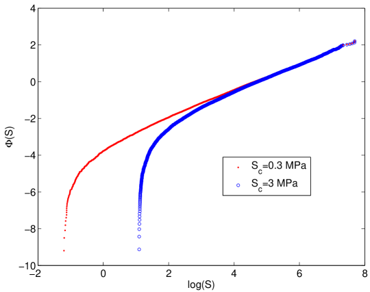
Figure 4: Plots of $\Phi(S)$ derived from a sample of 10.000 Weibull random numbers from a distribution with $S_{s}=100$ MPa and $m_{s}=0.7$ using two different thresholds ($S_{c}=300$ KPa, $3$ MPa).

III.4.2 Impact of magnitude threshold on ITD

The times between events exceeding $M_{L,c}$ extend to several stress accumulation and relaxation cycles. We assume a stress accumulation phase between events with $M_{L}\geq M_{L,c}$, such that stress increases non-monotonically between two events from a low residual value to the strength threshold that corresponds to $M_{L}$. Then, we can replace the non-monotonic dependence with an “effective” monotonically increasing stress accumulation function; e.g., in the linear case, $\alpha$ is replaced by $\alpha_{\rm eff}$. Consequently, the ITD for finite $M_{L,c}$ is also determined from Eq. (14). In general, $\alpha_{\rm eff}$ should be treated as a random variable that fluctuates depending on the number of sub-threshold events contained between the two supra-threshold events. A power-law stress accumulation function transfers to the ITD the lower-tail curvature of the crustal strength resulting from the truncation of above-threshold events.

The interevent times between events exceeding $M_{L,c}$ can be treated as sums of a randomly varying number of primitive times. To our knowledge, very little is known about sums of Weibull random numbers: a review of known results for sums of random variables reports the absence of such results for the Weibull distribution Nadarajah (2008). Recently, convergent series expansions for the PDF that governs the sum of Weibull random numbers were obtained in Yilmaz and Alouini (2009). The situation is more complicated for earthquake interevent times, since the number of summands, which is determined by the excursions of the dynamic stress above $S_{c}$, fluctuates. This coarse-graining operation completely eliminates strength values below $S_{c}$, in contrast with the summation of a fixed number of variables that shifts the mode of the distribution but does not eliminate the weight of the PDF near zero.

IV ITD of fault systems

Above, we focused on the one-body ITD problem by concentrating on single faults. Nevertheless, the seismic behavior of a given area is a many-body problem that involves multiple faults. The interevent times of a fault system are not directly obtained from the interevent times of the individual faults in the system. Let us assume that a fault $Fa$ hosts two seismic events at times $t^{Fa}_{j}$ and $t^{Fa}_{j+1}$ leading to an interevent time $\tau^{Fa}_{j}=t^{Fa}_{j+1}-t^{Fa}_{j}.$ In addition, let fault $Fb$ host two seismic events at times $t^{Fb}_{i}$ and $t^{Fb}_{i+1}$, with an interevent time $\tau^{Fb}_{i}=t^{Fb}_{i+1}-t^{Fb}_{i}.$ Next, let us assume that $t^{Fa}_{j}<t^{Fb}_{i}<t^{Fb}_{i+1}<t^{Fa}_{j+1}.$ Then, the respective interevent times for the two-fault system are $t^{Fb}_{i}-t^{Fa}_{j},\;t^{Fb}_{i+1}-t^{Fb}_{i},\;t^{Fa}_{j+1}-t^{Fb}_{i}$, which can not be obtained from $\tau^{Fa}_{j}$ and $\tau^{Fb}_{i}$.

Nevertheless, we can extend the single-fault interevent-times expressions to fault systems by assuming that all the faults are subject to a uniform stress accumulation process. Then, the same loading function applies to the entire system, and the ITD is determined from the composite strength distribution of the system . Assuming that the system involves $N$ faults characterized by $K$ different effective strength distributions $F^{\ast}_{\rm S}(S;{\bm{\theta}}_{i}),\;i=1,\ldots,K$ and that $M_{i}$ is the number of faults that follow the probability distribution $F^{\ast}_{\rm S}(S;{\bm{\theta}}_{i})$ (i.e., $M_{1}+M_{2}+\ldots M_{K}=N$), the composite strength distribution of the fault system is given by the following superposition

$${\mathcal{F}}^{\ast}_{\rm S}(S)=\sum_{i=1}^{K}p_{i}\,F^{\ast}_{\rm S}(S;{\bm{\theta}}_{i}),\quad p_{i}=\frac{M_{i}}{N},\,i=1,\ldots K.$$ (15)

A homogeneous fault system comprises faults that share the same strength distribution, $F^{\ast}_{\rm S}(S;{\bm{\theta}})$. Then, the composite strength distribution is given by ${\mathcal{F}}^{\ast}_{\rm S}(S)=F^{\ast}_{\rm S}(S;{\bm{\theta}})$.

IV.1 System with bimodal strength distribution

Let us consider a system that involves faults governed mainly by two Weibull strength distributions with different parameters, so that $K_{1}$ faults follow the first distribution, while $K_{2}=N-K_{1}$ faults follow the second. The composite strength distribution of the system is a bimodal Weibull. Let us assume that the survival function is given by the bimodal expression

$$1-{\mathcal{F}}^{\ast}_{\rm S}(S)=p\,e^{-\left(\frac{S}{S_{1}}\right)^{m_{1}}}+(1-p)\,e^{-\left(\frac{S}{S_{2}}\right)^{m_{2}}},$$ (16)

where $p=K_{1}/M$. This mixture model can lead to the “M-smile” histogram sometimes observed in the analysis of earthquake interevent times, e.g. Touati et al. (2009).

In Fig. 5 we show the histogram and corresponding empirical $\hat{\Phi}(\tau)$ for a set of $3000$ interevent times generated from the bimodal Weibull distribution with $p=2/3,$ $m_{1}=0.7$, $m_{2}=1.8$, $\tau_{1}=1.5\,10^{3}$ (sec), and $\tau_{2}=10^{5}$ (sec). The signature of bimodality is apparent as a dip in the histogram and as a saddle point in the Weibull plot. The parameters of a bimodal ITD can be estimated using the expectation-maximization algorithm Dempster et al. (1977).

The concept of a bimodal ITD has been proposed in Touati et al. (2009), where it is invoked to represent the mixing of correlated events (aftershocks) and uncorrelated (main) events. In our model, there is no a priori distinction between aftershocks and main events. However, it is conceivable that main events lead to temporary changes of the stress accumulation or the crustal strength, which imply a distinct component in the ITD linked with aftershock activity.

\begin{overpic}[width=325.215pt]{Figure5a.pdf} \put(52.0,10.0){\includegraphics[scale={.2}]{Figure5b.pdf}} \end{overpic}

Figure 5: Frequency histogram (log-log plot) and Weibull plot (inset) for $3000$ random numbers simulated from a bimodal Weibull mixture model (see text for parameters).

IV.2 Magnitude dependence of ITD for fault systems

For a single fault we showed above that the lower tail of the sampled strength PDF is cut-off (c.f. Fig 4). We expect that the abrupt change in the slope of $\Phi(S)$ at $S\approx S_{c}$ is reduced in seismic data from fault systems due to non-homogeneity of the strength parameters and possible non-stationarity caused by fluctuations in the Weibull parameters over time.

In the following, we assume that the fault-system ITD for events exceeding $M_{L,c}$ is approximated by the Weibull. The total duration of the complete seismic sequence is $T=\sum_{i=1}^{N}\tau_{i}$. Let $\overline{\tau_{1}}$ and $\overline{\tau_{2}}$ denote sample average times corresponding to truncated seismic sequences obtained for ${M}_{L,1}<{M}_{L,2},$ respectively. We assume $\overline{\tau_{1}}$ and $\overline{\tau_{2}}$ to be accurate estimates of the ensemble means of each sequence, i.e., $\overline{\tau_{1}}/\overline{\tau_{2}}\approx\mathbb{E}[\tau_{1}]/\mathbb{E}[\tau_{2}]$. If $N_{i}$ is the number of events with magnitude above ${M}_{L,i}$, then $\overline{\tau_{i}}\approx T/N_{i}$. We assume that the Gutenberg - Richter scaling, $N_{1}/N_{2}=10^{-b(M_{L,1}-M_{L,2})},$ is valid for the system. Then, it follows that

$$\frac{\overline{\tau_{2}}}{\overline{\tau_{1}}}\approx\frac{\mathbb{E}[\tau_{2}]}{\mathbb{E}[\tau_{1}]}=e^{-\rho_{M}\,(M_{L,1}-M_{L,2})},$$ (17)

where $\rho_{M}=b\,\log 10$. Since for seismically active regions $b\in[0.5-1.5]$, it follows that $\rho_{M}\in[1.15-3.45].$

The mean value of the Weibull distribution is given by $\mathbb{E}[\tau]=\tau_{s}\,\Gamma(1+1/m).$ Hence, $\tau_{s,2}/\tau_{s,1}=\mathbb{E}[\tau_{2}]\,\Gamma(1+1/m_{1})/\mathbb{E}[\tau_{1}]\,\Gamma(1+1/m_{2}).$ Then, based on Eq. (17) it follows that

$$\frac{\tau_{s,2}}{\tau_{s,1}}\approx\frac{\Gamma(1+1/m_{1})}{\Gamma(1+1/m_{2})}\,e^{-\rho_{M}\,(M_{L,1}-M_{L,2})}.$$ (18)

Equation (18) also holds for single faults that obey Gutenberg - Richter scaling and have a Weibull strength distribution.

V Analysis of Cretan Micro-Earthquake Sequences

The seismic data in the Cretan seismic sequence (CSS) investigated below are from Becker et al. Becker et al. (2010). The CSS resulted from tectonic activity generated at the Hellenic subduction margin, where the African plate is being subducted beneath the Eurasian plate; this is the seismically most active region in Europe. More than 2 500 local and regional micro-earthquake events with magnitudes up to 4.5 ${M_{L}}$ (Richter local magnitude scale) occurred during the time period between July 2003 and June 2004. The micro-earthquakes were accurately recorded by an amphibian seismic network zone onshore and offshore Crete. The network configuration consisted of up to eight ocean bottom seismometers as well as five temporary short-period and six permanent broadband stations on Crete and smaller surrounding islands (e.g. Gavdos). The magnitude of completeness varies between 1.5 $M_{L}$ on Crete and adjacent areas and 2.5 $M_{L}$ at around 100 km south of Crete. Most of the seismic activity is located offshore of central and eastern Crete (see Fig. 6). The repeat times between successive earthquake events range from 1 sec to 19.5 days.

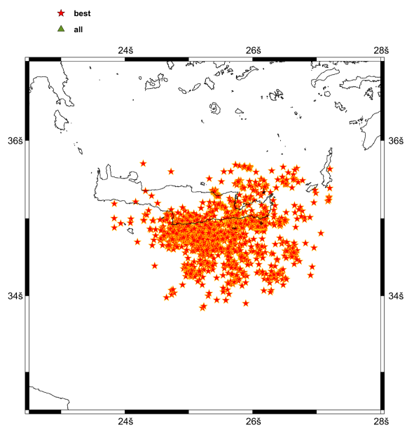
Figure 6: Map locations of CSS events (stars) on and around the island of Crete.

V.1 Exploratory analysis

The exploratory analysis of CSS includes all the events in the catalogue (magnitudes $>1M_{L}$). There is no discernible main shock in the sequence, hence declustering of the data is not considered. We use the concept of natural time to measure the ordering of the event times Abe et al. (2005); Varotsos et al. (2005): if $t_{k}$ is the time of the $k$-th event, the interevent time series in natural time is given by $\tau_{k}:=t_{k+1}-t_{k}$. The CSS interevent times series is shown in Fig. 7a, which exhibits isolated large peaks separating clusters of almost continuous seismic activity. The distribution of the earthquake focal depths is shown in Fig. 7b. Assuming a uniform tectonic stress over depth, the observed declining trend  agrees qualitatively with the reported increase of the crust strength with depth Sibson (1974); Zoback et al. (1993).

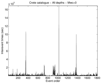
(a) CSS interevent times

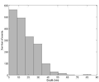
(b) CSS focal depth

Figure 7: (a) Sequence of interevent times: the horizontal axis counts the order $(i=1,\ldots,N)$ of the interval $\tau_{i}=t_{i+1}-t_{i}$, and the vertical axis measures $\tau_{i}.$ (b) Histogram of the focal depths of earthquake events.

The histogram of the magnitudes is shown in Fig. 8a. The Gutenberg - Richter law is expressed as $\log_{10}N({M_{L}}>M)=a-b\,M,$ where $N$ is the number of events with magnitude greater or equal to $M$. This implies an exponential decrease of $N$ with the magnitude, while Fig. 8a shows a non-monotonic dependence of $N$ on $M$. This is due to the resolution problem, namely the inability to observe all events with magnitudes below a critical threshold that is typically around 2 $M_{L}$ and $\approx 2.2M_{L}$ for the CSS. Setting the critical threshold at 2.2 $M_{L}$, the histogram of event frequency versus magnitude is shown in Fig. 8b. The maximum likelihood estimate of the Gutenberg - Richter exponent is $\hat{b}\approx 0.85$, i.e., within the typical range $[0.5-1.5]$ for seismically active regions.

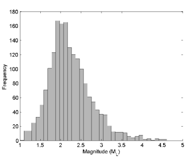
(a)

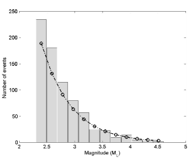
(b)

Figure 8: (a) Frequency histogram of events (complete CSS) versus magnitude. (b) Histogram of event number versus threshold magnitude and best-fit line to Gutenberg - Richter model.

The Weibull plot for CSS is shown in Fig. 9. The slope of the best-fit (minimum least squares) straight line is $\hat{m}=0.66$. Note that based on the analysis in III.2, since $\hat{m}<1$ we do not expect significant modification of the Weibull due to the depth dependence of $S_{s}$. Nevertheless, the lower tail of $\hat{\Phi}(\tau)$ is lighter than the Weibull while its upper tail is heavier. The lower tail begins roughly at $\hat{\Phi}(\tau_{1})\approx-2.5$ and the upper tail near $\hat{\Phi}(\tau_{2})\approx 1.4$. By inverting Eq. (5), we determine that $\hat{F}_{\tau}(\tau_{1})\approx 0.08$ and $\hat{F}_{\tau}(\tau_{2})\approx 0.98$. The lower-tail behavior, which involves about $8\%$ of the data, can be attributed to unresolved events (i.e., with magnitudes below the magnitude of completeness). The upper-tail behavior, which involves around $2\%$ of the data, can be partly explained due to the same effect, since failure to observe certain seismic events leads inadvertently to interevent times that are higher than in reality. The discrepancy could also be due to genuine departure of the upper ITD tail from the Weibull behavior, since the CSS data set involves a system of faults with a composite crustal strength distribution, c.f. Eq. (15).

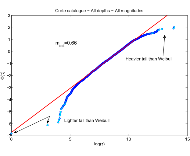
Figure 9: Weibull plot of CSS interevent times. The straight line indicates perfect Weibull dependence; $m_{est}:=\hat{m}$ is the maximum likelihood estimate of the Weibull modulus from the data.

V.2 Analysis of CSS interevent times for events above ${M}_{L,c}$

Below, we focus on interevent times between events above thresholds that exceed the magnitude of completeness. The resulting sequences are considered to be complete since they do not suffer from resolution issues. We show the Weibull plots for different magnitude thresholds in Fig. 10a. The $\hat{\Phi}(\tau;M>{M}_{L,c})$ curves show deviations from the Weibull in both the lower and upper tails. The curvature of the upper tail appears to reverse its sign as ${M}_{L,c}$ changes from 2.7 to 2.9. Nevertheless, the Weibull dependence remains a useful first approximation. In particular, for all the thresholds considered, the Kolmogorov - Smirnov test does not reject the null hypothesis that the CDF is the Weibull with the respective best-fit (maximum likelihood) parameters at significance level $5\%$.

In Table 2 we list the Weibull ITD statistics using different magnitude thresholds. Based on the confidence intervals for $\hat{m}$ in Table 2, there is no significant variation of $\hat{m}$ with ${M}_{L,c}$. In contrast, $\hat{{\rm\tau}}_{s}$ increases with ${M}_{L,c}$ as intuitively expected. In Fig. 10b we plot $\log(\hat{\tau}_{s})$ versus ${M}_{L,c}\in[2.3,3.3]$. The best-fit (minimum least squares) line passing through the data is $\log(\hat{\tau}_{s})=A-\rho_{M}\,{M}_{L,c}$ with $A=5.47,\rho_{M}=2.15$, while the $95\%$ confidence interval is $[1.76,2.54].$ The value of $\rho_{M}$ predicted by the analysis in IV.2, is $\rho_{M}^{\ast}=b\,\log(10)\approx 1.96$ in good agreement with the experimental $\rho_{M}$.

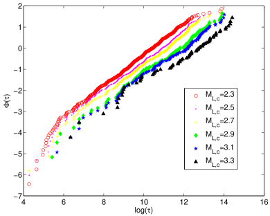
(a) CSS interevent times

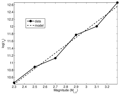
(b) CSS time scales

Figure 10: (a) Weibull plot of CSS interevent times for different magnitude thresholds. (b) Semilog plot of empirical (circles) and theoretical -according to Eq. (18)- (broken line) Weibull time scale versus ${M}_{L,c}$.

Table 2: Number of events $(N_{>})$ with magnitude above ${M}_{L,c}$ (2.3 - 3.3 ${M}_{L}$), ITD Weibull parameters $\hat{m}$ and $\hat{\tau}_{s}$ and their $95\%$ confidence intervals, $[m_{1},m_{2}]$ and $[\tau_{s,1},\tau_{s,2}]$ respectively. Weibull modulus is rounded to the second decimal place, while $\hat{\tau}_{s}$ is rounded to the third most important digit.

${M}_{L,c}$	$N_{>}$	$\hat{m}$	$\hat{\tau}_{s}$ (sec)	$[m_{1},m_{2}]$	$[\tau_{s,1},\tau_{s,2}]$
2.3	629	0.67	$3.46\,10^{4}$	[0.66, 0.74]	$[3.07\,10^{4},3.89\,10^{4}]$
2.5	415	0.70	$5.35\,10^{4}$	[0.65, 0.75]	$[4.63\,10^{4},6.18\,10^{4}]$
2.7	335	0.72	$6.80\,10^{4}$	[0.66, 0.78]	$[5.81\,10^{4},7.97\,10^{4}]$
2.9	177	0.71	$1.25\,10^{5}$	[0.63, 0.80]	$[1.04\,10^{5},1.62\,10^{5}]$
3.1	140	0.70	$1.63\,10^{5}$	[0.62, 0.80]	$[1.27\,10^{5},2.10\,10^{5}]$
3.3	70	0.67	$3.14\,10^{5}$	[0.55, 0.81]	$[2.17\,10^{5},4.56\,10^{5}]$

VI Conclusions

We propose a stochastic stick - slip model for the earthquake interevent times distribution that is based on the evolution of shear stress in the Earth’s crust and the assumption that the crust strength follows the Weibull distribution, as is common for brittle materials. The current model differs from statistical approaches that test various empirical distributions, from universal scaling laws based on the concept of criticality Bak et al. (2002); Corral (2003, 2004, 2006); Corral and Christensen (2006), from approaches rooted in probability theory Santhanam and Kantz (2008), and from stochastic branching models Saichev and Sornette (2007) that incorporate by construction the Gutenberg - Richter and Omori laws. Our model is applicable to tectonic earthquakes that are responsible for the majority of the global earthquake activity. The interevent times distribution depends on both the crustal strength and the stress accumulation models. We show that the commonly used Weibull (including the exponential) and log-Weibull interevent times distributions are derived from the stochastic stick - slip model using, respectively, power-law (including linear) and logarithmic dependence of the stress accumulation function on time. We focus on power-law stress accumulation, which leads from Weibull strength statistics to Weibull interevent times. We also demonstrate that deviations from the Weibull dependence arise due to limited resolution (i.e., sampling of events exceeding a finite magnitude threshold), and random fluctuations of the accumulation rate.

We also derive the scaling relation (18) that links the magnitude threshold with the scale of the respective Weibull interevent times distribution. This relation is based on the assumption that the Weibull model is an acceptable approximation of the ITD at finite magnitude thresholds (i.e., neglecting the lower-tail deviations) and on the Gutenberg - Richter law. The utility of the scaling relation is greater if the Weibull modulus can be assumed to remain relatively constant as the magnitude threshold changes. Then, this relation can be used to infer the Weibull time scales for larger-magnitude events based on the time scales of smaller-magnitude, more frequent, events.

In future work we will investigate dynamic stick - slip models with controlled stress accumulation rates that will allow simulating seismic events. We will also focus on the deviations from the Weibull distribution in the upper tail. Another direction that will be pursued is the interplay between empirical scaling laws of fault and earthquake parameters (e.g., fault size distribution, seismic stress drop versus fault size and earthquake magnitude) and the ITD of a fault system. In particular, a model for the behavior of a fault system should involve an average over the sizes and characteristic scales of the faults it comprises. Such an average should account for the empirical statistical facts that govern the fault population. While we believe that the interplay between the fault strength and the stress accumulation function is a universal factor controlling the ITD, the specific stress accumulation scenarios proposed and investigated herein do not exhaust the possible functional forms of stress accumulation. In particular, seismic events driven by invasion of fluids in a fault system may be generated by more local and erratic stress accumulation patterns.

Appendix A Effective strength distribution for linear depth dependence of Weibull scale parameter

We assume that the strength scale depends on the depth as $S_{s}(h)=S_{0}+q\,h.$ Then, using the variable transformation $z=\left({S_{0}+q\,h}\right)^{-m_{s}}$, and $dz=-m_{s}\,q\,(S_{0}+q\,h)^{-(m_{s}+1)}\,dh=-{m_{s}\,q}\,z^{1+1/m_{s}}\,dh,$ i.e., $dh=-\frac{dz}{m_{s}\,q}\,z^{-(1+1/m_{s})}$, the integral representing the survival function in Eq. (7) is expressed as follows

$$R_{\rm S}^{\ast}(s)=\frac{1}{m_{s}\,q\,(h_{2}-h_{1})}\int_{z_{2}}^{z_{1}}dz\,z^{-(1+1/m_{s})}\,e^{-zS^{m_{s}}},$$

where $z_{i}=(S_{0}+q\,h_{i})^{-m_{s}},i=1,2.$ We now introduce the following definitions: $2\delta h=h_{2}-h_{1}$, $\bar{S}=\frac{S_{1}+S_{2}}{2},$ and the dimensionless variables: $s=S/\bar{S}$, $\lambda_{s}=q\,\delta h/\bar{S},$ $u=z\bar{S}^{m_{s}},$ and $u_{1,2}=\left(\frac{1}{1\mp\lambda_{s}}\right)^{m_{s}}$, in terms of which the integral takes the form of Eq. (8).

A.1 Evaluation of $R_{\rm S}^{\ast}(s)$ for $m_{s}\geq 1$

We evaluate the integral in Eq. (8) using integration by parts, using the survival function $R_{\rm S}^{\ast}(s)=1-F_{\rm S}^{\ast}(s)$. This leads to

$$R_{\rm S}^{\ast}(s) =\frac{-1}{2\,\lambda_{s}}\int_{u_{2}}^{u_{1}}du\,(u^{-1/m_{s}})^{\prime}\,e^{-b\,u}$$

$$=\frac{-1}{2\,\lambda_{s}}\left[\left.(u^{-1/m_{s}}\,e^{-b\,u})\right|_{u_{2}}^{u_{1}}+b\,\int_{u_{2}}^{u_{1}}du\,u^{-1/m_{s}}\,e^{-b\,u}\right].$$

The term that originates from the boundary points (recalling that $b=s^{m_{s}}$) is equal to

$$\left[\frac{(1+\lambda_{s})}{2\,\lambda_{s}}\,e^{-\left(\frac{s}{1+\lambda_{s}}\right)^{m_{s}}}-\frac{(1-\lambda_{s})}{2\,\lambda_{s}}\,e^{-\left(\frac{s}{1-\lambda_{s}}\right)^{m_{s}}}\right].$$

For the remaining integral, we use the variable transformation $z=bu$, in terms of which we obtain

$$b\,\int_{u_{2}}^{u_{1}}du\,u^{-1/m_{s}}\,e^{-b\,u}=b^{1/m_{s}}\,\int_{z_{2}}^{z_{1}}dz\,z^{-1/m_{s}}\,e^{-z}$$

$$=b^{1/m_{s}}\,\left[\gamma(1-1/m_{s},z_{1})-\gamma(1-1/m_{s},z_{2})\right],$$

where $z_{1,2}=\left(\frac{s}{1\mp\lambda_{s}}\right)^{m_{s}}$ and $\gamma(\alpha,x)$ is the lower incomplete gamma function defined by $\gamma(\alpha,x)=\int_{0}^{x}du\,u^{\alpha-1}\,e^{-u}.$ Hence, collecting the relevant terms we obtain

$$R_{\rm S}^{\ast}(s) =\left[\frac{(1+\lambda_{s})}{2\,\lambda_{s}}\,e^{-\left(\frac{s}{1+\lambda_{s}}\right)^{m_{s}}}-\frac{(1-\lambda_{s})}{2\,\lambda_{s}}\,e^{-\left(\frac{s}{1-\lambda_{s}}\right)^{m_{s}}}\right]$$

$$-\frac{s}{2\lambda_{s}}\,\left[\gamma\left(1-\frac{1}{m_{s}},\frac{s^{m_{s}}}{(1-\lambda_{s})^{m_{s}}}\right)\right.$$

$$\left.\quad\quad\quad-\gamma\left(1-\frac{1}{m_{s}},\frac{s^{m_{s}}}{(1+\lambda_{s})^{m_{s}}}\right)\right].$$ (19)

The absolute difference between the CDF that is based on the numerical integration of Eq. (8) and that obtained from the explicit solution (A.1) is less than $1.4\times 10^{-8}$ over the parameter space of Fig. 1.

A.2 Evaluation of $R_{\rm S}^{\ast}(s)$ for $m_{s}<1$

For $m_{s}<1$ partial integration is not as efficient as for $m_{s}>1$, because the incomplete gamma function is not defined for $1-\frac{1}{m_{s}}<0$; an extension of the gamma function is possible by means of partial integration, which reduces the incomplete gamma function of a negative argument to one with a positive argument. Nevertheless, for $m_{s}<<1$ it follows that $1-\frac{1}{m_{s}}<<-1$, and repeated partial integrations are required. Alternatively, a series expansion of the integral in Eq. (8) is obtained by means of the Taylor expansion of the exponential function $e^{-b\,u}=\sum_{n=0}^{\infty}(-1)^{n}\frac{(b\,u)^{n}}{n!}$ (where $b=s^{m_{s}}$). The survival function is then given by

$$R_{\rm S}^{\ast}(s)=\frac{1}{2m_{s}\,\lambda_{s}}\sum_{n=0}^{\infty}\frac{(-1)^{n}\,s^{n\,m_{s}}}{n!}\int_{u_{2}}^{u_{1}}du\,u^{n-(1+1/m_{s})}$$

$$=\frac{1}{2\,\lambda_{s}}\sum_{n=0}^{\infty}\frac{(-1)^{n}\,s^{n\,m_{s}}}{n!}\frac{\left(1-\lambda_{s}\right)^{1-n\,m_{s}}-\left(1+\lambda_{s}\right)^{1-n\,m_{s}}}{n\,m_{s}-1}.$$ (20)

The above alternating series can be expressed as $R_{\rm S}^{\ast}(s)=\sum_{n=0}^{\infty}(-1)^{n}\,a_{n},$ where

$$a_{n}=\frac{s^{n\,m_{s}}}{n!}\frac{\left(1-\lambda_{s}\right)^{1-n\,m_{s}}-\left(1+\lambda_{s}\right)^{1-n\,m_{s}}}{2\,\lambda_{s}\,(n\,m_{s}-1)}.$$ (21)

The sequence $a_{n}$ has a maximum for an integer $n^{\ast}$ which depends on $s,\lambda_{s},m_{s}$, as shown graphically in Fig. 11.

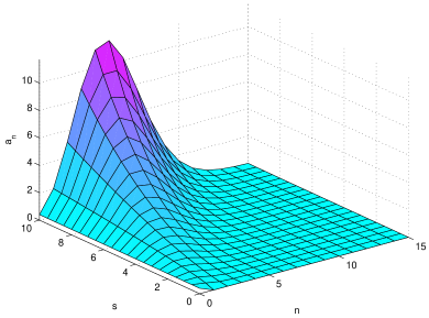
Figure 11: Dependence of the terms $a_{n}$ in Eq. (21), on $n=0,1,\ldots 15$ and $s=0,0.5,\ldots 10$, for parameter values $\lambda_{s}=0.2$, and $m_{s}=0.7$.

Fixing these three parameters, we can write $R_{\rm S}^{\ast}(s)=R_{\rm S}^{(f)}(s)+R_{\rm S}^{(in)}(s)$ where $R_{\rm S}^{(f)}(s)$ is the finite series $R_{\rm S}^{(f)}(s)=\sum_{n=0}^{n^{\ast}}(-1)^{n}\,a_{n}$ and $R_{\rm S}^{(in)}(s)=(-1)^{n^{\ast}}\sum_{n=1}^{\infty}(-1)^{n}\,{a^{\prime}}_{n},$ where ${a^{\prime}}_{n}=a_{n^{\ast}+n}$. For $n>1$ it holds that ${a^{\prime}}_{n}\leq{a^{\prime}}_{n+1}.$ Based on the alternating series test, $R_{\rm S}^{(in)}(s)$ converges. In addition, if $R_{\rm S}^{(in)}(s)$ is truncated after $M$ terms, the absolute value of the remainder is less than $a_{M+1}$. The absolute difference between the CDF that is based on the numerical integration of Eq. (8) and that obtained from the series (A.2) truncated at $n=100$ is less than $2.2\times 10^{-9}$ over the parameter space of Fig. 1.

References

- Scholz (2002) C. H. Scholz, The Mechanics of Earthquakes and Faulting, 2nd ed. (Cambridge University Press, UK, 2002).
- Sornette (1999) D. Sornette, Phys. Rep. 313, 237 (1999).
- Mouslopoulou and Hristopoulos (2011) V. Mouslopoulou and D. T. Hristopoulos, J. Geophys. Res., Ser. B 116, B07305 (2011).
- Serino et al. (2011) C. A. Serino, K. F. Tiampo, and W. Klein, Phys. Rev. Lett. 106, 108501 (2011).
- Abaimov et al. (2008) S. G. Abaimov, D. Turcotte, R. Shcherbakov, J. B. Rundle, G. Yakovlev, C. Goltz, and W. I. Newman, Pure Appl. Geoph. 165, 777 (2008).
- Luen and Stark (2011) B. Luen and P. B. Stark, “Are declustered earthquake catalogs Poisson?” (2011), http://statistics.berkeley.edu/ stark/Preprints/decluster11.pdf .
- Bak et al. (2002) P. Bak, K. Christensen, L. Danon, and T. Scanlon, Phys. Rev. Lett. 88, 178501 (2002).
- Corral (2003) A. Corral, Phys. Rev. E 68, 035102 (2003).
- Corral (2004) A. Corral, Phys. Rev. Lett. 92, 108501 (2004).
- Corral (2006) A. Corral, Phys. Rev. Lett. 97, 178501 (2006).
- Saichev and Sornette (2007) A. Saichev and D. Sornette, J. Geophys. Res., Ser. B 112, B04313/1 (2007).
- Note (1) We use the local magnitude instead of the moment magnitude since the earthquake sequence we investigate involves small to moderate size earthquakes.
- Sornette (2004) D. Sornette, Critical Phenomena in Natural Sciences (Springer, Berlin, 2004).
- Gumbel (1935) E. J. Gumbel, Ann. Inst. Henri Poincaré Probab. Stat. 5, 115 (1935).
- Fisher and Tipett (1928) M. Fisher and L. H. C. Tipett, Proc. Cambridge Philos. Soc. 24, 180 (1928).
- Gnedenko (1943) B. V. Gnedenko, Ann. Math. 40, 423 (1943).
- Eliazar and Klafter (2010) I. Eliazar and J. Klafter, Phys. Rev. E 82, 021122 (2010).
- Gardner and Knopoff (1974) J. K. Gardner and L. Knopoff, Bull. Seismol. Soc. Am. 64, 1363 (1974).
- Schwartz and Coppersmith (1984) D. P. Schwartz and K. J. Coppersmith, J. Geophys. Res. Ser. B 89, 5681 (1984).
- Marco et al. (1996) S. Marco, M. Stein, and A. Agnon, J. Geophys. Res., Ser. B 101, 6179 (1996).
- Weldon et al. (2004) R. Weldon, K. Scharer, T. Fumal, and G. Biasi, GSA Today 14, 4 (2004).
- Klein et al. (1997) W. Klein, J. B. Rundle, and C. D. Ferguson, Phys. Rev. Lett. 78, 3793 (1997).
- Corral and Christensen (2006) A. Corral and K. Christensen, Phys. Rev. Lett. 96, 109801 (2006).
- Saichev and Sornette (2006) A. Saichev and D. Sornette, Phys. Rev. Lett. 97, 078501 (2006).
- Hagiwara (1974) Y. Hagiwara, Tectonophysics 23, 313 (1974).
- Rikitake (1976) T. Rikitake, Tectonophysics 35, 335 (1976).
- Rikitake (1991) T. Rikitake, Tectonophysics 199, 121 (1991).
- Sieh et al. (1989) K. Sieh, M. Stuiver, and D. Brillinger, J. Geophys. Res., Ser. B 94, 603 (1989).
- Yakovlev et al. (2006) G. Yakovlev, D. L. Turcotte, J. B. Rundle, and P. B. Rundle, Bull. Seismol. Soc. Am. 96, 1995 (2006).
- Hasumi et al. (2009a) T. Hasumi, T. Akimoto, and Y. Aizawa, Phys. A 388, 483 (2009a).
- Hasumi et al. (2009b) T. Hasumi, T. Akimoto, and Y. Aizawa, Phys. A 388, 491 (2009b).
- Burridge and Knopoff (1967) R. Burridge and L. Knopoff, Bull. Seismol. Soc. Am. 57, 341 (1967).
- Carlson et al. (1994) J. M. Carlson, J. S. Langer, and B. E. Shaw, Rev. Mod. Phys. 66, 657 (1994).
- Xia et al. (2008) J. Xia, H. Gould, W. Klein, and J. B. Rundle, Phys. Rev. E 77, 031132 (2008).
- Abaimov et al. (2007) S. G. Abaimov, D. L. Turcotte, and J. B. Rundle, Geoph. J. Int. 170, 1289 (2007).
- Davis et al. (1989) P. M. Davis, D. D. Jackson, and Y. Kagan, Bull. Seismol. Soc. Am. 79, 1439 (1989).
- Sornette and Knopoff (1997) D. Sornette and L. Knopoff, Bull. Seismol. Soc. Am. 87, 789 (1997).
- Corral (2005) A. Corral, Phys. Rev. E 71, 017101 (2005).
- Carlson and Langer (1989) J. M. Carlson and J. S. Langer, Phys. Rev. A 40, 6470 (1989).
- Robinson et al. (2009) R. Robinson, A. Nicol, J. J. Walsh, and P. Villamor, J. Geophys. Res., Ser. B 114, B12306, 13P (2009).
- Santhanam and Kantz (2008) M. S. Santhanam and H. Kantz, Phys. Rev. E 78, 051113 (2008).
- Hanks and Kanamori (1979) T. C. Hanks and H. Kanamori, J. Geophys. Res. 84, 2348 (1979).
- (43) G. P. Biasi, R. J. Weldon, T. E. Fumal, and G. G. Seitz, Bull. Seismol. Soc. Am. 92, 2761.
- Nadeau et al. (1995) R. M. Nadeau, W. Foxall, and T. V. McEvilly, Science 267, 503 (1995).
- Working Group on California Earthquake Probabilities (2003) Working Group on California Earthquake Probabilities, “Earthquake probabilities in the San Francisco bay region: 2002 -2031,” http://pubs.usgs.gov/of/2003/of03-214/ (2003).
- Kanamori and Brodsky (2001) H. Kanamori and E. E. Brodsky, Phys. Today 54, 34 (2001).
- Kanamori and Brodsky (2004) H. Kanamori and E. E. Brodsky, Rep. Progr. Phys. 67, 1429 (2004).
- Shimazaki and Nakata (1980) K. Shimazaki and T. Nakata, Geophys. Res. Lett. 7, 279 (1980).
- Bazant et al. (2009) Z. P. Bazant, J.-L. Le, and M. Z. Bazant, Proc. Natl. Acad. Sci. U.S.A. 1061, 11484 (2009).
- Chakrabarti and Benguigui (1997) B. K. Chakrabarti and L. G. Benguigui, Statistical physics of fracture and breakdown in disordered systems (Clarendon Press, Oxford, UK, 1997).
- Curtin (1998) W. A. Curtin, Phys. Rev. Lett. 80, 1445 (1998).
- Hristopulos and Uesaka (2004) D. T. Hristopulos and T. Uesaka, Phys. Rev. B 70, 064108 (2004).
- Alava et al. (2006) M. J. Alava, K. V. V. N. Phani, and S. Zapperi, Adv. Phys. 55, 349 (2006).
- Pang et al. (2008) S.-D. Pang, Z. Bažant, and J.-L. Le, Int. J. Fract. 154, 131 (2008).
- Alava et al. (2009) M. J. Alava, K. V. V. N. Phani, and S. Zapperi, J. Phys. D 42, 214012 (2009).
- Gupta and Bergström (1998) V. Gupta and J. Bergström, J. Geophys. Res., Ser. B 103, 23875 (1998).
- Amaral et al. (2008) P. M. Amaral, J. C. Fernandes, and L. G. Rosa, Rock Mech. Rock Eng. 41, 917 928 (2008).
- Sibson (1974) R. H. Sibson, Nature 249, 542 (1974).
- Zoback et al. (1993) M. D. Zoback, R. Apel, J. Baumgärtner, M. Brudy, R. Emmermann, B. Engeser, K. Fuchs, W. Kessels, H. Rischmüller, F. Rummel, and L. Vernik, Nature 365, 633 (1993).
- Zoback and Townend (2001) M. D. Zoback and J. Townend, Tectonophysics 336, 19 (2001).
- Aldersons et al. (2003) F. Aldersons, Z. Ben-Avraham, A. Hofstetter, E. Kissling, and T. Al-Yazjeen, Earth Planet. Sci. Lett. 214, 129 (2003).
- Reid (1910) H. Reid, The mechanics of the earthquake, The California Earthquake of April 18, 1906: Report of the State Earthquake Investigation Commission 87, C192 (Carnegie Institution of Washington Publication, 1910).
- Woessner and Wiemer (2005) J. Woessner and S. Wiemer, Bull. Seismol. Soc. Am. 95, 684 698 (2005).
- Kanamori and Anderson (1975) H. Kanamori and D. Anderson, Bull. Seismol. Soc. Am. 65, 1073 (1975).
- Note (2) The Matlab maximum likelihood estimator is used.
- Nadarajah (2008) S. Nadarajah, Acta Appl. Math. 103, 131 (2008), 10.1007/s10440-008-9224-4.
- Yilmaz and Alouini (2009) F. Yilmaz and M.-S. Alouini, in Proceedings the 2009 Int. Conference on Wireless Communications and Mobile Computing: Connecting the World Wirelessly, IWCMC ’09 (ACM, New York, NY, USA, 2009) pp. 247–252.
- Note (3) This assumption is not valid if the stress accumulation is driven by fluid diffusion in the fault system.
- Touati et al. (2009) S. Touati, M. Naylor, and I. G. Main, Phys. Rev. Lett. 102, 168501 (2009).
- Dempster et al. (1977) A. P. Dempster, N. M. Laird, and D. B. Rubin, J. R. Statist. Soc., Ser. B 39, 1 (1977).
- Becker et al. (2010) D. Becker, T. Meier, M. Bohnhoff, and H.-P. Harjes, J. Seismolog. 14, 369 (2010).
- Abe et al. (2005) S. Abe, N. V. Sarlis, E. S. Skordas, H. K. Tanaka, and P. A. Varotsos, Phys. Rev. Lett. 94, 170601 (2005).
- Varotsos et al. (2005) P. A. Varotsos, N. V. Sarlis, H. K. Tanaka, and E. S. Skordas, Phys. Rev. E 71, 032102 (2005).
- Note (4) Depending on the bin size selected, the number of events may not decrease monotonically, but the overall declining trend persists.