Implementing general measurements on linear optical and solid-state qubits

Abstract

We show a systematic construction for implementing general measurements on a single qubit, including both strong (or projection) and weak measurements. We mainly focus on linear optical qubits. The present approach is composed of simple and feasible elements, i.e., beam splitters, wave plates, and polarizing beam splitters. We show how the parameters characterizing the measurement operators are controlled by the linear optical elements. We also propose a method for the implementation of general measurements in solid-state qubits.

I Introduction

The description of measurement in quantum mechanics vonNeumann:1955 ; Davies:1976 ; Kraus:1983 ; Peres:1993 is formulated as an operation to extract information from a quantum system. This operation causes a disturbance to the system. This means that the measurement accuracy (or the amount of information extracted from the system) is closely related to the back-action Braginsky;Khalili:1992 ; Banaszek:2001 ; Ozawa:2004 ; Clerk;Schoelkopf:2010 ; Wiseman;Milburn:2010 . This is a curious feature of measurement processes in quantum mechanics. Such a character is actively used in measurement-based methods for quantum engineering (e.g., Refs. Nakazato;Yuasa:2003 ; Koashi;Ueda:1999 ; Korotkov;Keane:2010 ; Ashhab;Nori:2010 ; Paraoanu:2011:EPL ; Paraoanu:2011:FP ; Ota;Nori ).

A general (or weak) measurement is associated with a positive-operator valued measure (POVM) Davies:1976 . A POVM on a measured quantum system can be expressed as a projection-valued measure in an extended system including the target system and an ancillary (or probe) system, as seen in, e.g., Ref. Peres:1993 . Therefore, we may construct arbitrary measurements from von Neumann measurements on the extended system. However, this statement does not give a specific and simple recipe to design measurement operators. Hence, a systematic approach to realize this general idea in specific physical systems is highly desirable.

A large number of experimental studies on general measurements have been performed. Huttner et al. Huttner;Gisin:1996 discriminated with two nonorthogonal states. Gillett et al. Gillett;White:2010 demonstrated quantum feedback control for a photonic polarization qubit. A polarizing beam splitter with a tunable reflection coefficient was used on the above-mentioned two experiments. Kwiat et al. Kwiat;Gisin:2001 implemented an entanglement concentration protocol with a partial-collapse measurement in a photonic qubit. Kim et al. Kim;Kim:2009 demonstrated a reversal operation of a weak measurement for a photonic qubit. The key idea in the two experiments is to use Brewster-angle glass plates. Katz et al. Katz;Korotkov:2008 performed a conditional recovery of a quantum state with a partial-collapse measurement in Josephson phase qubits. Iinuma et al. Iinuma;Hofmann:2011 studied the observation of a weak value. Kocsis et al. Kocsis;Steinberg:2011 examined a photon’s “trajectories” through a double-slit interferometer with weak measurements of the photon momentum.

In this paper, we show a method to implement general measurements on a single qubit, including both von Neumann and weak measurements. We mainly focus on a linear optical qubit. Depending on the path degree of freedom in an interferometer, a polarization state is transformed by a non-projective positive operator. We develop the idea proposed in Ref. Iinuma;Hofmann:2011 and give a systematic prescription for designing various measurement operators. The present approach is composed of simple and basic linear optical elements, i.e., beam splitters, wave plates, and polarizing beam splitters. We show how the parameters characterizing the measurement operators (e.g., the measurement strength) can be tuned. Furthermore, we show a method for implementing general measurements on a solid-state qubit.

The paper is organized as follows. In Sec. II, we show the basic idea for constructing general measurements on linear optical qubits. The notation used in this paper is explained, there. In Sec. III, we propose systematic approaches for implementing measurement operators. These method are simple and could be implementable in experiments. In addition, in Sec. IV, we study how a general measurement can be implemented in solid-state qubits. Section V is devoted to a summary of the ideas and the results.

II Setting

Let us consider a linear optical system with $N$ input and $N$ output modes. The following arguments are also applicable to other physical systems such as neutron interferometers Sponar;Hasagawa:2010 . The annihilation (creation) operator in the $n$th input mode is defined as $\hat{a}_{{\rm in},n}$ ($\hat{a}_{{\rm in},n}^{\dagger}$) with $n=1,\,2,\ldots,N$. The vacuum $|0\rangle$ is defined as $\hat{a}_{{\rm in},n}|0\rangle=0$. The bosonic canonical commutation relations are $[\hat{a}_{{\rm in},m},\hat{a}_{{\rm in},n}^{\dagger}]=\delta_{nm}$ and $[\hat{a}_{{\rm in},m},\hat{a}_{{\rm in},n}]=[\hat{a}_{{\rm in},m}^{\dagger},\hat{a}_{{\rm in},n}^{\dagger}]=0$. Similarly, we define the annihilation (creation) operator in the $n$th output mode as $\hat{a}_{{\rm out},n}$ ($\hat{a}_{{\rm out},n}^{\dagger}$). A single photon with arbitrary polarization enters the system from the first input mode. The polarization is described by a vector $|\psi\rangle\in\mathbb{C}^{2}$, with $\langle\psi|\psi\rangle=1$. We assume that the input state is a pure state $|\Psi\rangle=|\psi\rangle\otimes\hat{a}_{{\rm in},1}^{\dagger}|0\rangle$. In this setting, the photon polarization is measured, using the path degree of freedom in the interferometer as an ancillary qubit. We note that the arguments in this section can be straightforwardly extended to the case of a mixed initial state of polarization.

We calculate the photon state at each output mode. The field operators at the output modes are related to the input modes via a linear canonical transformation vanHemmen:1980 ; Umezawa:1993 ; Loudon:2000 ; Kok;Milbrun:2007 because the system is composed of linear optical elements (e.g., beam splitters). The polarization of the photon at the $n$th output mode is described by $|\phi_{n}\rangle=\langle 0|\hat{a}_{{\rm out},n}|\Psi\rangle$. Thus, we find that in terms of the output mode operators the photon state is written as $|\Psi^{({\rm out})}\rangle=\sum_{n=1}^{N}|\phi_{n}\rangle\otimes\hat{a}_{{\rm out},n}^{\dagger}|0\rangle$. Since we assume that there is no photon loss, we have $\langle\Psi^{\rm out}|\Psi^{\rm out}\rangle=\langle\Psi|\Psi\rangle$. The linearity of the system indicates that there exist linear operators $\hat{X}_{n}$ on $\mathbb{C}^{2}$ such that $|\phi_{n}\rangle=\hat{X}_{n}|\psi\rangle$. The normalization condition $\langle\Psi|\Psi\rangle=1$ implies that $\sum_{n=1}^{N}\hat{X}_{n}^{\dagger}\hat{X}_{n}=\hat{I}_{2}$, where the identity operator on $\mathbb{C}^{2}$ is $\hat{I}_{2}$. Therefore, we find that the initial state $|\psi\rangle$ is transformed by a linear operator which is related with an element of a POVM.

It is convenient for designing various kinds of POVM to add another linear optical system to some of the output modes in the interferometer before the photon detection. For example, let us set wave plates in each output mode. The wave plates in the $n$th mode describe a unitary gate $V_{n}$ given as the unitary part of $\hat{X}_{n}$. Using the right-polar decomposition Horn;Johnson:1985 , we find that $\hat{X}_{n}=\hat{V}_{n}^{\dagger}\hat{M}_{n}$, where $\hat{M}_{n}=(\hat{X}_{n}^{\dagger}\hat{X}_{n})^{1/2}$ is a positive operator. The role of the wave plates is to remove the effect of the unitary evolution $\hat{V}_{n}^{\dagger}$ from $\hat{X}_{n}$. Using the application of such “path-dependent” unitary operators, we find that $|\Psi^{(\rm out)}\rangle\to\sum_{n=1}^{N}|\psi_{n}\rangle\otimes\hat{a}_{{\rm out},n}^{\dagger}|0\rangle$, where $|\psi_{n}\rangle=\hat{V}_{n}|\phi_{n}\rangle=\hat{M}_{n}|\psi\rangle$. The measurement operators $\hat{M}_{n}$ satisfy $\sum_{n=1}^{N}\hat{M}_{n}^{\dagger}\hat{M}_{n}=\hat{I}_{2}$. Thus, we have the measurements corresponding to the POVM $\{\hat{E}_{n}\}_{n=1}^{N}$ with $\hat{E}_{n}=\hat{M}_{n}^{\dagger}\hat{M}_{n}$. The positive operator $\hat{M}_{n}$ is the essential part (i.e., the back-action associated with the measurement) of non-unitarity of $\hat{X}_{n}$ and called minimally-disturbing measurement, following Ref. Wiseman;Milburn:2010 . Throughout this paper, we will focus on such minimally-disturbing measurements.

Let us characterize the measurement operators $\hat{M}_{n}$. We can expand $\hat{M}_{n}$ as $\hat{M}_{n}=\sum_{i=1}^{2}m_{n,i}|m_{n,i}\rangle\langle m_{n,i}|$, with the eigenvalues $m_{n,i}\,(\geq 0)$ and the associated eigenvectors $|m_{n,i}\rangle$. The eigenvalues are related to the measurement strength, while the eigenvectors are regarded as the measurement direction. Let us consider the case when $m_{n,1}=1$ and $m_{n,2}=0$, for example. We find that $\hat{M}_{n}$ is a projection operator (i.e., a sharp measurement) in the direction of $\vec{m}_{n,1}$, where $\vec{m}_{n,1}$ is the Bloch vector corresponding to $|m_{n,1}\rangle\langle m_{n,1}|$. The indistinguishability between the elements of a POVM is characterized by the Hilbert-Schmidt inner product $\mbox{Tr}\,\hat{E}_{n}^{\dagger}\hat{E}_{m}$ for $n\neq m$. The elements of a projection-valued measure are distinguishable (i.e., the inner products are zero), for example. Now, we pose the question: How are these measurement features controlled by typical linear optical devices? We will answer this question in the next section.

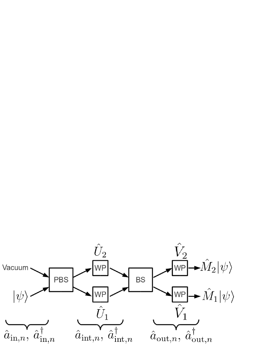
Figure 1: Schematic diagram of a proposal for implementing symmetric, arbitrary-strength two-outcome measurements on a single-photon’s polarization. This setup is essentially equal to the one in Ref. Iinuma;Hofmann:2011 . Three kinds of field operators (i.e., $\hat{a}_{{\rm in},n}$, $\hat{a}_{{\rm int},n}$, and $\hat{a}_{{\rm out},n}$) are needed for representing the path degrees of freedom. A single photon with arbitrary polarization (described by $|\psi\rangle$) enters a polarizing beam splitter (PBS). Next, the polarization is transformed by a wave plate (WP) in each arm. Then, the two arms are recombined in a beam splitter (BS). After performing unitary gates $\hat{V}_{1}$ and $\hat{V}_{2}$ for compensation purposes, the resultant polarization states are expressed in terms of the measurement operators $\hat{M}_{1}$ and $\hat{M}_{2}$ given in Eqs. (1) and (2).

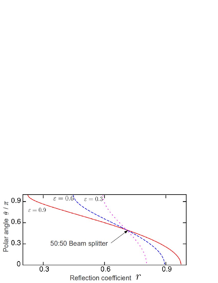
Figure 2: (Color online) Measurement direction of the measurement operators (1) and (2) for the measurement strength $\varepsilon=0.9$ (red solid), $0.6$ (blue dashed), and $0.3$ (magenta dotted). The horizontal axis represents the reflection coefficient $r$ of the beam splitter, while the vertical axis is the polar angle $\theta$ of the measurement direction. All curves merge at $(r,\,\theta)=(1/\sqrt{2},\,\pi/2)$. This case corresponds to the use of a $50:50$ beam splitter in Fig. 1.

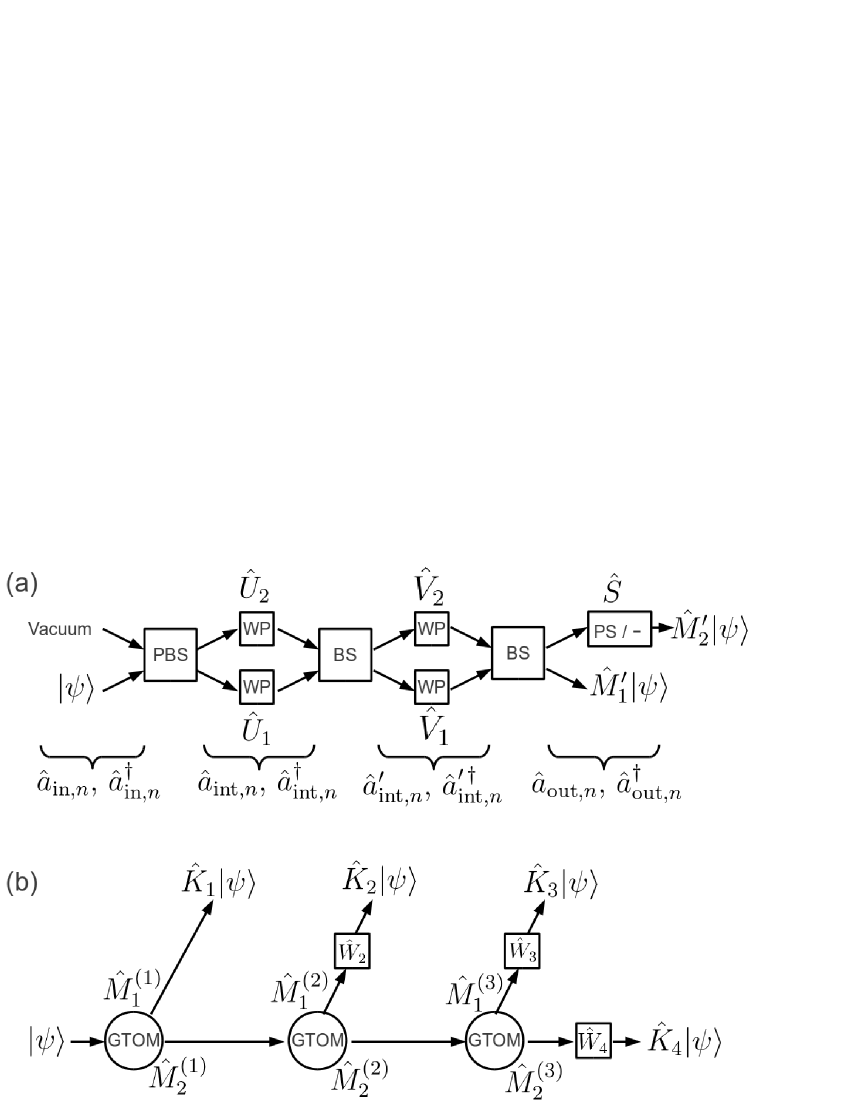
Figure 3: Schematic diagrams of the construction for general measurements with (a) two outcomes and (b) $N$ outcomes ($N=4$). In (a), the interferometer for a symmetric arbitrary-strength two-outcome measurement followed by a beam splitter leads to general two-outcome measurements. The final box leading to $\hat{M}_{2}^{\prime}|\psi\rangle$ after the last beam splitter represents a unitary gate for compensation purposes. Depending on system’s parameters, this unitary gate becomes either a phase-shift gate or the identity operator (i.e., does nothing). In (b), the repeated application of general two-outcome measurements (GTOM) allows the construction of a POVM with multiple outcomes.

III Design of general measurements on linear optical qubits

III.1 Symmetric arbitrary-strength two-outcome measurements

Let us first define a special class of general measurements, which is the target operation in this subsection. We consider a symmetric two-outcome POVM in $\mathbb{C}^{2}$ composed of convex combinations of two orthogonal projection operators

$$\hat{M}_{1}=\sqrt{\frac{1+\varepsilon}{2}}|m_{+}\rangle\langle m_{+}|+\sqrt{\frac{1-\varepsilon}{2}}|m_{-}\rangle\langle m_{-}|,$$ (1)

$$\hat{M}_{2}=\sqrt{\frac{1-\varepsilon}{2}}|m_{+}\rangle\langle m_{+}|+\sqrt{\frac{1+\varepsilon}{2}}|m_{-}\rangle\langle m_{-}|,$$ (2)

with $0\leq\varepsilon\leq 1$ and $\langle m_{+}|m_{-}\rangle=0$. Adjusting a real parameter $\varepsilon$ allows arbitrary measurement strength. We find that if the coefficient for $|m_{+}\rangle\langle m_{+}|$ increases, then the one for $|m_{-}\rangle\langle m_{-}|$ decreases, and vice versa. Thus, these measurement operators are symmetric or balanced with respect to the parameter $\varepsilon$. We call the measurements described by these linear operators symmetric arbitrary-strength two-outcome measurments (SASTOM) on $\mathbb{C}^{2}$. The disturbance induced by a SASTOM is considered to be minimum, as shown in Ref. Banaszek:2001 . Another important property of a SASTOM is $\mbox{Tr}\,\hat{M}_{1}^{\dagger}\hat{M}_{1}=\mbox{Tr}\,\hat{M}_{2}^{\dagger}\hat{M}_{2}=1$. An application of a SASTOM to quantum protocols is shown in, e.g., Ref. Ota;Nori .

Now, we propose a systematic way to construct this measurement. Let us consider an interferometer with two input and two output modes, as shown in Fig. 1. A single photon enters a polarizing beam splitter Meschede:2007 from the first input mode. Subsequently, its polarization at each arm is transformed by wave plates. Then, the two modes are recombined in a beam splitter. This system is essentially the same as in Ref. Iinuma;Hofmann:2011 . We reformulate the construction manner of a SASTOM in Ref. Iinuma;Hofmann:2011 and extend it to make more general types of measurements. Unlike the proposal in Ref. Iinuma;Hofmann:2011 , our proposals use beam splitters with tunable reflection coefficients.

Let us apply the basic idea in Sec. II to this interferometer. We need three kinds of field operators for describing the path degrees of freedom, i.e., input, intermediate, and output field operators, as shown in Fig. 1. We have an initial pure state

$$|\Psi^{({\rm in})}\rangle=|\psi\rangle\otimes\hat{a}_{{\rm in},1}^{\dagger}|0\rangle,\quad|\psi\rangle=c_{\rm H}|{\rm H}\rangle+c_{\rm V}|{\rm V}\rangle,$$

with the horizontal polarization state $|\rm H\rangle$ and the vertical polarization state $|\rm V\rangle$. The field operators $\hat{a}_{{\rm int},n}$ and $\hat{a}_{{\rm int},n}^{\dagger}$ at the output modes of the polarizing beam splitter are related to $\hat{a}_{{\rm in},n}$ and $\hat{a}_{{\rm in},n}^{\dagger}$ via $\hat{a}_{{\rm int,H},1}=\hat{a}_{{\rm in,H},1}$, $\hat{a}_{{\rm int,H},2}=\hat{a}_{{\rm in,H},2}$, $\hat{a}_{{\rm int,V},1}=\hat{a}_{{\rm in,V},2}$, and $\hat{a}_{{\rm int,V},2}=\hat{a}_{{\rm in,V},1}$ Kok;Milbrun:2007 , where $\hat{a}_{{\rm in,H},1}=|{\rm H}\rangle\langle{\rm H}|\otimes\hat{a}_{{\rm in},1}$, etc. After the single photon passes through the polarizing beam splitter, we find that the photon state is written as $|\Psi^{({\rm int})}\rangle=|u_{1}\rangle\otimes\hat{a}_{{\rm int,}1}^{\dagger}|0\rangle+|u_{2}\rangle\otimes\hat{a}_{{\rm int,}2}^{\dagger}|0\rangle$ with $|u_{1}\rangle=c_{\rm H}|{\rm H}\rangle$ and $|u_{2}\rangle=c_{\rm V}|{\rm V}\rangle$. We remark that the polarizing beam splitter produces entanglement between the polarization and the path degrees of freedom in the interferometer. Next, we perform unitary operations for the polarization on each of these intermediate modes with the wave plates. The use of half- and quarter-wave plates allows the construction of arbitrary elements of $\mbox{SU}(2)$  Simon;Mukunda:1990 ; Bhadari;Dasgupta:1990 . Hence, using the path-dependent wave plates, we find that

$$|\Psi^{(\rm int)}\rangle\to\sum_{n=1}^{2}\hat{U}_{n}|u_{n}\rangle\otimes\hat{a}_{{\rm int,}n}^{\dagger}|0\rangle,$$

with $\hat{U}_{n}\in\mbox{SU}(2)$. The canonical transformation associated with the beam splitter Loudon:2000 ; Kok;Milbrun:2007 is $\hat{a}_{{\rm out},1}=r\hat{a}_{{\rm int,}1}+t\hat{a}_{{\rm int,}2}$ and $\hat{a}_{{\rm out},2}=t\hat{a}_{{\rm int,}1}-r\hat{a}_{{\rm int,}2}$, where $r^{2}+t^{2}=1$ and $0\leq r,t\leq 1$. After the single photon passes through the beam splitter, we find that the photon state is expressed by

$$|\Psi^{(\rm out)}\rangle=\sum_{n=1}^{2}|\phi_{n}\rangle\otimes\hat{a}_{{\rm out},n}^{\dagger}|0\rangle,$$

where $|\phi_{1}\rangle=r\hat{U}_{1}|u_{1}\rangle+t\hat{U}_{2}|u_{2}\rangle$ and $|\phi_{2}\rangle=t\hat{U}_{1}|u_{1}\rangle-r\hat{U}_{2}|u_{2}\rangle$. We find that the linear operators satisfying $|\phi_{n}\rangle=\hat{X}_{n}|\psi\rangle$ are $\hat{X}_{1}=r\hat{U}_{1}|{\rm H}\rangle\langle{\rm H}|+t\hat{U}_{2}|{\rm V}\rangle\langle{\rm V}|$ and $\hat{X}_{2}=t\hat{U}_{1}|{\rm H}\rangle\langle{\rm H}|-r\hat{U}_{2}|{\rm V}\rangle\langle{\rm V}|$. The positive operators associated with $\hat{X}_{1}$ and $\hat{X}_{2}$ are given, respectively, by Eqs. (1) and (2) with

$$\varepsilon=\sqrt{1-4r^{2}t^{2}(1-|w|^{2})},\quad w=\langle{\rm H}|\hat{U}_{1}^{\dagger}\hat{U}_{2}|{\rm V}\rangle.$$ (3)

The definition of $w$ implies that the choice of the unitary gates $\hat{U}_{1}$ and $\hat{U}_{2}$ is not unique for constructing the measurement operators $\hat{M}_{n}$. For example, one can set $\hat{U}_{1}$ as the identity operator and still obtain any desired value of $w$ by adjusting $\hat{U}_{2}$. Iinuma et al. Iinuma;Hofmann:2011 set $\hat{U}_{1}=\hat{U}_{2}^{\dagger}$, which results in a real value for $w$ and thus imposes a constraint on the measurement operators that can be constructed. The range of $|w|$ is $0\leq|w|\leq 1$ since $w$ is an off-diagonal element of a unitary operator. The basis vectors $|m_{+}\rangle$ and $|m_{-}\rangle$ for $w\neq 0$ are

$$|m_{+}\rangle=\cos\frac{\theta}{2}|{\rm H}\rangle+e^{-i\phi/2}\sin\frac{\theta}{2}|{\rm V}\rangle,$$ (4)

$$|m_{-}\rangle=-e^{i\phi/2}\sin\frac{\theta}{2}|{\rm H}\rangle+\cos\frac{\theta}{2}|{\rm V}\rangle,$$ (5)

where $\tan(\theta/2)=(t^{2}-r^{2}+\varepsilon)/2rt|w|$ and $e^{i\phi/2}=w/|w|$. When $w=0$ and $r^{2}\geq t^{2}$ ($r^{2}<t^{2}$), we have $|m_{+}\rangle=|{\rm H}\rangle$ and $|m_{-}\rangle=|{\rm V}\rangle$ ($|m_{+}\rangle=|{\rm V}\rangle$ and $|m_{-}\rangle=-|{\rm H}\rangle$). The fact that $[\hat{X}_{1}^{\dagger}\hat{X}_{1},\hat{X}_{2}^{\dagger}\hat{X}_{2}]=0$ indicates that $\hat{M}_{1}$ and $\hat{M}_{2}$ are simultaneously diagonalizable. The expression for $\hat{V}_{n}$ such that $\hat{X}_{n}=\hat{V}_{n}^{\dagger}\hat{M}_{n}$ is calculated straightforwardly. After the applications of $\hat{V}_{n}$, we find that

$$|\Psi^{({\rm out})}\rangle\to\sum_{n=1}^{2}\hat{M}_{n}|\psi\rangle\otimes\hat{a}_{{\rm out},n}^{\dagger}|0\rangle.$$

The tunable parameter $\varepsilon$ is the measurement strength and completely determines the indistinguishability between the POVM elements, $\mbox{Tr}\,\hat{E}_{1}^{\dagger}\hat{E}_{2}=(1-\epsilon^{2})/2$. Thus, we have shown that the interferometer drawn in Fig. 1 is a measurement apparatus for performing a SASTOM.

Let us show how the SASTOM can be adjusted via the linear optical elements. The interferometer contains three independent control parameters: the reflection coefficient $r$, the modulus of $w$, and the phase of $w$. The latter two parameters are related to the wave plates. The measurement direction is characterized by the Bloch vector $(\sin\theta\cos\phi,\sin\theta\sin\phi,\cos\theta)$. For the calculation of the Bloch vector the Pauli matrices are defined as $\hat{\sigma}_{x}=|{\rm H}\rangle\langle{\rm V}|+|{\rm V}\rangle\langle{\rm H}|$, $\hat{\sigma}_{y}=-i|{\rm H}\rangle\langle{\rm V}|+i|{\rm V}\rangle\langle{\rm H}|$, and $\hat{\sigma}_{z}=|{\rm H}\rangle\langle{\rm H}|-|{\rm V}\rangle\langle{\rm V}|$. Since the azimuthal angle $\phi$ is equal to the phase of $w$, this quantity is controlled at will via phase-shift gates. The polar angle $\theta$ and the measurement strength $\varepsilon$ are functions of $r$ and $|w|$. We can find that $0\leq\theta\leq\pi$ and $0\leq\varepsilon\leq 1$ when changing $r$ and $|w|$ independently. We evaluate $\theta$ as a function of $r$ and $\varepsilon$. Figure 2 shows that we can take an arbitrary measurement direction for given $\varepsilon$.

The comparison to the method in Ref. Iinuma;Hofmann:2011 is useful for understanding our proposal for a SASTOM. Let us consider the case when the beam splitter is a $50:50$ beam splitter ($r=1/2$) and the unitary operators for the wave plates are $\hat{U}_{1}=\exp(-i2\eta\hat{\sigma}_{y})$ and $\hat{U}_{2}=\exp(i2\eta\hat{\sigma}_{y})$. We find that $\varepsilon=|w|=|\sin(4\eta)|$, $\theta=\frac{\pi}{2}$, and $\phi=0$. The measurement direction is fixed, and it is characterized by $|m_{+}\rangle=(|{\rm H}\rangle+|{\rm V}\rangle)/\sqrt{2}$ and $|m_{-}\rangle=(-|{\rm H}\rangle+|{\rm V}\rangle)/\sqrt{2}$. In fact, all curves in Fig. 2 merge at $(r,\,\theta)=(1/\sqrt{2},\,\pi/2)$. Thus, the only tunable parameter in Ref. Iinuma;Hofmann:2011 is $|w|$. Two additional real parameters are necessary for controlling the measurement direction of a SASTOM on a single qubit. For this purpose, our proposal uses the tunable reflection coefficient in the beam splitter and the phase of $w$. Alternatively, the measurement direction can be controlled by using additional wave plates (i.e., a unitary operator) before the polarizing beam splitter.

III.2 General two-outcome measurements

Various quantum protocols with measurement operators not expressed by Eqs. (1) and (2) have been proposed (e.g., Refs. Korotkov;Keane:2010 ; Ashhab;Nori:2010 ). In the remaining parts of this section, we extend the approach developed in Sec. III.1 for implementing such general measurements. Two generalization routes may exist. One involves increasing the number of parameters characterizing the two measurement operators $\hat{M}_{1}$ and $\hat{M}_{2}$. The other is to increase the number of outcomes. First, we examine the former. The eigenvalues of the measurement operators (1) and (2) are parametrized by $\varepsilon$. The measurement direction contains the two parameters $\theta$ and $\phi$. Thus, the number of parameters in the measurement operators is equal to a density matrix on $\mathbb{C}^{2}$. This point is also confirmed by the fact that $\mbox{Tr}\,\hat{M}_{n}^{\dagger}\hat{M}_{n}=1$. Since the positive operator $\hat{M}_{n}^{\dagger}\hat{M}_{n}$ is a density matrix on $\mathbb{C}^{2}$, its square root $\hat{M}_{n}$ is characterized by three real parameters.

We consider the interferometer shown in Fig. 3(a). The main difference with Fig. 1 is that the present system has an additional beam splitter with reflection coefficient $r^{\prime}$ and transmission coefficient $t^{\prime}$. Accordingly, we need four kinds of field operators for describing the path degrees of freedom. The calculations before the last beam splitter are the same as in Sec. III.1. Namely, the first polarizing beam splitter creates entanglement between the polarization and the path degree of freedom. The subsequent wave plates transform photon’s polarization through unitary operators depending on the path degree of freedom. The corresponding unitary operator $\hat{U}_{n}$ is an arbitrary element of $\mbox{SU}(2)$, as seen in Sec. III.1. Then, the two paths are recombined in the intermediate beam splitter with reflection coefficient $r$. At this point, the polarization state in the $n$th mode is described by $\hat{X}_{n}|\psi\rangle$. After the photon passes through this intermediate beam splitter, the unitary operators $\hat{V}_{1}$ and $\hat{V}_{2}$ are applied to the first and the second paths, respectively, in order to remove the unitary parts of $\hat{X}_{1}$ and $\hat{X}_{2}$. These unitary operators $\hat{V}_{1}$ and $\hat{V}_{2}$ are automatically determined when calculating the right-polar decompositions of $\hat{X}_{1}$ and $\hat{X}_{2}$. Thus, the resultant state in the $n$th mode becomes $\hat{M}_{n}|\psi\rangle$, as seen in Eqs. (1) and (2). As shown in Sec. III.1, in this step, we have three tunable parameters, i.e., $r$, the modulus of $w$, and the phase of $w$, where $w=\langle{\rm H}|\hat{U}_{1}^{\dagger}\hat{U}_{2}|{\rm V}\rangle$.

Let us now consider what happens in the additional part. We write the input (output) field operators in the last beam splitter as $\hat{a}_{{\rm int},n}^{\prime}$ and $\hat{a}_{{\rm int},n}^{\prime\,\dagger}$ ($\hat{a}_{{\rm out},n}$ and $\hat{a}_{{\rm out},n}^{\dagger}$). The related linear canonical transformations is $\hat{a}_{{\rm out},1}=r^{\prime}\hat{a}_{{\rm int},1}^{\prime}+t^{\prime}\hat{a}_{{\rm int},2}^{\prime}$ and $\hat{a}_{{\rm out},2}=t^{\prime}\hat{a}_{{\rm int},1}^{\prime}-r^{\prime}\hat{a}_{{\rm int},2}^{\prime}$ with $(r^{\prime})^{2}+(t^{\prime})^{2}=1$ and $0\leq r^{\prime},t^{\prime}\leq 1$. After the photon passes through the last beam splitter, its state is written as $|\Psi^{({\rm out})}\rangle=\sum_{n=1}^{2}\hat{X}_{n}^{\prime}|\psi\rangle\otimes\hat{a}_{{\rm out},n}^{\dagger}|0\rangle$, where $\hat{X}_{1}^{\prime}=r^{\prime}\hat{M}_{1}+t^{\prime}\hat{M}_{2}$ and $\hat{X}_{2}^{\prime}=t^{\prime}\hat{M}_{1}-r^{\prime}\hat{M}_{2}$. In other words, we find that

$$\hat{X}_{1}^{\prime}=\left(r^{\prime}\sqrt{\frac{1+\varepsilon}{2}}+t^{\prime}\sqrt{\frac{1-\varepsilon}{2}}\right)|m_{+}\rangle\langle m_{+}|+\left(r^{\prime}\sqrt{\frac{1-\varepsilon}{2}}+t^{\prime}\sqrt{\frac{1+\varepsilon}{2}}\right)|m_{-}\rangle\langle m_{-}|,$$

$$\hat{X}_{2}^{\prime}=\left(t^{\prime}\sqrt{\frac{1+\varepsilon}{2}}-r^{\prime}\sqrt{\frac{1-\varepsilon}{2}}\right)|m_{+}\rangle\langle m_{+}|+\left(t^{\prime}\sqrt{\frac{1-\varepsilon}{2}}-r^{\prime}\sqrt{\frac{1+\varepsilon}{2}}\right)|m_{-}\rangle\langle m_{-}|,$$

where $\varepsilon$, $|m_{+}\rangle$, and $|m_{-}\rangle$ are given in Eqs. (3), (4), and (5), respectively. The positive-operator parts of $\hat{X}_{1}^{\prime}$ and $\hat{X}_{2}^{\prime}$ are, respectively,

$$\hat{M}_{1}^{\prime}=\sqrt{p}|m_{+}\rangle\langle m_{+}|+\sqrt{q}|m_{-}\rangle\langle m_{-}|,$$ (6)

$$\hat{M}_{2}^{\prime}=\sqrt{1-p}|m_{+}\rangle\langle m_{+}|+\sqrt{1-q}|m_{-}\rangle\langle m_{-}|.$$ (7)

The measurement direction is the same as the SASTOM in the previous subsection. This means that the basis vectors $|m_{+}\rangle$ and $|m_{-}\rangle$ do not depend on the parameter $r^{\prime}$. We remark that $\hat{M}_{1}^{\prime}=\hat{X}_{1}^{\prime}$ since $\hat{X}_{1}^{\prime}$ is a positive operator. The measurement operator $\hat{M}_{2}^{\prime}$ is related with the linear operator $\hat{X}_{2}^{\prime}$ via a unitary operator, $\hat{M}_{2}^{\prime}=\hat{S}\hat{X}_{2}^{\prime}$, with $\hat{S}^{\dagger}\hat{S}=\hat{S}\hat{S}^{\dagger}=\hat{I}_{2}$. With some algebra one can show that when

$$\sqrt{1-\varepsilon^{2}}\leq 2r^{\prime}t^{\prime},$$

the unitary operator $\hat{S}$ is a phase-shift gate (i.e., $\hat{S}=|m_{+}\rangle\langle m_{+}|-|m_{-}\rangle\langle m_{-}|$). Otherwise, $\hat{S}$ is equal to the identity operator, up to an overall phase. The measurement operators $\hat{M}_{1}^{\prime}$ and $\hat{M}_{2}^{\prime}$ are characterized by two independent positive parameters $p$ and $q$ ($0\leq p,q\leq 1$). In contrast to a SASTOM, the trace of $\hat{M}_{n}^{\prime\,\dagger}\hat{M}_{n}^{\prime}$ is not fixed. We find that $\mbox{Tr}\,\hat{M}_{1}^{\prime\,\dagger}\hat{M}_{1}^{\prime}=1+\Delta$ and $\mbox{Tr}\,\hat{M}_{2}^{\prime\,\dagger}\hat{M}_{2}^{\prime}=1-\Delta$, with $\Delta=p+q-1$. The indistinguishability between the elements of the corresponding POVM is $\mbox{Tr}\,\hat{E}_{1}^{\prime\,\dagger}\hat{E}_{2}^{\prime}=p(1-p)+q(1-q)$, where $\hat{E}_{n}^{\prime}=\hat{M}_{n}^{\prime\,\dagger}\hat{M}_{n}^{\prime}$. We stress that all of the features in the measurement operators are tunable via the basic linear optical elements. We also remark that the action of Eqs. (6) and (7) can be obtained by a polarizing beam splitter with tunable reflection coefficients, which has been used for implementing general two-outcome measurements in optical setups Huttner;Gisin:1996 ; Gillett;White:2010 .

We obtain an important special case of general two-outcome measurements when either $p=1$ or $q=1$. Let us consider the case $q=1$, for example. This situation is realized when $\varepsilon=1-2(r^{\prime})^{2}$. We now find that $\hat{M}_{1}^{\prime}=\sqrt{p}|m_{+}\rangle\langle m_{+}|+|m_{-}\rangle\langle m_{-}|$ and $\hat{M}_{2}^{\prime}=\sqrt{1-p}|m_{+}\rangle\langle m_{+}|$. This is nothing but the partial-collapse measurement of Refs. Koashi;Ueda:1999 ; Katz;Korotkov:2008 . One possible application of this type of measurements is the proposal by Korotkov and Keane Korotkov;Keane:2010 for removing the effects of decoherence.

III.3 General multi-outcome measurements

Next, we examine another generalization of the SASTOM on $\mathbb{C}^{2}$. The repeated application of general two-outcome measurements allows the construction of a POVM with multiple outcomes. Let us consider a system composed of $(N-1)$ detectors, each of which performs a general two-outcome measurement. Figure 3(b) shows the case $N=4$. At the $\ell$th detector, the first output mode corresponds to an outcome, while the second output mode is regarded as an input mode for the subsequent device. Thus, we find that the entire system has $N$ outcomes. This “branch structure” is one possible realization of a multi-outcome POVM. Different geometric arrangements of detectors and paths from Fig. 3(b) can lead to the same result, as seen in, e.g., Ref. Andersson;Oi:2008 . In this branch structure, the number of measurements performed changes from run to run, with an average number $N/2$. In the binary-tree structure Andersson;Oi:2008 , the number of measurements performed is $\log_{2}N$.

Now, let us show how a general multi-outcome measurement is implemented. Let us write the measurement operators in the $\ell$th apparatus as $\hat{M}_{1}^{(\ell)}$ and $\hat{M}_{2}^{(\ell)}$. Their expressions are given in Eqs. (6) and (7). The measurement operator corresponding to the $\ell$th outcome is written as $\hat{K}_{\ell}$ ($\ell=1,\,2,\ldots,N$) and is constructed recursively using

$$\hat{K}_{\ell}=\hat{W}_{\ell}\hat{M}_{1}^{(\ell)}\hat{Y}_{\ell}\quad(2\leq\ell\leq N-1),$$ (8)

$$\hat{K}_{1}=\hat{M}_{1}^{(1)},\quad\hat{K}_{N}=\hat{W}_{N}\hat{Y}_{N}.$$ (9)

The linear operator $\hat{Y}_{\ell}$ is defined as $\hat{Y}_{\ell}=\hat{M}_{2}^{(\ell-1)}\hat{Y}_{\ell-1}$ ($\ell\geq 2$) with $\hat{Y}_{1}=\hat{I}_{2}$. We remark that $\hat{Y}_{\ell}$ ($2\leq\ell\leq N-1$) is associated with the input mode of the $\ell$th apparatus, while $\hat{Y}_{N}$ is related to the $N$th outcome. The unitary operator $\hat{W}_{\ell}$ is determined by imposing that $\hat{K}_{\ell}$ is a positive operator. The identity $\sum_{n=1}^{2}\hat{M}_{n}^{(\ell)\,\dagger}\hat{M}_{n}^{(\ell)}=\hat{I}_{2}$ leads to the relation $\hat{K}_{\ell}^{\dagger}\hat{K}_{\ell}+\hat{Y}_{\ell+1}^{\dagger}\hat{Y}_{\ell+1}=\hat{Y}_{\ell}^{\dagger}\hat{Y}_{\ell}$. This relation indicates the conservation law of probability. Using this formula, we show that $\sum_{\ell=1}^{N}\hat{K}_{\ell}^{\dagger}\hat{K}_{\ell}=\hat{I}_{2}$.

A number of interesting quantum protocols with multi-outcome POVM’s have been proposed in the literature. Two of the present authors (SA and FN) Ashhab;Nori:2010 proposed a measurement-only quantum feedback control of a single qubit, for example. Their proposal involves a four-outcome POVM satisfying $\mbox{Tr}\,\hat{K}_{\ell}^{\dagger}\hat{K}_{\ell}=1/2$ and $\mbox{Tr}\,\hat{E}_{\ell}^{\dagger}\hat{E}_{\ell^{\prime}}=f(x)$ for $\ell\neq\ell^{\prime}$, with $\hat{E}_{\ell}=\hat{K}_{\ell}^{\dagger}\hat{K}_{\ell}$, a continuous real function $f$, and a real parameter $x$ ($0\leq x\leq 1$). We remark that $f$ does not depend on the subscripts $\ell$ and $\ell^{\prime}$, but is a function of $x$. The real variable $x$ can be understood as the measurement strength. An important property of this POVM is that the indistinguishability is unbiased between arbitrary pairs of elements of the POVM. This mutually-unbiased feature can lead to an interesing quantum control. The present procedure is applicable to the construction of the corresponding measurement operators since one can freely control the number of outcomes, the trace of $\hat{K}_{\ell}^{\dagger}\hat{K}_{\ell}$, and the indistinguishability.

IV Solid-state qubits

Let us consider methods for implementing general weak measurements on solid-state qubits. In this paper, we focus on superconducting qubits You;Nori:2005 ; Nakahara;Ohmi:2008 ; Clarke;Wilhelm:2008 ; You;Franco:2011 . Superconducting qubits have many advantages for quantum engineering. Their current experimental status Buluta;Nori:2011 indicates that various important quantum operations, especially controlled operations are implemented reliably. The demonstration of controlled-NOT and controlled-phase gates was reported in various types of superconducting qubits Buluta;Nori:2011 ; Yamamoto;Tsai:2003 ; Plantenberg;Mooij:2007 ; DiCarlo;Schoelkopf:2009 ; Neeley;Martinis:2010 ; deGroot;Mooij:2010 ; Chow;Steffen:2011 . Therefore, it is important for development of measurement-based quantum protocols to explore the systematic construction methods for general measurements in such interesting physical systems. Several theoretical studies on the implementation of general measurements in superconducting qubits have been reported in, e.g., Refs. Paraoanu:2011:EPL ; Paraoanu:2011:FP ; Korotkov;Jordan:2006 ; Ashhab;Nori:2009 .

Analogies with linear optical qubits are useful for designing measurement operators in superconducting qubits. Let us consider two superconducting qubits, one of which is the measured system, while the other is an ancillary system. The former corresponds to the polarization in the previous arguments, and the latter is regarded as the path degree of freedom in the interferometer setup. In the interferometer, the polarizing beam splitter plays a central role to create entanglement between the polarization and the path. This operation can be replaced with a controlled operation (e.g., a controlled-NOT gate) between the two superconducting qubits.

Now, we show a method for implementing a SASTOM on superconducting qubits. We use the following notation. The quantum states of the measured qubit is expressed in terms of the basis vectors $|+\rangle$ and $|-\rangle$ with $\langle+|{-}\rangle=0$. The ancillary qubit is described by $|0\rangle$ and $|1\rangle$ with $\langle 0|1\rangle=0$. First, we prepare an initial state in the total system

$$|\Psi^{({\rm in})}\rangle=|\psi\rangle\otimes(\alpha|0\rangle+\beta|1\rangle),$$ (10)

with $\alpha^{2}+\beta^{2}=1$, $\alpha,\beta\in\mathbb{R}$, and $0\leq\alpha,\beta\leq 1$. We denote an arbitrary state in the measured qubit as $|\psi\rangle$. The state preparation in the ancillary system can be achieved using single-qubit operations. Next, we apply the controlled-NOT gate $|+\rangle\langle+|\otimes\hat{I}_{2}+|{-}\rangle\langle{-}|\otimes\hat{\tau}_{x}$, where $\hat{\tau}_{x}=|0\rangle\langle 1|+|1\rangle\langle 0|$. The resultant state is $|\Psi^{(\rm out)}\rangle=\hat{M}_{0}|\psi\rangle\otimes|0\rangle+\hat{M}_{1}|\psi\rangle\otimes|1\rangle$, where using $\beta=\sqrt{1-\alpha^{2}}$,

$$\hat{M}_{0}=\alpha|+\rangle\langle+|+\sqrt{1-\alpha^{2}}|{-}\rangle\langle{-}|,$$

$$\hat{M}_{1}=\sqrt{1-\alpha^{2}}|+\rangle\langle+|+\alpha|{-}\rangle\langle{-}|.$$

Therefore, by performing a projective measurement on the state of the ancillary qubit, we have a SASTOM on $|\psi\rangle$. The measurement direction can be changed using single-qubit gates on the measured system before the controlled-NOT gate.

The use of a partial controlled-NOT gate leads to the implementation of general two-outcome measurements. Let us now write down the recipe using $\hat{U}=|+\rangle\langle+|\otimes\hat{I}_{2}+|{-}\rangle\langle{-}|\otimes\exp(i\xi\hat{\tau}_{x})$ and the initial state (10). See, e.g., Ref. deGroot;Mooij:2011 for details of a theoretical proposal for performing $\hat{U}$. We find that $|\Psi^{({\rm out})}\rangle=\hat{U}|\Psi^{({\rm in})}\rangle=\hat{X}_{0}|\psi\rangle\otimes|0\rangle+\hat{X}_{1}|\psi\rangle\otimes|1\rangle$, where $\hat{X}_{0}=\alpha|+\rangle\langle+|+(\alpha\cos\xi+i\beta\sin\xi)|-\rangle\langle-|$ and $\hat{X}_{1}=\beta|+\rangle\langle+|+(i\alpha\sin\xi+\beta\cos\xi)|-\rangle\langle-|$. Depending on the readout result of the ancillary qubit, a proper single-qubit operation on the measured qubit is performed. Then, we find that the state $|\psi\rangle$ is transformed by the positive operator part of $\hat{X}_{n}$. Using the right-polar decomposition, we obtain the positive operator parts of $\hat{X}_{0}$ and $\hat{X}_{1}$, respectively,

$$\hat{M}_{0}=\alpha|+\rangle\langle+|+\sqrt{1-\alpha^{\prime\,2}}|-\rangle\langle-|,$$

$$\hat{M}_{1}=\sqrt{1-\alpha^{2}}|+\rangle\langle+|+\alpha^{\prime}|-\rangle\langle-|,$$

where $\alpha^{\prime}=\sqrt{[1-(2\alpha^{2}-1)\cos(2\xi)]/2}$.

General measurements with multiple outcomes can be implemented in a similar manner to that given in Sec. III.3. If we obtain the result $0$ in the ancillary qubit, we do nothing. A measurement operator [i.e., $\hat{K}_{1}$ in Eq. (9)] is applied to $|\psi\rangle$. Otherwise we perform a single-qubit operation on the measured qubit to change the measurement direction and prepare a new superposition state in the ancillary qubit. Then, we apply a partial controlled-NOT gate to the two qubits again. Depending on the readout results of the ancillary qubit, we either obtain one element in the desired POVM [i.e., $\hat{K}_{2}$ in Eq. (8)] or continue to the next step. Repeating this procedure, we can obtain any POVM with multiple outcomes. Compared to linear optical qubits, the implementation of a general multi-outcome measurement in superconducting qubits has an advantage with respect to scalability. In linear optical qubits, it is necessary for the implementation of a general multi-outcome measurement to prepare all the optical elements corresponding to all the possible outcomes before the measurement. When the number of the outcomes is large, the setup become large and complicated. In addition, most of the elements in the measurement apparatus are irrelevant to the state in any single run. For example, if one obtains the outcome corresponding to $\hat{K}_{1}^{\dagger}\hat{K}_{1}$, the remaining parts of the measurement apparatus are not used. In superconducting qubits, the ancillary qubit can be used in the different steps of the measurement process. In contrast to linear optical setups, the total system is a two-qubit system even if the number of outcomes is large.

V Summary

We have proposed methods for implementing general measurements on a single qubit in linear optical and solid-state qubits. We focused on three types of general measurements on $\mathbb{C}^{2}$. The first type is the SASTOM described by Eqs. (1) and (2). Their associated POVM is regarded as a minimal extension of a projection-valued measure. The second one is the general two-outcome measurements described by Eqs. (6) and (7). This is the most general form of the measurements with two outcomes on $\mathbb{C}^{2}$. These two kinds of measurements have only two outcomes. Finally, we found that the recursive construction given in Eq. (8) with general two-outcome measurements allows the design of general $N$-outcome measurements.

The studies on measurement in quantum mechanics provide an interesting research field for both fundamental physics and applications. Systematic and simple methods for the design of general measurements contributes to the development of this research area.

- (1) J. von Neumann, Mathematical Foundations of Quantum Mechanics (Princeton University Press, Princeton, 1955).
- (2) E. B. Davies, Quantum Theory of Open Systems (Academic Press, London, 1976).
- (3) K. Kraus, States, Effects and Operations: Fundamental Notations of Quantum Theory (Springer, Berlin, 1983).
- (4) A. Peres, Quantum Theory: Concepts and Methods (Kluwer Academic Publishers, Dordrecht, 1993).
- (5) H. M. Wiseman and G. J. Milburn, Quantum measurement and control (Cambridge university press, Cambridge, England, 2010).
- (6) V. B. Braginsky and F. Ya. Khalili, Quantum measurement, edited by K. S. Thorne (Cambridge University Press, Cambridge, England, 1992).
- (7) K. Banaszek, Phys. Rev. Lett. 86, 1366 (2001).
- (8) M. Ozawa, Ann. Phys. (N.Y.) 311, 350 (2004).
- (9) A. A. Clerk, M. H. Devoret, S. M. Girvin, and R. J. Schoelkopf, Rev. Mod. Phys. 82, 1155 (2010).
- (10) M. Koashi and M. Ueda, Phys. Rev. Lett. 82, 2598 (1999).
- (11) H. Nakazato, T. Takazawa, and K. Yuasa, Phys. Rev. Lett. 90, 060401 (2003).
- (12) A. N. Korotkov and K. Keane, Phys. Rev. A 81, 040103(R) (2010).
- (13) S. Ashhab and F. Nori, Phys. Rev. A 82, 062103 (2010); H. M. Wiseman, Nature (London) 470, 178 (2011).
- (14) G. S. Paraoanu, Europhys. Lett. 93, 64002 (2011).
- (15) G. S. Paraoanu, Found. Phys. 41, 1214 (2011).
- (16) Y. Ota, S. Ashhab, and F. Nori, arXiv:1201.2232 (unpublished).
- (17) B. Huttner, A. Muller, J. D. Gautier, H. Zbinden, and N. Gisin, Phys. Rev. A 54, 3783 (1996).
- (18) G. G. Gillett, R. B. Dalton, B. P. Lanyon, M. P. Almeida, M. Barbieri, G. J. Pryde, J. L. O’Brien, K. J. Resch, S. D. Bartlett, and A. G. White, Phys. Rev. Lett. 104, 080503 (2010).
- (19) P. G. Kwiat, S. Barraza-Lopez, A. Stefanov, and N. Gisin, Nature (London) 409, 1014 (2001).
- (20) Y. S. Kim, Y. W. Cho, Y. S. Ra, and Y. H. Kim, Opt. Express 17, 11978 (2009).
- (21) N. Katz, M. Neeley, M. Ansmann, R. C. Bialczak, M. Hofheinz, E. Lucero, A. O’Connell, H. Wang, A. N. Cleland, J. M. Martinis, and A. N. Korotkov, Phys. Rev. Lett. 101, 200401 (2008).
- (22) M. Iinuma, Y. Suzuki, G. Taguchi, Y. Kadoya, and F. Hofmann, New J. Phys. 13, 033041 (2011).
- (23) S. Kocsis, B. Braverman, S. Raverts, M. J. Stevens, R. P. Mirin, L. K. Shalm, and A. M. Steinberg, Science 332, 1170 (2011).
- (24) S. Sponar, J. Klepp, R. Loidl, S. Filipp, K. Durstberger-Rennhofer, R. A. Bertlmann, G. Badurek, H. Rauch, and Y. Hasegawa, Phys. Rev. A 81, 042113 (2010).
- (25) J. L. van Hemmen, Z. Phys. B 38, 271 (1980).
- (26) H. Umezawa, Advanced Field Theory: Micro, Macro, and Thermal Physics (AIP, New York, 1993).
- (27) R. Loudon, The Quantum Theory of Light, Third edition (Oxford Science Publications, New York, 2000).
- (28) P. Kok, W. J. Munro, K. Nemoto, T. C. Ralph, J. P. Dowling, and G. J. Milburn, Rev. Mod. Phys. 79, 135 (2007).
- (29) R. A. Horn and C. R. Johnson, Matrix Analysis (Cambride University Press, Cambride, England, 1985) Chap.7.
- (30) D. Meschede, Optics, Light and Lasers: The Practical Approach to Modern Aspects of Photonics and Laser Physics Seconde, Revised and Enlarged Edition (Wiley-VCH, Weinheim, 2007) Chap.3.
- (31) R. Simon and N. Mukunda, Phys. Lett. A 143, 165 (1990).
- (32) R. Bhandari and T. Dasgupta, Phys. Lett. A 143, 170 (1990).
- (33) E. Andersson and D. K. L. Oi, Phys. Rev. A 77, 052104 (2008).
- (34) J. Q. You and F. Nori, Phys. Today 58 (11), 42 (2005).
- (35) M. Nakahara and T. Ohmi, Quantum Computing: From Linear Algebra to Physical Realizations (Taylor & Francis, Boca Raton, FL, 2008) Chap.15.
- (36) J. Clarke and F. K. Wilhelm, Nature (London) 453, 1031 (2008).
- (37) J. Q. You and F. Nori, Nature (London) 474, 589 (2011).
- (38) I. Buluta, S. Ashhab, and F. Nori, Rep. Prog. Phys. 74, 104401 (2011).
- (39) T. Yamamoto, Yu. A. Pashkin, O. Astafiev, Y. Nakamura, and J. S. Tsai, Nature 425, 941 (2003).
- (40) J. H. Plantenberg, P. C. de Groot, C. J. P. M. Harmans, and J. E. Mooij, Nature 447, 836 (2007).
- (41) L. DiCarlo, J. M. Chow, J. M. Gambetta, Lev S. Bishop, B. R. Johnson, D. I. Schuster, J. Majer, A. Blais, L. Frunzio, S. M. Girvin, and R. J. Schoelkopf, Nature 460, 240 (2009).
- (42) M. Neeley, R. C. Bialczak, M. Lenander, E. Lucero, M. Mariantoni, A. D. O’Connell, D. Sank, H. Wang, M. Weides, J. Wenner, Y. Yin, T. Yamamoto, A. N. Cleland, and J. M. Martinis, Nature 467, 570 (2010).
- (43) P. C. de Groot, J. Lisenfeld, R. N. Schouten, S. Ashhab, A. Lupascu, C. J. P. M. Harmans, and J. E. Mooij, Nature Phys. 6, 763 (2010).
- (44) J. M. Chow, A. D. Crcoles, J. M. Gambetta, C. Rigetti, B. R. Johnson, J. A. Smolin, J. R. Rozen, G. A. Keefe, M. B. Rothwell, M. B. Ketchen, and M. Steffen, Phys. Rev. Lett. 107, 080502 (2011).
- (45) A. N. Korotkov and A. N. Jordan, Phys. Rev. Lett. 97, 166805 (2006).
- (46) S. Ashhab, J. Q. You, and F. Nori, Phys. Rev. A 79, 032317 (2009); New J. Phys. 11, 083017 (2009); Phys. Scr. T137, 014005 (2009).
- (47) P. C. de Groot, S. Ashhab, A. Lupascu, L. DiCarlo, F. Nori, C. J. P. M. Harmans, and J. E. Mooij, arXiv:1201.3360 (unpublished).