Epidemics in Networks of Spatially Correlated Three-dimensional Root Branching Structures

Abstract

Using digitized images of the three-dimensional, branching structures for root systems of bean seedlings, together with analytical and numerical methods that map a common ’SIR’ epidemiological model onto the bond percolation problem, we show how the spatially-correlated branching structures of plant roots affect transmission efficiencies, and hence the invasion criterion, for a soil-borne pathogen as it spreads through ensembles of morphologically complex hosts. We conclude that the inherent heterogeneities in transmissibilities arising from correlations in the degrees of overlap between neighbouring plants, render a population of root systems less susceptible to epidemic invasion than a corresponding homogeneous system. Several components of morphological complexity are analysed that contribute to disorder and heterogeneities in transmissibility of infection. Anisotropy in root shape is shown to increase resilience to epidemic invasion, while increasing the degree of branching enhances the spread of epidemics in the population of roots. Some extension of the methods for other epidemiological systems are discussed.

1 Introduction

The identification of efficient strategies is of great practical importance in controlling the spread of epidemics in populations of plants, animals, social and computer networks (Nâsell, 2002; Pastor-Satorras & Vespignani, 2003, 2004). Many previous studies from different disciplines, such as epidemiology, mathematics, physics, chemistry and social sciences, have attempted to address this problem using experimental, numerical and analytical approaches (see e.g. (Diekmann & Heesterbeek, 2000; Murray, 2002; Marro & Dickman, 1999; Liggett, 1985; Keeling & Rohani, 2007; Jackson, 2008)).

Numerous mathematical models exist for the description of epidemics in populations (see e.g. (Nâsell, 2002) and references therein). Typically, a population is represented by a network in which nodes are associated with hosts and links between nodes describe possible transmission paths for diseases. The hosts can be in several states such as susceptible (S), infected (I) and recovered (or equivalently removed) (R). In two prototype epidemiological models, SIS and SIR, the hosts change their state according to certain rules. For example, in the SIS model, a susceptible host (S) can be infected by its neighbour (I) and then again become susceptible, thus following the sequence, S$\to$I$\to$S. The SIR model differs from the SIS only in the last step of the sequence, S$\to$I$\to$R, at which an infected host is effectively removed from the epidemic either by death or by becoming immune to further infection. Extensions and modifications of these two models have been proposed to describe various features of realistic epidemics (see e.g. (Dybiec et al., 2004)).

Both models follow stochastic dynamical rules meaning that either one or both of the dynamical processes, infection and/or recovery, occur randomly thus reflecting the inherent complex nature of the hosts and communications between them. Depending on the relative value of the infection and recovery rates, the epidemic can be in different regimes: non-active (epidemic does not cover the major part of the population) and active (outbreak of epidemic). The transition between these two regimes occurs at a critical point characterized by the critical value of a control parameter (e.g. the ratio of recovery and infection rates) and can be described as a continuous phase transition belonging to the universality class of directed or isotropic percolation for SIS and SIR models, respectively (Marro & Dickman, 1999; Hinrichsen, 2000; Ódor, 2004). Universality at the threshold refers to universal critical exponents describing scaling behaviour of e.g. correlation length in spatial fluctuations of hosts in a certain state. In contrast, the threshold value of the control parameter is system-dependent and can vary significantly between models belonging to the same universality class.

The location of the threshold in the parameter space and the evaluation of the probability of invasion above the threshold provide information about the vulnerability of the system to epidemic outbreaks. The value for the threshold is known analytically only for some simple models: for example the threshold is known for both the SIR and SIS models in the case of networks with homogeneous transmission rates and given degree distributions (Pastor-Satorras & Vespignani, 2003)). More usually, however, numerical methods are required to identify both the probability and threshold for invasion. The derivation of analytical insight is further challenged for many realistic systems that are characterized by inherently heterogeneous parameters which may also be correlated in space.

Heterogeneity can occur amongst the nodes and connections in epidemiological networks. Thus individual host characteristics, such as host type and age, recovery time, infectivity and immunity may differ; there may also be variation in the transmissibility of infection between pairs of infected and susceptible hosts. Pérez-Reche et al. (2010), recently considered heterogeneity amongst nodes by analysing the influence of host morphology on the properties of epidemics in a set of two-dimensional (2d) retinal ganglion cells placed on the nodes of a regular 2d lattice. They showed that heterogeneity associated with host morphology significantly influenced the invasion threshold, making a system of morphologically complex hosts less vulnerable to epidemic invasion (Pérez-Reche et al., 2010). Pérez-Reche et al. (2010) also showed that, although the set of neural cells exhibited heterogeneity, there was little evidence for correlation in the transmission of infection between pairs of contiguous hosts. Transmission could therefore be successfully described (Pérez-Reche et al., 2010) by an equivalent effective mean-field homogeneous system (Sander et al., 2002). Many systems, however, exhibit greater heterogeneity than the 2d ganglion system especially in the degree of anisotropy and in transmissibility between hosts. In this paper, we advance the analyses to 3d morphologically complex and anisotropic hosts (plant root systems) and demonstrate that high anisotropy in 3d root systems can bring non-negligible correlations in pair-wise transmission of pathogens from infected to susceptible roots systems. Such correlations lead to a break-down in the mean-field description and make these systems safer to epidemic outbreaks.

Below we focus on the spread of soil-borne disease through populations of plants in which the transmission of infection occurs between contiguous plants and is mediated by the complex morphology of branching root structures (Gilligan et al., 1994). Specifically the aims of the paper are (i) to study analytically and numerically the spread of epidemics in a population of plants with realistically complex 3d morphology,(ii) to locate the associated threshold for invasion and subsequent epidemic spread, (iii) to predict how the invasion threshold depends upon the shape of the 3d hosts and (iv) thus to suggest how to control the vulnerability of the system to pathogen invasion by changing the host morphology. In this paper, we consider a population of plants, each comprising an ensemble of roots, with the plants arranged on a regular two-dimensional lattice to mimic the spatial arrangement of plants in a field. For concreteness, we deal with an SIR model in which infected plants eventually die (i.e. permanently go to the R-class). The SIR model can be applied to a wide range of soil-borne pathogens (Hornby, 1990) spreading through populations of roots (Gilligan, 1990, 2002). In what follows, we analyse how the morphology of the root systems of bean (Phaseolus vulgaris) seedlings, affect the probability of epidemic invasion of a common and ubiquitous soil-borne, fungal pathogen, Rhizoctonia solani, which spreads by mycelial extension from infected to susceptible hosts (Bailey et al., 2000).

Our main findings are the following. (i) The morphology of the hosts represented by 3d roots is an important factor for the SIR epidemic. Two morphological features, namely anisotropy and disorder, are of particular importance for the spread of epidemics. Anisotropy refers mainly to the deviation of the major root stems from the vertical direction. Disorder is a characteristic related to the degree of root branching and in particular to the number of secondary branches in the root. (ii) Anisotropy brings short-range correlations to the disease transmission which makes the system less vulnerable to epidemic invasion. (iii) Disorder diminishes the effect of anisotropy and thus increases the vulnerability of the system to an epidemic outbreak.

The structure of the paper is as follows. In Sec. 2, the SIR model is introduced for the root system placed on a square lattice. The main results for invasion probability and analysis of correlations in transmissibilities are presented in Sec. 3. Discussion and conclusions are given in Sec. 4.

2 Model

2.1 SIR process

In the SIR model used below, the hosts can be in one of the three states, susceptible (S-class), infected (I-class) or recovered and permanently immune to infection (R-class). Here a host refers to a plant root system. Each plant is located on the node of a square (for concreteness) lattice with links between nearest-neighbours only. An infected host remains in such a state for a fixed time $\tau$ and then ceases to be infectious (i.e. permanently goes to the R-class). The recovery time is chosen to be the time scale for the problem and set to $\tau=1$. During the infectious period, while times are in the range $t\lesssim{\tau}$, an infected node can stochastically, by a Poisson process, transmit the pathogen and hence disease to its nearest neighbour with a rate $\beta$. Under these rules, the probability, $T$, that disease is passed from an infected host to its susceptible neighbour before that host moves to the R state is given by the following expression (Grassberger, 1983),

$$T=1-e^{-\tau\beta}\equiv 1-e^{-\beta}~{}.$$ (1)

This value, called the transmissibility, quantifies the transmission process between neighbouring hosts. At a large scale, $T$ determines the probability $P_{\text{inv}}$ that a large outbreak occurs, with the pathogen eventually invading the system (invasion probability). The probability $P_{\text{inv}}$ is difficult to calculate analytically, and typically it is computed numerically by generating many stochastic realizations of epidemics and counting the fraction of those that span the system across all borders.

In the language of phase transitions, $T$ is the control parameter for the homogeneous SIR model (it is varied to study the transition) and $P_{\text{inv}}$ is the order parameter. If transmissibility is less than some critical value, $T<T_{c}$, then epidemic invasion cannot occur in an infinite system and the invasion probability for the epidemic is zero, $P_{\text{inv}}=0$. If $T>T_{c}$, the invasion probability is finite, $P_{\text{inv}}>0$, approaching unity when $T\to 1$. The critical value of transmissibility coincides with the critical bond probability, $p_{c}$, for the bond percolation problem because the final cluster of R sites in the SIR problem coincides with one of the clusters of sites connected by occupied bonds in the bond percolation problem, if the bond probability is equal to the transmissibility (Grassberger, 1983). In particular, $T_{c}=p_{c}=1/2$ for a square lattice with homogeneous transmissibilities (Isichenko, 1992; Stauffer & Aharony, 1992).

An epidemic with heterogeneous uncorrelated transmission rates (for fixed value of $\tau$) can also be mapped onto the bond-percolation problem, so that at criticality the following condition should hold (Sander et al., 2002; Newman, 2002; Kenah & Robins, 2007; Miller, 2007),

$$\langle T\rangle=\int\limits_{0}^{\infty}(1-e^{-\tau\beta})\rho(\beta)\text{d}\beta=p_{c}~{},$$ (2)

where $\rho(\beta)$ is the probability density function for the transmission rate $\beta$ and $p_{c}$ is the bond percolation threshold for the lattice on which the SIR model is defined. Moreover, this mean-field relation is valid for the whole range of transmissibilities and the invasion probability in a heterogeneous system can be shown to be (Sander et al. (2002))

$$P_{\text{inv}}(\{T_{ij}\})=P_{\text{inv}}(\langle T\rangle)~{},$$ (3)

i.e. an epidemic in an uncorrelated heterogeneous system with transmissibilities $\{T_{ij}\}$ is equivalent to an epidemic in a homogeneous system in which all the transmissibilities are replaced by the mean value of transmissibility $\langle T\rangle$.

The above statement is correct only in the case of independent transmissibilities between different pairs of hosts. Below, we use Monte-Carlo simulations of multiple possible invasion events to demonstrate that for realistic hosts with complex morphology this assumption does not necessarily hold and a simple mean-field description of the SIR process can fail. Namely, the inherent short-range correlations in transmissibilities between different pairs of hosts are shown to change the threshold value for transmissibility.

2.2 Root systems as particular hosts

Realistic bean root systems were used as hosts in our model. Nine bean seeds, $N_{r}=9$, were allowed to germinate for 2 days on cotton, and then transferred to an aquarium to grow hydroponically over 4 days, before being set into paraffin blocks which were then sliced into 0.1 mm thick layers. The layers were digitally scanned with pixels of a linear size equal to $0.1$ mm, to produce three-dimensional images of the primary (tap) root and first-order lateral roots, hereafter referred to as root systems (see a typical image in the right panel of Fig. 1).

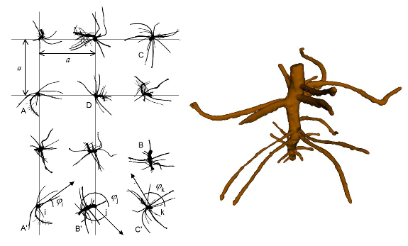
Figure 1: Projections onto a horizontal plane of the root systems of nine bean plants placed on a square lattice with spacing $a$ are shown in the first three rows of the left panel. The last row shows three root systems A’, B’ and C’ which are obtained by rotation about a vertical axis of randomly chosen plants A, B and C by random angles $\varphi_{i}$, $\varphi_{j}$ and $\varphi_{k}$, respectively. This row represents a typical pattern of the lattice model studied here. The right panel shows a 3 dimensional image of the root system D from the left panel.

The root systems thus obtained (see Fig. 1) were used as hosts in a lattice model to study the invasion of a soil-borne SIR epidemic spreading through a population of plants by mycelial growth from root system to root system. The lattice model was created in the following manner. An arbitrary root system (e.g. A in Fig. 1) was selected from the nine experimentally available systems (see first three rows in the left panel of Fig. 1). This root system was rotated by a random angle $0<\varphi<2\pi$ about a vertical axis passing through the original bean and then placed on a node (with the bean-seed position coinciding with the node) $i$ ($i=1,2,\ldots,L^{2}$) of a square lattice of size $L\times L$ with lattice spacing $a$ (e.g. root A’ in Fig. 1). This process was repeated for all the nodes of the lattice. Several realizations ($\sim 10^{3}$) of so created lattice systems form a statistical ensemble which has been analysed below.

A soil-borne epidemic can be modelled by introducing a pathogen, in the form of a small fungal colony typical of R. solani onto a root system near the centre of the lattice. The pathogen is assumed to infect the initial plant and to grow along and around the root system by mycelial extension exploring the soil nearby. If another root system is situated nearby, the fungal colony can reach it and eventually infect it. In this way, the fungal colony propagates through a population of roots.

The transmission rate between plants in the SIR process, which is effected by mycelial spread between root systems, is proportional to the effective overlap between different 3d root systems. In order to characterize this overlap quantitatively, we first define the root number density (number of voxels per volume) in the following way. The roots (comprising the primary root and first-order lateral roots) in our model are represented by 3d digital images. Each image, $i$, consists of a set of $N_{i}$ voxels (three-dimensional pixels) with volume $V_{\text{voxel}}=10^{-3}\,\text{mm}^{3}$, the locations of which are given by position vectors ${\bf{r}}_{ni}=(x_{ni},y_{ni},z_{ni})$ with $n=1,\ldots,N_{i}$. The root number density that the image represents, $\rho_{\text{scan},i}({\bf{r}})$, is equal to $1/V_{\text{voxel}}$ if ${\bf{r}}$ coincides with the position of one of the voxels and zero otherwise. On the scale of the system, the number density of voxels can be written as a sum of Dirac delta-functions,

$$\rho_{\text{scan},i}({\bf{r}})=\sum_{n=1}^{N_{i}}\delta({\bf{r}}-{\bf{r}}_{ni})~{}.$$ (4)

Bearing in mind that the density should describe some additional volume around each root across which the fungus can spread though soil, known as the pathozone (Gilligan, 1995), and which therefore mediates the transmission of infection from a donor (i.e. infected) to a recipient (susceptible) root system, we apply broadening to the images replacing the Dirac delta-functions in Eq. (4) (or voxels) by their Gaussian representation, i.e.

$$\rho_{i}({\bf{r}})\simeq\int\text{d}{\bf{r^{\prime}}}\rho_{\text{scan},i}({\bf{r^{\prime}}})\left({1\over{2\pi\sigma^{2}}}\right)^{3/2}\exp{\left[-{({\bf{r}}-{\bf{r^{\prime}}})^{2}\over{2\sigma^{2}}}\right]}~{},$$ (5)

with the broadening parameter $\sigma=1.5$  (the value of $\sigma$ is much smaller than the lattice spacing, i.e. $\sigma\ll a$, so that the overlap with next-nearest neighbours and thus transmission of the pathogen to them can be ignored in the model) of the linear size of the voxel (pixel) (the abbreviation px is used below for pixel). This mimics the diffusive spread of a pathogen into the medium surrounding the root (Gilligan, 1995).

The fungal colony can efficiently pass between different roots through the volume of soil if branches of both roots are present in that volume, i.e. if the roots overlap. Therefore, we assume that transmission between nearest-neighbour hosts $i$ and $j$ separated by unit cell vector takes place at a rate $\beta_{ij}$, proportional to the 3d overlap $J_{ij}$ between the two hosts, i.e

$$\beta_{ij}=kJ_{ij}~{},$$ (6)

where,

$$J_{ij} = V_{\text{voxel}}\int\text{d}{\bf{r}}\rho_{i}({\bf{r}})\rho_{j}({\bf{r}})$$ (7)

$$= V_{\text{voxel}}\sum_{m=1}^{N_{i}}\sum_{n=1}^{N_{j}}\left({1\over{4\pi\sigma^{2}}}\right)^{3/2}\exp{\left[-{({\bf{r}}_{mi}-{\bf{r}}_{nj})^{2}\over{4\sigma^{2}}}\right]}~{}~{}.$$

The value of $J_{ij}$ (dimensionless) is the number of voxels of root $i$ in the region of the overlap with root $j$. From the definition, $J_{ij}=J_{ji}$. The coefficient $k$, the infection efficiency, has the meaning of transmission rate per overlapping voxel and is set to be the same for all overlapping roots. This efficiency represents the ability of the pathogen to utilise a point of contact between two hosts to spread between them. It therefore takes into account all details of the transmission process not associated with the host morphology and specific to the particular host-pathogen system, such as susceptibility and infectivity, together with other factors such as environmental conditions that, in turn, influence transmission of infection. We therefore investigate the role of morphology in deciding the overall rate between two root systems, with all other properties decribed by variable values of $k$. Therefore, both the transmission rate, $\beta_{ij}$, between an arbitrary pair of the nearest-neighbour hosts and thus transmissibility,

$$T_{ij}=1-\exp\{-kJ_{ij}\}~{},$$ (8)

(see Eq. (1)), depend on the transmission efficiency $k$, being a control parameter, and the random overlap $J_{ij}$ which depends on distance between hosts $a$, being another control parameter. The randomness in the overlaps is caused by the complex morphology of hosts. With these assumptions, all the information about a given spatial configuration of the system (a particular realization of roots and angles at each node) is contained in the set of overlaps $\{J_{ij}\}$, while all the information about the epidemiological properties of the system is contained in the set of transmissibilities $\{T_{ij}\}$.

Typical probability densities $\rho(J_{ij})$ and $\rho(T_{ij})$ for the ensemble of roots are shown in Fig. 2 and Fig. 3. It follows from Fig. 2 that $\rho(J_{ij})$ is a monotonically decaying function. The value of $J$ roughly corresponds to the number of pixels in the overlap region. In the region of very small overlaps $J_{ij}\lesssim{1}$ (i.e. the overlap is either less than or of order of unity) caused by Gaussian broadening effects for pixels,

$$\rho(J_{ij})\propto J_{ij}^{-\alpha}~{},$$ (9)

with $\alpha\simeq 0.9$ (see the inset in Fig. 2). For the most interesting range of $1\lesssim{J}_{ij}\lesssim{1}0^{3}$, the probability density decays according to Eq. (9) with $\alpha\simeq 0.5$ (see Fig. 2). For larger values of $J_{ij}$ the function $\rho(J_{ij})$ exhibits even faster decay.

The shape of the probability density for transmissibilities follows from the mapping given by Eq.(8). The semi-infinite range of $J_{ij}$ is mapped onto a finite interval for transmissibilities, $0\leq T_{ij}\leq 1$, in such a way that all the large values of $J_{ij}$ are accumulated around $T_{ij}\simeq 1$ and all small values of $J_{ij}$ are concentrated around $T_{ij}\simeq 0$. As a consequence the monotonic distribution $\rho(J_{ij})$ gives rise to a distribution with two maxima (see Fig. 3)). The relative weights of the peaks depend upon the value of the transmission efficiency, $k$. For small values of $k\lesssim{k}_{c}$, the peak around zero is dominant (see the solid line in Fig. (3)) ensuring the non-active regime for epidemics, i.e. there is no invasion. In contrast, for large values of $k\gtrsim{k}_{c}$, the peak around unity becomes dominant for the distribution of transmissibilities and the SIR process is active (see the dot-dashed line in Fig. (3)). At criticality, $k=k_{c}$, the distribution of transmissibilities is approximately symmetric around $T=1/2$ (see the dashed line in Fig. (3)).

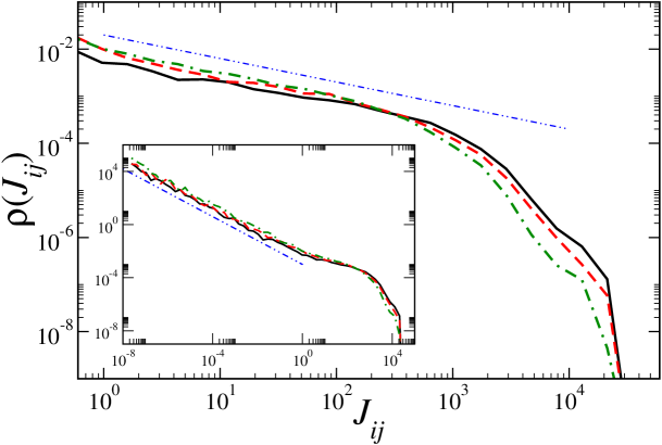
Figure 2: Probability density function $\rho(J_{ij})$ for overlaps, $J_{ij}$, between root systems in double-log scale for different lattice spacings: $a=100$ px^1/2 (solid curve), $a=120$ px^1/2 (dashed) and $a=150$ px^1/2 (dot-dashed). The double dot-dashed line corresponds to $\rho(J_{ij})\propto J_{ij}^{-\alpha}$ with $\alpha=1/2$ (guide for eye only). The inset shows the same distributions on a larger scale with the double dot-dashed line corresponding to $\rho(J_{ij})\propto J_{ij}^{-\alpha}$ with $\alpha=0.9$ (guide for eye only).

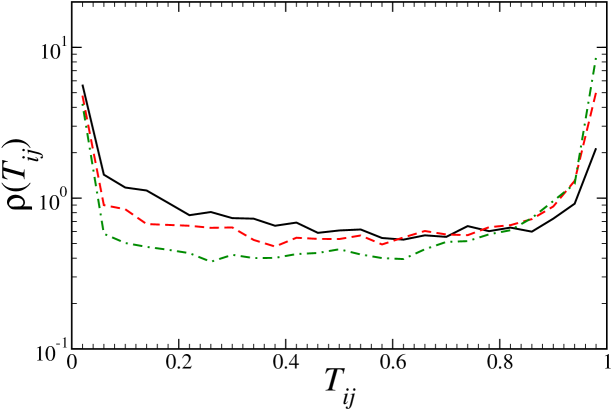
Figure 3: Probability density function $\rho(T_{ij})$ for transmissibilities, $T_{ij}$, in semi-log scale for three different values of the transmission efficiency, $k$: $k=k_{c}/2$ (solid curve), $k=k_{c}$ (dashed curve) and $k=2k_{c}$ with $k_{c}\simeq 0.00344$ for $a=120$ px^1/2.

3 Results

In this section, we present our main results on the behaviour of the SIR epidemic for the ensemble of realistic 3d root systems of bean plants placed on a regular lattice. We start with an evaluation of the invasion probability (order parameter) as a function of two control parameters, transmission efficiency and lattice spacing, paying special attention to the threshold values of the control parameters separating invasive and non-invasive regimes of epidemics. After that we compare the behaviour of the epidemic in our model with a mean-field system and find a significant role of correlations in transmissibilities of pairs of bonds separated by a relatively short distance. Finally, several “toy” models are investigated in order to clarify the effect of correlations.

3.1 Phase-diagram

One of the most important characteristics for epidemic spread is the probability of invasion. In the language of continuous phase transitions, the invasion probability, $P_{\text{inv}}$, is the order parameter defining the status of the epidemic to be either in the non-invasive ($P_{\text{inv}}=0$) or invasive ($P_{\text{inv}}>0$) regimes. In our model, the invasion probability depends on two control parameters, the transmission efficiency (specific to the host-pathogen system and independent of the spatial configuration) and the lattice spacing (affecting the set of overlaps $\{J_{ij}\}$), $P_{\text{inv}}=P_{\text{inv}}(k,a)$.

In order to calculate $P_{inv}(k,a)$ for a particular set of transmissibilities $\{T_{ij}\}$, we use the mapping to bond percolation and create many stochastic realizations in which each bond $i-j$ is occupied with probability $T_{ij}$. The probability of invasion is defined in an infinite system as the probability that any given site belongs to an infinite, or spanning, cluster of sites. A single such spanning cluster will always exist above the invasion threshold in an infinite system, and will never exist below it. Therefore the invasion probability is equal to the fraction of sites out of the whole system that belong to this cluster, when it exists, and zero otherwise. Since it is clear that there will not be an infinite cluster in a finite system (which is all we can model), we define a spanning cluster here as one which spans the lattice touching all four boundaries. Then for each stochastic realization of the bonds, we determine if the spanning cluster exists, and what fraction of the system it makes up, thus obtaining an estimate of $P_{\text{inv}}$ from that realization. The average of these estimates over all stochastic realizations gives the probability of invasion for the particular values of $\{T_{ij}\}$.

A different realization of the set $\{T_{ij}\}$ would produce a slightly different value of the invasion probability. Therefore we have averaged the invasion probability over different realizations of $\{T_{ij}\}$, to obtain the configurational average of the invasion probability $\langle P_{inv}(k,a)\rangle$. This value is representative because the invasion probability is a self-averaging quantity (Binder & Young, 1986) as we have checked numerically.

Figure 4: The dependence of the configurationally averaged invasion probability, $\langle P_{inv}(k,a)\rangle$, on the transmission efficiency, $k$ (log-scale), and lattice spacing, $a$. The averaging has been done over $1000$ configurations of root systems on 200$\times$200 lattice with open boundary conditions. The line in the $a-\log(k)$ plane represents the phase boundary for the invasive and non-invasive regimes of an SIR epidemic. The critical values of $k$ for given $a$ have been obtained by finite-size scaling collapse with relative error $<2\%$.

The results of numerical simulations for the average invasion probability, $\langle P_{inv}(k,a;L)\rangle$, for a finite size, $L\times L$, lattice are presented in Fig. 4, with $L=200$. As expected, for large values of lattice spacing and small transmission efficiency the system is unsuited to pathogen invasion. In contrast, small lattice spacings and high values of $k$ enhance the probability of invasion and hence of an epidemic.

The invasion probability surface $\langle P_{inv}(k,a;L)\rangle$ shown in Fig. 4 depends on the lattice size $L$. When the system size becomes very large, $L\to\infty$, the values of the probability of invasion tend to a certain limiting surface. The line of the critical points $a_{c}=a_{c}(k_{c})$ (the solid line in the horizontal plane in Fig. 4) separating non-invasive ($\lim_{L\to\infty}\langle P_{inv}(k,a|L)\rangle=0$) and invasive ($\lim_{L\to\infty}\langle P_{inv}(k,a|L)\rangle>0$) regimes is of particular importance because it allows the safe (non-invasive) parameter region to be identified.

The data points on the phase boundary $a_{c}=a_{c}(k_{c})$ were obtained by finite-size scaling collapse in the following way. The dependence of the order parameter on the system size around the critical point (e.g. $k_{c}$) for continuous phase transition is well established (Isichenko, 1992),

$$\langle P_{\text{inv}}(k,a;L)\rangle=L^{-\frac{\beta}{\nu}}\tilde{P}_{\text{inv}}((k-k_{c})L^{\frac{1}{\nu}})~{},$$ (10)

where $\tilde{P}_{\text{inv}}$ is the scaling function and $\beta$ and $\nu$ are the universal scaling exponents. The scaling function can be found by scaling collapse of $\langle P_{\text{inv}}(k,a;L)\rangle$ for several system sizes using $k_{c}$ and scaling exponents as fitting parameters (Heermann & Stauffer, 1980). Technically this is achieved by plotting $\langle P_{\text{inv}}(k,a;L)\rangle L^{\frac{\beta}{\nu}}$ versus $(k-k_{c})L^{\frac{1}{\nu}}$ for several values of $L$, and finding the values of $\nu$, $\beta$ and $k_{c}$ that lead to a collapse of all the curves for different $L$ to a single one, which corresponds to $\tilde{P}_{\text{inv}}$. Such a finite-size scaling analysis was applied to evaluate the critical values of $k_{c}$ for given lattice spacings and the results are shown by the line in the horizontal plane in Fig. 4. The scaling collapse also gives the values of the scaling exponents, $\beta=0.13\pm 0.008$ and $\nu=1.32\pm 0.05$, which coincide with those for the isotropic percolation universality class (Isichenko, 1992). We have also performed the scaling collapse for the susceptibility (Heermann & Stauffer, 1980) and found the expected values for the corresponding scaling exponents and the invasion threshold. Therefore, we have confirmed that the continuous phase transition for invasion probability in the system of roots (with short-range correlations discussed below), as expected, is similar to that in isotropic percolation, i.e. it belongs to the isotropic percolation universality class.

3.2 Correlations

The invasion probability presented in Fig. 4 for a heterogeneous lattice with transmissibilities $\{T_{ij}\}$ has been calculated numerically by estimating the mean fraction of sites belonging to the spanning cluster in the bond-percolation problem. Alternatively, we could use a mean-field assumption (Eq. (3)), which suggests that the heterogeneous system is equivalent to a homogeneous one with average transmissibility $\langle T\rangle$, if there are no correlations between transmissibilities. This would prove that the spread of the soil-borne pathogen in the root system is not be affected by the heterogeneity of the hosts. To test the validity of the mean-field approach for our model, in Fig. 5, we show the dependence of the invasion probability on mean transmissibility both for heterogeneous (solid curve) and homogeneous mean-field (dashed curve) systems. Evidently, the critical value of the transmissibility in the real-root system is greater than that in the mean-field system, and thus the real-root system with inherent heterogeneity in transmissibilities is less vulnerable to epidemic invasion as compared with the homogeneous system with the same MEAN transmissibility. This implies the presence of correlations in transmissibilities between hosts in the system (Sander et al., 2002; Pérez-Reche et al., 2010). Note that these correlations are of a different nature to spatial-temporal correlations in the density of infected/removed hosts observed during the propagation of disease. The short-range correlations in transmissibilities make an epidemic less likely in the heterogeneous system under consideration (solid curve in Fig. 5) than in a homogeneous mean-field system (dashed curve) for values of $P_{\text{inv}}\lesssim{0}.95$.

It should be noted that for relatively large values of the mean transmissibility (e.g. $\langle T\rangle\gtrsim{0}.62$ in Fig. 5), the invasion probability for heterogeneous system is higher than for homogeneous one. This is a consequence of negative correlations in transmission (cf. Fig. 5). This behaviour is in contrast with that for systems with non-negative correlations in transmission such as, e.g. a system with heterogeneous recovery times. Indeed, in this case it can be rigorously shown that the probability of invasion in a homogeneous system cannot be smaller than that for heterogeneous systems for any value of $\langle T\rangle$ (Kuulasmaa, 1982; Cox & Durrett, 1988; Kenah & Robins, 2007; Miller, 2007). However, this theorem does not apply to systems with negative correlations, such as the root system studied here.

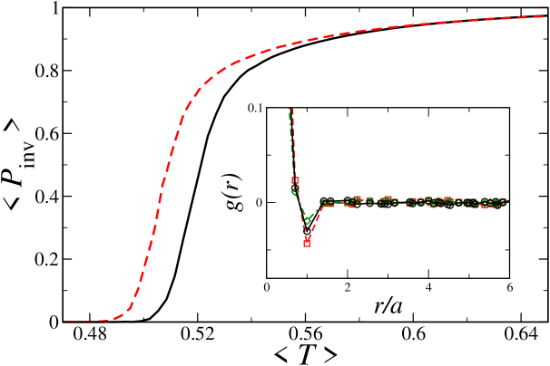
Figure 5: Invasion probability $P_{\text{inv}}$ versus mean transmissibility $\langle T\rangle$ for the realistically complex roots systems in which transmissibilities between two hosts are calculated according to Eq. (8) (the solid curve) and the mean-field system in which all the transmissibilities coincide with the mean transmissibility $\langle T\rangle$ (the dashed curve). The lattice spacing is $a=120$ px^1/2 and values of all other parameters are the same as those used in Fig. 4. The inset shows the spatial correlation function, $g(r)$, for transmissibilities evaluated at critical transmission efficiency, $k_{c}(a=120)\simeq 0.00344$ (circles connected by solid line), $k=k_{c}/2$ (squares connected by the dashed line) and $k=2k_{c}$ (diamonds connected by the dot-dashed line).

The difference in the invasion curves for heterogeneous and homogeneous systems (cf. solid and dashed curves in Fig. 5) is a clear indication of the correlations in transmissibilities for heterogeneous systems. Indeed, the spatial correlation function for transmissibilities,

$$g(r)=\frac{\langle T_{ij}T_{km}\rangle-\langle T_{ij}\rangle\langle T_{km}\rangle}{\langle T_{ij}\rangle\langle T_{km}\rangle}=\frac{\langle T_{ij}T_{km}\rangle}{\langle T\rangle^{2}}-1~{},$$ (11)

plotted in the inset to Fig. 5, shows the presence of negative short-range (between nearest bonds) correlations (see the dip at $r/a=1$ in the inset of Fig. 5). In Eq. (11), the distance $r$ is taken between midpoints of different bonds $i-j$ and $k-m$ and the averaging is performed over all bond pairs separated by the same distance.

Therefore, the SIR process in the system of real roots can be mapped onto the bond-percolation problem with short-range correlations between bond probabilities. In the next subsection, we reveal the origin of such correlations.

3.3 Disc-Based Models

In order to understand the origin of the short-range correlations in transmissibilities between roots, we study three simplified “toy” models of differing complexity. In all these models, each root system $i$ is replaced by a two-dimensional horizontal “disc”, i.e. by the number density $\rho_{i}({{\bf{r}}})$ with the centre of mass at ${{\bf{r}}}_{i}$. The centres of the discs are randomly displaced from the lattice nodes characterized by position vectors ${{\bf{r}}}_{i}^{(0)}$, i.e. ${{\bf{r}}}_{i}={{\bf{r}}}_{i}^{(0)}+\Delta{{\bf{r}}}_{i}$, where the displacement vectors are normally distributed, $\Delta{{\bf{r}}}_{i}\sim N_{2}(0,\sigma^{2}_{\Delta})$, with zero expectation value and variance, $\sigma^{2}_{\Delta}$. This normal distribution of $\Delta{{\bf{r}}}_{i}$ mimics the anisotropy in the shape of real root systems, i.e. the fact that the centres of mass of roots are displaced with respect to the seed (node) positions. The toy models then differ amongst each other by the form of the function used for $\rho_{i}({{\bf{r}}})$ and therefore by the value of overlaps between two discs.

In the first model (see Fig. 6(a)), all the discs have the same radius, $R$, and constant number density, $\rho_{i}({{\bf{r}}})=\rho_{0}$ if $|{{\bf{r}}}-{{\bf{r}}}_{i}|\leq R$, and zero density otherwise. The overlap between two discs $i$ and $j$ with centres separated by distance $d_{ij}=|{{\bf{r}}}_{j}-{{\bf{r}}}_{i}|$ reads

$$J^{(1)}_{ij}=V_{\text{pixel}}\int\text{d}{{\bf{r}}}\rho_{i}({{\bf{r}}})\rho_{j}({{\bf{r}}})=2\rho_{0}^{2}R^{2}\left[\cos^{-1}(d_{ij}/2R)-(d_{ij}/2R)\sqrt{1-(d_{ij}/2R)^{2}}\right]~{},$$ (12)

if $d_{ij}/2R\leq 1$ and zero otherwise (with the pixel area $V_{\text{pixel}}=1$). This is one of the simplest models, which is equivalent to a representation of the real root systems by identical uniform vertical cylinders projected onto the horizontal plane.

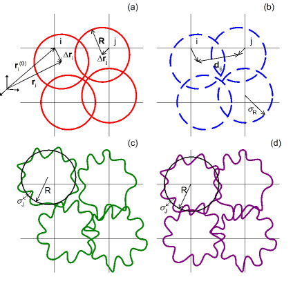
Figure 6: Disc-based toy models: (a) displaced solid discs; (b) displaced dispersed discs; (c) displaced discs with irregular edges (d) non-displaced discs with irregular edges

In the second model (see Fig. 6(b)), the density is normally distributed around ${{\bf{r}}}_{i}$ with variance $\sigma^{2}_{R}$, i.e.

$$\rho_{i}({{\bf{r}}})=\tilde{\rho}(2\pi\sigma_{R}^{2})^{-1}\exp{\left(-|{{\bf{r}}}-{{\bf{r}}}_{i}|^{2}/2\sigma_{R}^{2}\right)}~{},$$

where $\tilde{\rho}$ is a dimensionless normalization constant, and the overlap between two dispersed discs represented by Gaussian functions is

$$J^{(2)}_{ij}=\frac{{\tilde{\rho}}^{2}}{4\pi\sigma_{R}^{2}}\exp{\left(-d_{ij}^{2}/4\sigma_{R}^{2}\right)}~{}.$$ (13)

The second model accounts for the property that the number density in real roots is a decaying function with distance from the main tap root.

The third model (see Fig. 6(c)) mimics the angular irregularity in the shape of real root systems, i.e. the fact that overlap significantly depends on the angle $\varphi$ at which the roots are placed at the lattice nodes (see Fig. 1). In this model, we assume that the overlap has two contributions,

$$J^{(3)}_{ij}=J^{(1)}_{ij}+\delta J_{ij}~{},$$ (14)

where $J^{(1)}_{ij}$ is given by Eq. (12) as in the first model and a random normally distributed constituent, $\delta J_{ij}\sim N(0,\sigma_{J}^{2})$, with the variance, $\sigma_{J}^{2}$, which can depend on $J^{(1)}_{ij}$.

In order to illustrate that irregularity in shape alone is insufficient to cause the observed effect, we concider a fourth model, which is a special case of the third model, where there is no displacment of the discs (i.e. we set $\sigma^{2}_{\Delta}=0$). Here we see no correlations (see the dot-double dashed line with left triangles in the inset in Fig. 7), and thus the system can be approximated by an equivilent homogeneous system (the dot-double dashed line with left triangles coincides with the solid line marked by crosses in in Fig. 7).

The disc-based models depend on several parameters, such as $R$, $\sigma^{2}_{\Delta}$, $\sigma^{2}_{R}$ and $\sigma^{2}_{J}$. The two normalization constants $\rho_{0}$ and $\tilde{\rho}$ can be incorporated into the value of the infection efficiency $k$ and are set, for convenience, to $\rho_{0}=\tilde{\rho}=1$. The values of the disc radius, $R$, in the first model and the width of the Gaussians in the second model, $\sigma_{R}$, can be estimated from the mean value (amongst all $N_{r}$ roots) of the variance of the real root density projected onto the horizontal plane, i.e.

$$R^{2}=\sigma^{2}_{R}=N_{r}^{-1}\sum_{i}^{N_{r}}\delta{{\bf{r}}}_{\perp i}^{2}~{},$$ (15)

where

$$\delta{{\bf{r}}}_{\perp i}^{2}=\int\text{d}{{\bf{r}}}({{\bf{r}}}-{{\bf{r}}}_{i})_{\perp}^{2}\rho_{i}({{\bf{r}}})~{},~{}~{}~{}\text{and}~{}~{}~{}{{\bf{r}}}_{i}=\int\text{d}{{\bf{r}}}({{\bf{r}}}-{{\bf{r}}}_{i}^{(0)})\rho_{i}({{\bf{r}}})~{},$$ (16)

with $\rho_{i}({{\bf{r}}})$ given by Eq. (5) and suffix $\perp$ referring to the vector component perpendicular to the vertical axis. This value is found to be $R=\sigma_{R}\simeq 73$ px^1/2. Similarly, the value of $\sigma^{2}_{\Delta}$ was estimated as

$$\sigma^{2}_{\Delta}=N_{r}^{-1}\sum_{i}^{N_{r}}({{\bf{r}}}_{i}-{{\bf{r}}}_{i}^{(0)})^{2}\simeq 1444\text{px}~{},$$ (17)

The value of $\sigma^{2}_{J}$ can be estimated from the variance of the overlap $J_{ij}(\varphi_{i},\varphi_{j})$ between two real roots which stochastically depends on their orientations characterized by $\varphi_{i}$ and $\varphi_{j}$ (see Fig. 1), and it is found to be $\sigma_{J}/\langle J^{(1)}_{ij}\rangle\simeq 1.35$.

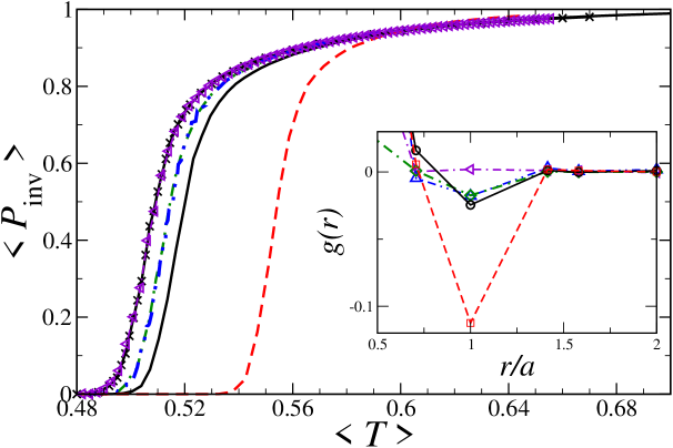
Figure 7: The invasion curves for mean-field system (solid curve marked by the crosses), which coincides exactly with that for the non-displaced irregular discs model (dot-double dashed with triangles), real-root system (solid), solid-disc model (dashed), dispersed disc model (dot-dashed) and discs with irregular edges (double dot-dashed). The inset shows the correlation functions in the region around the negative dip (the same curve styles are used).

Having the estimates of all the parameters for the toy models it is straightforward to evaluate numerically the dependence of the invasion probability on mean transmissibility. The results presented in Fig. 7 clearly demonstrate that, for all the models exhibiting anisotropy, the critical point $T_{c}$ is shifted to the right of that for the mean field system and the invasion probability is also reduced in a rather wide range, $0\leq P_{\text{inv}}\lesssim{0}.95$, as compared with the homogeneous system (note, that models 2 and 3 reproduce the real root system reasonably well). This is a consequence of the short-range correlations in transmissibilities present in the disc-based models. The bigger shift for the first model as compared with less significant shifts for models 2 and 3 reflects the respective decrease in the scale of correlations for the latter models (cf. dashed, dot-dashed and double dot-dashed curves in Fig. 7 and corresponding curves in the inset). The relatively large correlations in the first model are due to sharp disc boundaries so that the overlaps are significantly larger (smaller) for spatially close (distant) discs as compared with the mean value. This difference is diminished by the Gaussian broadening of the disc density so that the correlations for the second model are less pronounced. The angular fluctuations of density (model 3) result in a similar reduction of correlations found for the solid disc model.

We conclude from the analysis of the toy models that anisotropy in the root shape accounts for most of the short-range correlations in transmissibilities between the root systems. Anisotropy arises mainly from the horizontal shift of the centre of mass with respect to the lattice node (seed) location. To the greatest extent, this effect is picked up by the first model which displays the most significant effect of correlations. Dispersion and irregularity in the root shapes mimicked by models 2 and 3, respectively, reduce the level of correlations. Finally, if irregular discs are not displaced from the lattice nodes (model 4) the correlations completely disappear and the model is equivalent to the mean-field one.

4 Discussion

The occurrence of well-defined phase transitions in determining whether or not a pathogen invades through a lattice of homogeneous hosts is well established (Grassberger, 1983). Following initial work by Bailey et al. (2000) on the spread of the soil-borne fungus, R. solani, critical percolation phenomena and phase transitions in lattice-based systems have been supported by experimental analysis. More recently, the concept has been extended to the transmission of soil-borne infections through lattices with missing sites (Otten et al., 2004) and through animal populations, exemplified by the spread of plague through gerbil populations in lattices of interconnecting burrows (Davis et al., 2008). Here we have extended the theoretical analysis of critical percolation phenomena to take account of the spatial correlations that occur in the set of morphologically complex 3d hosts represented by plant root systems.

We have used digitized images of the root systems of bean seedlings to provide realistic examples of a complex morphological branching structure to test the methodology. However, our results and methodological approaches, in particular the new disc-based models, provide a basis for further analysis of the transmission of infection and disease through a broad range of morphological structures.

We have shown that the invasion probability $(P_{inv})$ of a root-infecting pathogen spreading through a population of plants with morphologically-complex, overlapping 3d root systems, depends upon the transmissibility of infection between neighbouring plants (Eq. (1)). We have resolved the transmission into two components, the transmission efficiency $(k)$ between nearest neighbours, and the lattice spacing between plants $(a)$, which control the degree of overlap. The transmission efficiency is a measure of the probability of infection arising from overlap between an infected and a susceptible root system. Here we assume a constant transmission rate per overlapping voxel for overlapping roots but this assumption could be relaxed. The extent of the overlap is broadened to allow for the ability of the pathogen to explore soil immediately surrounding a root, known as the pathozone (Gilligan, 1983). The spacing between plants controls the degree of overlap. We have used the mapping to bond percolation in order to calculate the invasion probability for a set of transmissibilities, showing evidence for a marked phase transition that depends upon $k$ and $a$ (Fig. 4). We conclude that the heterogeneities in transmissibilities arising from correlations in degree of overlap between neighbouring plants, renders a population of root systems more less vulnerable to epidemic invasion than a corresponding uncorrelated homogeneous system.

For concreteness, we have analyzed the square-lattice topology only. Any other regular lattice topologies can be treated in a similar way. The invasion curve, $P_{\text{inv}}(\langle T\rangle)$, is specific for the lattice topology but the effect of correlations in transmissibilities between root systems will be qualitatively the same as that found for the square lattice. In modelling the spread of an SIR epidemic through heterogeneous, overlapping root systems, we have used several simplifications. One of these is related to the assumption of identical recovery times for all the hosts. If this assumption is relaxed and the recovery times are distributed according to a certain probability density function then the invasion probability in such a system is lower than that in the system with homogeneous recovery times (Kuulasmaa, 1982; Cox & Durrett, 1988). We have demonstrated this using several realistic distributions for recovery times in root systems. The results presented in Fig. 8 clearly show a shift of invasion curves to the right, thus indicating that systems with heterogeneity in recovery times are indeed more resistant to SIR epidemics. The main reason for such increased resistance is that the heterogeneity in recovery times brings positive correlations to the system (see inset in Fig. 8 and  Kuulasmaa (1982); Cox & Durrett (1988); Miller (2007); Kenah & Robins (2007)).

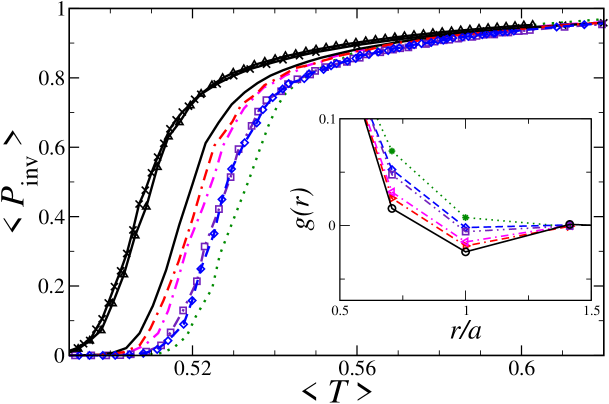
Figure 8: The invasion curves for the mean-field system (solid curve marked by the crosses), the real-root system with homogeneous recovery times (solid), and distributed with $\text{log}(\tau)\sim N(0,0.5)$ (dot double-dashed), $\text{log}(\tau)\sim N(0,1)$ (dashed with diamonds), $\tau\sim N(1,0.5)$ (dot-dashed), $\tau\sim N(1,1)$ (double dot-dashed with squares), $\tau\sim\text{Exponential}(1)$ (dotted). The solid line marked by triangles represents an anisotropic system of identical roots in identical orientation. The inset shows the correlation functions (the same curve styles are used).

Another assumption in our approach is that the root anisotropy is in a random direction for each root. However, in a real planting, large scale resource gradients can lead to a predominant orientation of all root systems. This results in anisotropy of the overlaps $J_{ij}$ meaning that the root overlaps along a certain direction are greater than those in other directions. In fact, the system becomes more ordered typically exhibiting larger transmissibilities in the direction of resource gradients. For illustration, we considered an extreme case for which an epidemic spreads through a system of anisotropically identical roots placed in the same orientation (without rotation) on all the nodes of a square lattice. The results are presented by the solid curve marked by triangles in Fig. 8 from which it follows that the system of identical anisotropic roots is more vulnerable than the system of randomly rotated roots (cf. the dashed curve with the solid one) meaning that the external gradients may reduce the resilience of the system. This is an expected effect because the SIR epidemic in the system of identical anisotropic roots can be mapped onto anisotropic percolation characterized by two transmissibilities $T_{x}\neq T_{y}$ along different lattice directions. It is known (Sykes & Essam, 1964), that the invasion threshold in such a system coincides with that in homogeneous one, i.e. given by the following equation, $T_{c}=\langle T\rangle=(T_{x}+T_{y})/2=1/2$ (for square lattice), which can be seen from Fig. 8 (cf. solid lines marked by triangles and crosses).

In the analysis above we have used the toy models in order to understand the spread of epidemics in systems of morphologically realistic roots. The models were designed in such a way as to capture the main features of root systems that influence the spread of epidemics. Our analysis of the toy models reveals that anisotropy, rather than disorder in root shape, has the major effect on epidemic invasion. The anisotropy in the real root systems is due to the fact that the 3d root density distribution is not centrally located beneath the seed. By mimicking a similar effect within toy models, we find that the greater the degree of root anisotropy, the more resistant the system is to epidemic invasion. The effect is due to anisotropy-induced, short-range correlations in disease transmissibilities between different root systems which result in a reduced probability of invasion. These correlations are such that a root system that is well connected with one of its neighbours is likely to be poorly connected with its neighbour on the opposite side.

The other root characteristic, morphological complexity, has an opposite effect on the probability of epidemic invasion. By morphological complexity, we mean that the roots branch producing secondary roots so that the shape of the root system becomes irregular. The increase in degree of branching makes the system more isotropic and diminishes the correlation effects thus enhancing the vulnerability of the system to epidemics. This has been demonstrated with toy models by introducing disorder, characterised by the parameter $\sigma_{J}$ mimicking the degree of branching. Overall we can conclude that highly anisotropic and poorly branching root systems render the population less prevalent to invasion of soil-borne pathogens.

In our analysis, we have used the roots of young bean seedlings, grown under hydroponic conditions. These serve to illustrate the methodology. The hydroponically grown bean roots exhibit an inherent anisotropy in their shapes which is the main morphological factor in reducing the invasion probability. Further work will consider the root morphology of monocotyledenous as well as dicotyledenous root systems grown and imaged in soil. We also assume quenched disorder in the systems considered here. This means that all the properties of the hosts, including their morphology, do not depend on time. Such an assumption is true only in the case of relatively fast epidemics and/or slowly growing root systems. Of course, in real situations, the root morphology can significantly change in the course of an epidemic requiring time-dependent transmissibilities, that are beyond the scope of this paper but comprise an important topic for further study.

5 Acknowledgments

TPH would like to thank the UK EPSRC for financial support. FJPR, SNT, FMN and CAG thank BBSRC for funding (Grant No. BB/E017312/1). Luciano da F. Costa thanks CNPq (301303/2006-1 and 573583/2008-0) and FAPESP (05/00587-5) for sponsorship. Mauro Miazaki thanks FAPESP (07/50988-1) for his grant and Christopher Gilligan gratefully acknowledges the support of a BBSRC Professorial Fellowship. The authors thank Alexandre Cristino for suggestions regarding the growth of the seeds.

References

- Bailey et al. (2000) Bailey, D., Otten, W. & Gilligan, C. A. 2000 Saprotrophic invasion by the soil-borne fungal plant pathogen Rhizoctonia solani and percolation thresholds. New Phytologist, 146(3), 535–544.
- Binder & Young (1986) Binder, K. & Young, A. P. 1986 Spin glasses: Experimental facts, theoretical concepts, and open questions. Rev. Mod. Phys., 58, 801.
- Cox & Durrett (1988) Cox, J. & Durrett, R. 1988 Limit theorems for the spread of epidemics and forest fires. Stoch. Proc. Appl., 30, 171–191.
- Davis et al. (2008) Davis, S., Trapman, P., Leirs, H., Begon, M. & Heesterbeek, J. A. P. 2008 The abundance threshold for plague as a critical percolation phenomenon. Nature, 454, 634–637.
- Diekmann & Heesterbeek (2000) Diekmann, O. & Heesterbeek, J. 2000 Mathematical epidemiology of infectious diseases: model building, analysis and interpretation. Wiley.
- Dybiec et al. (2004) Dybiec, B., Kleczkowski, A. & Gilligan, C. A. 2004 Controlling disease spread on networks with incomplete knowledge. Phys. Rev. E, 70, 066 145.
- Gilligan (1983) Gilligan, C. A. 1983 Modeling of soilborne plant pathogens. Annual Review of Phytopathology, 21, 45–64.
- Gilligan (1990) Gilligan, C. A. 1990 Mathematical modelling and analysis of soilborne pathogens. In Epidemics of plant diseases (ed. J. Kranz), pp. 96–142. Heidelberg: Springer.
- Gilligan (1995) Gilligan, C. A. 1995 Modelling soil-borne plant pathogens: reaction-diffusion models. Canadian Journal of Plant Pathology, 17, 96–108.
- Gilligan (2002) Gilligan, C. A. 2002 An epidemiological framework for disease management. Advances in Botanical Research, 38, 1–64.
- Gilligan et al. (1994) Gilligan, C. A., Brassett, P. R. & Campbell, A. 1994 Modeling of early infection of cereal roots by the take-all fungus - a detailed mechanistic simulator. New Phytologist, 128(3), 515–537.
- Grassberger (1983) Grassberger, P. 1983 On the critical behavior of the general epidemic process and dynamical percolation. Math. Biosc., 63, 157–172.
- Heermann & Stauffer (1980) Heermann, D. W. & Stauffer, D. 1980 Influence of Boundary conditions on square bond percolation near . Z Physik B - Condensed Matter, 40, 133–136.
- Hinrichsen (2000) Hinrichsen, H. 2000 Non-equilibrium critical phenomena and phase transitions into absorbing states. Adv. Phys., 49, 815.
- Hornby (1990) Hornby, D. 1990 Biological control of soil-borne plant pathogens. Wallingford, UK: CAB International.
- Isichenko (1992) Isichenko, M. B. 1992 Percolation, statistical topography, and transport in random media. Rev. Mod. Phys., 64, 961–1043.
- Jackson (2008) Jackson, M. 2008 Social and economic networks. Princeton University Press.
- Keeling & Rohani (2007) Keeling, M. J. & Rohani, P. 2007 Modeling infectious diseases in humans and animals. Princeton University Press.
- Kenah & Robins (2007) Kenah, E. & Robins, J. M. 2007 Second look at the spread of epidemics on networks. Phys. Rev. E, 76, 036 113.
- Kuulasmaa (1982) Kuulasmaa, K. 1982 The spatial general epidemic and locality dependent random graphs. J. Appl. Prob., 19, 745–758.
- Liggett (1985) Liggett, T. M. 1985 Interacting particle systems. New York: Springer-Verlag.
- Marro & Dickman (1999) Marro, J. & Dickman, R. 1999 Nonequilibrium phase transitions in lattice models. Cambridge: Cambridge University Press.
- Miller (2007) Miller, J. C. 2007 Epidemic size and probability in populations with heterogeneous infectivity and susceptibility. Phys. Rev. E, 76(1), 010 101. (doi:10.1103/PhysRevE.76.010101)
- Murray (2002) Murray, J. D. 2002 Mathematical Biology. I. An Introduction. Springer, 3rd edn.
- Nâsell (2002) Nâsell, I. 2002 Stochastic models of some endemic infections. Math. Biosci., 179, 1 – 19. (doi:DOI: 10.1016/S0025-5564(02)00098-6)
- Newman (2002) Newman, M. 2002 The spread of epidemic disease on networks. Phys. Rev. E, 66, 016 128.
- Ódor (2004) Ódor, G. 2004 Universality classes in nonequilibrium lattice systems. Rev. Mod. Phys., 76, 663.
- Otten et al. (2004) Otten, W. Bailey, D. & Gilligan, C. A. 2004 Empirical evidence of spatial thresholds to control invasion of fungal parasites and saproptrophs. New Phytologist, 163(1), 125–132.
- Pastor-Satorras & Vespignani (2003) Pastor-Satorras, R. & Vespignani, A. 2003 In Handbook of graphs and networks: From the genome to the internet (eds S. Bornholdt & H. G. Schuster). Berlin: Wiley-VCH.
- Pastor-Satorras & Vespignani (2004) Pastor-Satorras, R. & Vespignani, A. 2004 Evolution and structure of the internet: A statistical physics approach cambridge. Cambridge: Cambridge University Press.
- Pérez-Reche et al. (2010) Pérez-Reche, F. J., Taraskin, S. N., da F. Costa, L., Neri, F. M. & Gilligan, C. A. 2010 Complexity and anisotropy in host morphology make populations less susceptible to epidemic outbreak. To be published in J. R. Soc. Interface.
- Sander et al. (2002) Sander, L., Warren, C. P., Sokolov, I. M., Simon, C. & Koopman, J. 2002 Percolation on heterogeneous networks as a model for epidemics. Math. Biosc., 180, 293–305.
- Stauffer & Aharony (1992) Stauffer, D. & Aharony, A. 1992 Introduction to percolation theory. London: Taylor and Francis, 2nd edn.
- Sykes & Essam (1964) Sykes, M. F. & Essam, J. W. 1964 Exact critical percolation probabilities for site and bond problems in two dimensions. J. Math. Phys., 5, 1117–1127.