Abundance determination from global emission-line SDSS spectra: exploring objects with high N/O ratios

Abstract

We have compared the oxygen and nitrogen abundances derived from global emission-line SDSS spectra of galaxies using (1) the $T_{e}$ method and (2) two recent strong line calibrations: the ON and NS calibrations. Using the $T_{e}$ method, anomously high N/O abundances ratios have been found in some SDSS galaxies. To investigate this, we have Monte Carlo simulated the global spectra of composite nebulae by a mix of spectra of individual components, based on spectra of well-studied H ii regions in nearby galaxies. We found that the $T_{e}$ method results in an underestimated oxygen abundance (and hence in an overestimated nitrogen-to-oxygen ratio) if H ii regions with different physical properties contribute to the global spectrum of composite nebulae. This effect is somewhat similar to the small-scale temperature fluctuations in H ii regions discussed by Peimbert. Our work thus suggests that the high $T_{e}$-based N/O abundances ratios found in SDSS galaxies may not be real. However, such an effect is not expected to be present in dwarf galaxies since they have generally an uniform chemical composition. The ON and NS calibrations give O and N abundances in composite nebulae which agree with the mean luminosity-weighted abundances of their components to within $\sim$0.2 dex.

1 Introduction

Metallicities play a key role in many studies of galaxies. Gas-phase oxygen and nitrogen abundances are broadly used to estimate these metallicities. It is believed (e.g. Stasińska, 2006) that emission lines in spectra of H ii regions are the most powerful indicators of the chemical composition of galaxies, both in the low- and intermediate-redshift universe. The spectra of a large number of individual H ii regions in nearby spiral and irregular galaxies have now been obtained (McCall, Rybski & Shields, 1985; Zaritsky, Kennicutt & Huchra, 1994; van Zee et al., 1998; van Zee & Haynes, 2006; Bresolin, Kennicutt, & Garnett, 1999; Bresolin et al., 2005, 2009, among many others). These spectroscopic measurements provide basis for investigations of metallicity properties (such as radial abundance gradients, central metallicities, etc) of galaxies (Zaritsky, Kennicutt & Huchra, 1994; van Zee et al., 1998; Bresolin, Kennicutt, & Garnett, 1999; Pilyugin, Vílchez, & Contini, 2004b, among others).

Kennicutt (1992) pioneered another method of spectral investigation of galaxies, considering the global, i.e. spatially unresolved, spectrophotometry of a sample of 90 galaxies spanning the entire Hubble sequence. In recent years, the number of available spectra of emission-line nebulae has increased dramatically due to the completion of several large spectral surveys such as the Sloan Digital Sky Survey (SDSS, York et al., 2000). Measurements of emission lines in SDSS spectra have been used for abundance determinations in a number of studies (Kniazev et al., 2004; Izotov et al., 2006; Tremonti et al., 2004; Asari et al., 2007; Thuan et al., 2010, among others). The auroral lines are measurable in a relatively large number of SDSS galaxies (Kniazev et al., 2004; Izotov et al., 2006) that provide the possibility to obtain $T_{e}$-based abundances for SDSS galaxies.

The SDSS spectra are obtained through 3-arcsec diameter fibers. At a redshift of $z=0.025$, the projected aperture diameter is $\sim$ 1.5 kpc, while it is $\sim$ 10 kpc at a redshift of $z=0.17$. This suggests that SDSS spectra of distant galaxies are closer to global spectra of galaxies, i.e. they are the integrated spectra of multiple rather than just one H ii region. Therefore the meaning of $T_{e}$-based abundances in SDSS galaxies is unclear. If a single giant H ii region, excited by a single star cluster, is responsible for the global SDSS spectrum then one can expect that the $T_{e}$-based abundance to be a good estimate of the true one. Such a situation occurs only in nearby SDSS galaxies and in some distant SDSS galaxies where a single supergiant H ii region, resulting from a strong starburst, makes a dominant contribution to the global spectrum. One can expect, however, that in a majority of distant SDSS galaxies, multiple individual H ii regions contribute to the global spectrum.

Ercolano et al. (2007, 2010) have investigated the effect of multiple ionization sources in H ii regions on the total elemental abundances derived from the analysis of collisionally excited emission lines. They considered the case of an ionizing set composed of two stellar populations with masses of 37 $M_{\sun}$ and 56 $M_{\sun}$. They have shown that the temperature structures of models with centrally concentrated ionizing sources can be quite different from those of models where the ionizing sources are randomly distributed within the volume, with generally non-overlapping Strömgren spheres. Since the SDSS composite nebula can be ionised by sources of different temperatures then the meaning of the measured electron temperature in distant SDSS galaxies and consequently, that of the $T_{e}$-based abundance is not evident.

This problem is in some sense similar to the one concerning the validity of the $T_{e}$-based abundances in H ii regions with small-scale temperature fluctuations (Peimbert, 1967) or/and with large variations of the electron temperature across the nebula (Stasińska, 1978, 2005). According to Peimbert, since the line fluxes in the spectrum of such a nebula are weighted in favor of the hot regions, the electron temperature estimated from the auroral-to-nebular lines ratio will be overestimated and the abundance underestimated. While the existence of such temperature fluctuations in individual H ii regions is still debated, temperature variations of individual H ii regions within a composite nebula are to be perfectly natural. Thus, such an effect is probably at work in the distant SDSS galaxies.

When the electron temperature of an extragalactic H ii region cannot be measured, then its location in some emission-line diagrams is used for estimating its oxygen abundance. This approach to abundance determination in H ii regions, proposed by Pagel et al. (1979) and Alloin et al. (1979), is usually referred to as the “strong line method”. Numerous relations have been proposed to convert metallicity-sensitive emission-line ratios into metallicity or temperature estimates (e.g. Dopita & Evans, 1986; Zaritsky, Kennicutt & Huchra, 1994; Vilchez & Esteban, 1996; Pilyugin, 2000, 2001; Denicolo, Terlevich & Terlevich, 2002; Pettini & Pagel, 2004; Tremonti et al., 2004; Pilyugin & Thuan, 2005; Liang et al., 2006; Stasińska, 2006; Bresolin, 2007; Pérez-Montero & Contini, 2009; Thuan et al., 2010). Although SDSS spectra of distant galaxies are closer to global galaxy spectra than to spectra of individual H ii regions, abundances in distant SDSS galaxies have been estimated using the strong line methods developed for abundance determination in individual H ii regions (Tremonti et al., 2004; Erb et al., 2006; Asari et al., 2007; Thuan et al., 2010, among others). This, despite the warning of Stasińska (2010) that the strong line methods should be used only for nebulae having the same structural properties as those of the calibration samples.

However, there is a reason to expect the calibrations may provide more robust abundances in composite nebulae than the $T_{e}$ method. For definiteness, we will discuss the case of oxygen abundances. The auroral and nebular lines originate in transitions from levels that differ significantly in energy, with the levels that give rise to the auroral line being at higher energies than those for nebular lines. Therefore, the emissivity of the auroral line depends much more strongly on the electron temperature in the nebula than that of the nebular line. Hence, the auroral and nebular line fluxes in the integrated spectra of composite nebulae are weighted in different ways: the hot regions will give relatively more weight to the auroral line than to the nebular lines. This means the nebular and auroral lines in the spectra of composite nebulae correspond to different temperatures, i.e. they are not self-consistent. The electron temperature estimated from the auroral-to-nebular lines ratio will then be overestimated and the abundance will be underestimated (Peimbert, 1967; Stasińska, 1978, 2005). In the case of the empirical calibrations considered here (the ON and NS calibrations), combinations of strong lines for different ions serve as abundance and electron temperature indicators. The differences between the energies of parent levels for these nebular lines are smaller than those between the energies of parent levels for the auroral and nebular lines. Then one can expect that, in the strong line method, the different regions will give roughly similar relative contributions to the nebular line fluxes, i.e. they will all correspond to more or less similar electron temperatures. This, in turn, will result in more robust global abundances estimates.

The goal of the present study is to examine to what extent abundances for distant SDSS galaxies derived in different ways (by the classic $T_{e}$ method and through recent calibrations) agree or disagree. The abundances of a sample of SDSS galaxies are examined in Section 2. In Section 3, we compare the data with artificial global spectra of composite nebulae generated by Monte Carlo techniques as mixes of spectra of individual components, using spectra of real H ii regions in nearby galaxies with measured electron temperatures. The meaning of abundances derived in composite nebulae in different ways and their locations in the O/H – N/O diagram are examined. A discussion of the results is given in Section 4. Section 5 presents the conclusions.

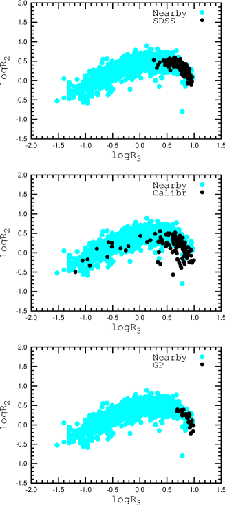
Figure 1: The log$R_{3}$ – log$R_{2}$ diagram. The filled dark (black in the color version) circles show the objects from our SDSS sample (upper panel), the sample of calibration H ii regions (middle panel), and the Green Pea galaxies (lower panel). The filled grey (light-blue in the color version) circles in each panel are objects from the sample of H ii regions in nearby galaxies. (A color version of this figure is available in the online version.)

Throughout the paper, we will be using the following standard notations for the line intensities:
$R$ = $I_{[OIII]\lambda 4363}/I_{{\rm H}\beta}$,
$R_{2}$ = $I_{[OII]\lambda 3727+\lambda 3729}/I_{{\rm H}\beta}$,
$N_{2}$ = $I_{[NII]\lambda 6548+\lambda 6584}/I_{{\rm H}\beta}$,
$S_{2}$ = $I_{[SII]\lambda 6717+\lambda 6731}/I_{{\rm H}\beta}$,
$R_{3}$ = $I_{{\rm[OIII]}\lambda 4959+\lambda 5007}/I_{{\rm H}\beta}$.
The electron temperatures will be given in units of 10⁴K.

2 Oxygen and nitrogen abundances

2.1 Galaxy samples

2.1.1 SDSS galaxies

In our previous work (Pilyugin et al., 2010a), we have constructed a sample of galaxies by selecting from Data Release 6 of the SDSS the galaxy spectra which satisfy the following criteria: (1) both [O iii]$\lambda$4363 and [O ii]$\lambda$7320+$\lambda$7330 auroral lines are detected; (2) the spectra have smooth line profiles. Particular attention was paid to the two auroral lines mentioned above since the accuracy of the electron temperature determination depends mainly on those emission lines; (3) the emission lines do not have a broad component. The line intensities in these spectra have been measured by fitting every line with a Gaussian profile and de-reddened in the way described in Pilyugin & Thuan (2007); Pilyugin et al. (2010a).

The wavelength range of the SDSS spectra is 3800 – 9300Å. Hence, for nearby galaxies with redshift $z$ $\la$ 0.02, the [O ii]$\lambda$3727+$\lambda$3729 emission line is outside that range. The absence of this line prevents determination of the oxygen abundance through the standard version of the $T_{e}$ method. We thus exclude the most nearby galaxies. All galaxies in our sample have redshifts larger than $\sim$ 0.023, i.e. they are more distant than $\sim$ 100 Mpc. We thus obtain a total sample of 281 SDSS galaxies. The upper panel of Fig. 1 shows the positions of the SDSS galaxies of our sample in the standard $R_{3}$ – $R_{2}$ diagram by filled dark (black in the color version) circles.

2.1.2 H ii regions in nearby galaxies

Pilyugin, Vílchez, & Contini (2004b) have made a compilation of a large amount of strong emission line measurements in spectra of individual H ii regions in nearby spiral and irregular galaxies. Their sample consists of 1121 data points and will be used to outline the area occupied by H ii regions of nearby galaxies in the $R_{3}$ – $R_{2}$ diagram. These are shown by filled grey (light-blue in the color version) circles in the $R_{3}$ – $R_{2}$ diagram. Fig. 1 shows that the SDSS galaxies are located in a relatively small part of the area occupied by H ii regions in nearby galaxies.

2.1.3 Calibration H ii regions

The [O iii]$\lambda$4363 or/and [N ii]$\lambda$5755 auroral lines are detected in many H ii regions in nearby galaxies. A compilation of such H ii regions was made by Pilyugin et al. (2010b) and used as calibration data points to derive the relations which give the oxygen and nitrogen abundances and electron temperature in terms of the strong emission line fluxes. After the exclusion of a few “peculiar” objects (Pilyugin et al., 2010b), we end up with 112 data points. The spectra of this sample of H ii regions in nearby spiral and irregular galaxies with detected auroral lines will be used as templates to simulate artificial spectra of composite nebulae. The middle panel of Fig. 1 shows the positions of the calibration H ii regions in the $R_{3}$ – $R_{2}$ diagram as filled dark (black) circles. The filled grey (light-blue) circles are the same as in the upper panel.

2.1.4 Green Pea galaxies

The Green Pea galaxies have been extracted from the SDSS sample by Cardamone et al. (2009). These galaxies have a compact appearance and are characterised by distinct green colours in $gri$ images. Cardamone et al. (2009) found that the Green Peas are low-mass galaxies ($M\sim 10^{8.5}$ – $10^{10}M_{\sun}$) with high star formation rates ($\sim 10M_{\sun}$ yr^-1) with metallicities 12 +log(O/H) $\sim$ 8.7. Izotov et al. (2011) have argued that they form a subset of a larger population of luminous compact star-forming galaxies. Amorín, Pérez-Montero & Vílchez (2010) have derived $T_{e}$–based oxygen abundances in these galaxies and have found that the Green Pea galaxies show metallicities 7.7 $\la$ 12 + log(O/H) $\la$ 8.4, with a mean value of 8.05 $\pm$ 0.14. They have also found that some Green Pea galaxies display enhanced N/O ratios. Izotov et al. (2011) have found that the oxygen abundances 12 + log(O/H) in luminous compact star-forming galaxies are in the range 7.6 – 8.4. They found no appreciable difference in element abundances between luminous compact star-forming galaxies and local blue compact dwarf galaxies, implying a similar chemical enrichment history.

From the sample of Green Pea galaxies of Cardamone et al. (2009) we have selected those with detectable [O iii]$\lambda$4363 auroral lines. The line fluxes in the SDSS spectra were measured with iraf . The measured line fluxes were dereddened in the way described in Pilyugin & Thuan (2007); Pilyugin et al. (2010a). The lower panel of Fig. 1 shows the positions of the Green Pea galaxies in the $\log R_{3}$ – $\log R_{2}$ diagram (filled dark (black) circles). The filled grey (light-blue) circles are the same as in the upper panel. Note that the Green Pea galaxies overlap with the area occupied by our SDSS sample in the $R_{3}$ – $R_{2}$ diagram.

2.2 Abundance determination

Line fluxes are converted to electron temperatures and ion abundances within using the standard H ii region model with two distinct temperature zones within the nebula: the electron temperatures $t_{2}$ within the O⁺ zone and $t_{3}$ within the O⁺⁺ zone. Electron temperatures and ion abundances from line fluxes were derived as according to Pilyugin et al. (2010b). The ratio of the nebular to auroral oxygen line intensities [O iii]$\lambda 4959+\lambda 5007$/[O iii]$\lambda 4363$ is used for the $t_{3}$ determination and the ratio of the nebular to auroral nitrogen line intensities [N ii]$\lambda 6548+\lambda 6584$/[N ii]$\lambda 5755$ is used for the $t_{2}$ determination.

When only one of the electron temperatures is known, it is common practice to estimate the other temperature by using a relation between $t_{2}$ and $t_{3}$. We have adopted the following $t_{2}$–$t_{3}$ relation

$$t_{2}=0.672\,t_{3}+0.314.$$ (1)

This relation derived by Pilyugin et al. (2009) is very similar to the widely used one proposed by Campbell, Terlevich & Melnick (1986) and confirmed by Garnett (1992). In general, using the classic $T_{e}$ method, one can derive the oxygen abundance in each H ii region in several ways: (O/H)${}_{t_{3}}$ abundances can be determined with the measured $t_{3}$, $t_{2}$ being then estimated from the $t_{2}$–$t_{3}$ relation; or (O/H)${}_{t_{2}}$ abundances can be found with a measured $t_{2}$, $t_{3}$ being then estimated from the $t_{2}$–$t_{3}$ relation. If the line-flux measurements are accurate enough, the oxygen abundances derived in these two ways should agree. The (O/H)${}_{t_{3}}$ abundance will be considered here and will be referred to as (O/H)${}_{T_{e}}$ hereafter.

We also estimate the oxygen and nitrogen abundances using two recent empirical calibrations. The ON-calibration relations give the oxygen and nitrogen abundances and electron temperature in terms of the fluxes of the strong emission lines O⁺⁺, O⁺, and N⁺. It has been derived using spectra of H ii regions with well-measured electron temperatures as calibration datapoints (Pilyugin et al., 2010b). The oxygen and nitrogen abundances estimated using the ON calibration will be referred to below as (O/H)_ON and (N/H)_ON.

In addition to the direct method and the ON-calibration, the NS-calibration is used as well to estimate oxygen and nitrogen abundances. These relations give abundances and electron temperatures in terms of the fluxes in the strong emission lines of O⁺⁺, N⁺, and S⁺, and have also been derived using spectra of H ii regions with well-measured electron temperatures as calibration datapoints (Pilyugin & Mattsson, 2011). The oxygen and nitrogen abundances estimated using the NS calibration will be referred to below as (O/H)_NS and (N/H)_NS.

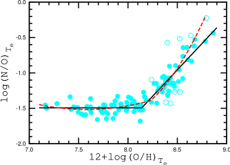
Figure 2: The O/H – N/O diagram for the calibration H ii regions. The solid (black) line shows a linear fit to the N/O – O/H relation (Eq. 7). The filled circles are data points used in deriving this relation, the open circles are rejected data points. The dashed (red) line shows an alternative quadratic fit to the N/O – O/H relation.

2.3 The O/H – N/O diagram

Fig. 2 shows a standard O/H – N/O diagram for the calibration H ii regions. Using these data, we have obtained the following linear relations between log N/O and log O/H

$$\begin{array}[]{lll}\log{\rm(N/O)}&=&-1.493\\ &&{\rm for}\quad 12+\log{\rm(O/H)}<8.14,\\ &&\\ &=&1.489\times(12+\log{\rm(O/H))}-13.613\\ &&{\rm for}\quad 12+\log{\rm(O/H)}>8.14.\\ \end{array}$$ (7)

Several H ii regions show large ($>$0.25 dex) abundance deviations. These have been excluded in deriving the final relation. In Fig. 2, the data points used in the derivation of the final relation (102 out of 112) are shown by filled circles, while the rejected data points are shown by open circles. The solid (black) line shows the derived relation. An alternate quadratic relation between log N/O and log O/H has also been derived:

$$\begin{array}[]{lll}\log{\rm(N/O)}&=&-1.39+0.39\,(Z-Z_{0})+0.30\,(Z-Z_{0})^{2}\\ &&{\rm for}\quad Z<8.23,\\ &&\\ &=&-1.39+1.24\,(Z-Z_{0})+1.63\,(Z-Z_{0})^{2}\\ &&{\rm for}\quad Z>8.23,\\ \end{array}$$ (13)

where $Z$ = 12 + log(O/H) and $Z_{0}$ = 8.23 (see the dashed (red) line in Fig. 2). The two relations are similar for metallicities 12 + log(O/H) $\la$ 8.5. We will here only consider objects in this metallicity range. Using the N/O – O/H relationship, one can estimate the N/O ratio which corresponds to a given oxygen abundance. The nitrogen-to-oxygen abundance ratio obtained in this way will be referred to as (N/O)_REL below. For definiteness, we will use the N/O – O/H relationship given by Eq. 7.

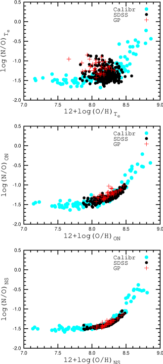
Figure 3: The O/H – N/O diagrams for SDSS objects (filled dark (black) circles), for the Green Pea galaxies (dark (red) plus signs), and for calibration H ii regions (filled grey (light-blue) circles) with abundances obtained with the $T_{e}$ method (upper panel), using the ON calibration (middle panel), and the NS calibration (lower panel). (A color version of this figure is available in the online version.)

We have derived (O/H)${}_{T_{e}}$, (O/H)_ON, (O/H)_NS oxygen abundances and (N/H)${}_{T_{e}}$, (N/H)_ON, and (N/H)_NS nitrogen abundances for all calibration H ii regions, SDSS and Green Pea galaxies. Fig. 3 shows the comparison between O/H – N/O diagrams for abundances computed in different ways.

The upper panel of Fig. 3 shows the O/H – N/O diagram for SDSS objects (filled dark (black) circles), Green Pea galaxies (dark (red) plus signs), and calibration H ii regions (filled grey (light-blue) circles) for abundances obtained with the $T_{e}$ method. The upper panel shows that some SDSS objects deviate significantly from the general trend defined by the calibration H ii regions: they are shifted towards higher N/O abundances ratio or/and towards lower O/H abundances. The same shift is observed for some Green Pea galaxies, in agreement with the findings of Amorín, Pérez-Montero & Vílchez (2010).

The middle panel of Fig. 3 shows the same O/H – N/O diagram, but for the case where abundances are obtained with the ON calibration, and shows that the SDSS and Green Pea galaxies follow the trend defined by the calibration H ii regions, without large deviations. The lower panel of Fig. 3 shows the NS calibration-based abundances. Again, the SDSS and Green Pea galaxies follow the trend defined by the calibration H ii regions and do not show large deviations.

Figure 4: The deviation of the N/O ratios in SDSS objects relative the N/O – O/H relation as a function of (1) the difference between $T_{e}$-based and ON-calibration-based oxygen abundances (upper panel), (2) of the flux in the auroral line [O iii]$\lambda$4363 normalised to the H$\beta$ line flux (middle panel), and (3) of the equivalent width EW([O iii]$\lambda$4363) of the auroral line (lower panel).

The upper panel of Fig. 4 shows the deviation of the (N/O)${}_{T_{e}}$ ratio in the SDSS objects from the N/O – O/H relation as a function of the difference between $T_{e}$-based and ON-calibration-based oxygen abundances. There is a clear anti-correlation between (log(N/O)${}_{T_{e}}$ – log(N/O)_REL) and (log(O/H)${}_{T_{e}}$ –log(O/H)_ON) values. This anti-correlation suggests the deviation of SDSS objects from the general N/O – O/H trend in the upper panel of Fig. 3 is mainly caused by shifts towards lower O/H abundances, i.e. the (O/H)${}_{T_{e}}$ abundances in these objects appear to be underestimated.

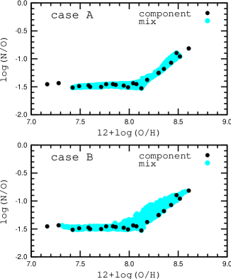
Figure 5: The O/H – N/O diagram for artificial composite nebulae and components. Upper panel. Filled dark (black) circles show the $T_{e}$-based abundances of components, while the grey (light-blue) filled circles are abundances of artificial composite nebulae, calculated as the mean luminosity-weighted abundance of all components, for case $A$. Lower panel. The same as in the upper panel, but for case $B$. (A color version of this figure is available in the online version.)

One may expect the high (N/O)${}_{T_{e}}$ ratios in SDSS objects to be caused by uncertainties in the flux of the weak auroral [O iii]$\lambda$4363 line in these objects. To check this hypothesis, we show in the middle panel of Fig. 4 the deviation of (N/O)${}_{T_{e}}$ ratios (log(N/O)${}_{T_{e}}$ – log(N/O)_REL) versus the flux of the [O iii]$\lambda$4363 auroral line, normalised to the H$\beta$ flux. The lower panel of Fig. 4 shows the deviation of the same (N/O)${}_{T_{e}}$ ratios as a function of the equivalent width EW([O iii]$\lambda$4363) of the [O iii]$\lambda$4363 auroral line. Examination of these two panels suggests that the uncertainties in the O iii]$\lambda$4363 line flux can indeed be responsible for a significant fraction of high (N/O)${}_{T_{e}}$ ratios in the SDSS galaxies. However, high (N/O)${}_{T_{e}}$ ratios are found not only in SDSS objects with a weak [O iii]$\lambda$4363 line, but also in some objects where that line is relatively strong, with EW([O iii]$\lambda$4363) $>$ 5 and/or [O iii]$\lambda$4363/H$\beta$ $>$ 0.05. This implies that the auroral line flux uncertainties cannot be the only reason for the high (N/O)${}_{T_{e}}$ ratios found in some SDSS objects.

We propose here another explanation for the derived high (N/O)${}_{T_{e}}$ ratios. SDSS galaxies are composite nebulae which contain a number of H ii regions with different physical properties, all contributing to the global spectrum. In that case, the meaning of a single measured electron temperature for the whole galaxy is not well defined and consequently, $T_{e}$-based abundances are ambiguous. We expect the electron temperature estimated from the auroral-to-nebular lines ratio to be overestimated and the derived oxygen abundance to be underestimated. In other words, such nebulae will exhibit an effect similar to the temperature fluctuations discussed by Peimbert (1967). However, these temperature variations will not occur within a single H ii region, but on the large scale, in ongoing from one H ii region to other. These temperature variations in an object will cause it to deviate from the general N/O – O/H trend. To explore this scenario quantitatively, we use a Monte Carlo simulation to construct spectra of composite nebulae (described in the next section), and examine how derived abundances in composite nebulae change, depending on the abundance determination method.

3 Global abundances in artificial composite nebulae

3.1 Monte Carlo simulation of global spectra

To clarify the reason for the discrepancy between the $T_{e}$-based and calibration-based abundances in our sample of distant SDSS galaxies, we have simulated their spectra. We have remarked above that several different H ii regions can contribute to the global spectra of distant SDSS galaxies. We have modelled their global spectra by using the approach of Pilyugin, Contini, & Vílchez (2004a); Pilyugin et al. (2010a). The artificial spectra of SDSS galaxies have been computed as a mix of spectra of individual components, which we take to be spectra of real H ii regions in nearby galaxies with measured electron temperatures, taken from the calibration H ii region sample.

The auroral line [O iii]$\lambda$4363 is usually detected in spectra of low-metallicity calibration H ii regions and $t_{3}$ can then be determined, while the auroral line [N ii]$\lambda$5755 is detected in spectra of high-metallicity calibration H ii regions, resulting in the determination of $t_{2}$. When [N ii]$\lambda$5755 is detected in the spectrum of an H ii region, then the intensity of [O iii]$\lambda$4363 is estimated in the following manner. We calculate $t_{3}$ from the measured $t_{2}$ using the $t_{2}$ – $t_{3}$ relation. We then estimate the line flux of [O iii]$\lambda$4363 corresponding to the obtained value of t₃.

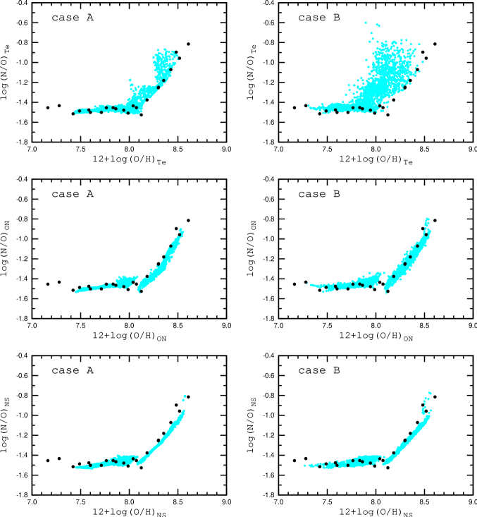
Figure 6: The O/H – N/O diagrams for the artificial composite nebulae for case $A$ (left panels) and for case $B$ (right panels). The grey (light-blue) filled circles show the abundances derived in different ways from artificial global spectra. The dark (black) filled circles are $T_{e}$-based abundances in the components. (A color version of this figure is available in the online version.)

Using the calibration H ii regions as components, we have performed a variety of Monte Carlo simulations, producing in each run an artificial spectrum of a composite nebula. The calibration H ii regions are not distributed uniformly within the considered metallicity range. We have thus divided the metallicity range in bins of $\Delta$(log(O/H)) = 0.05 and selected one calibration H ii region within each bin according to the following two criteria:

1. The average value of the difference between the calibration-based and $T_{e}$ - based abundances is minimum. Both oxygen and nitrogen abundances and both ON and NS calibrations were taken into account in determining the average value of the difference.
   

2. The deviation of N/O abundances ratio from the N/O – O/H relation is not in excess of 0.15 dex.

Fig. 5 shows the positions of the selected calibration H ii regions in the O/H – N/O diagram by dark (black) filled circles.

At a fixed 12+log(O/H)₀, we have simulated 100 global spectra, using the spectra of selected calibration H ii regions with oxygen abundances within 12+log(O/H)₀ $\pm$ $\Delta$(log(O/H)). The contribution from each component to a given global spectrum of artificial composite H ii regions is defined by the value $w_{\rm j}$, where $w_{\rm j}$ are random numbers between -1 and 1. To take into account that some components may not contribute to a given spectrum we choose the interval of random numbers between -1 and 1 instead of the standard interval between 0 and 1 and when $w_{\rm j}<0$ we set it to 0, i.e. the component does not make contribution to the global spectrum. The component (calibration H ii region) line fluxes are given on a scale where $F($H${\beta})=1$, therefore we can consider that the value $w_{\rm j}$ defines H${\beta}$ flux (or luminosity) of $j$ component in the given variant of the global spectra. Then the total $F($H${\beta})$ flux of the composite nebula is given by the expression:

$$F({\rm H}{\beta})=\sum\limits_{{\rm j}=1}^{{\rm j}={\rm n}}w_{\rm j},$$ (14)

where $n$ is the number of components in the composite nebula.

The flux $F($X${}_{\lambda_{\rm k}})$ of the composite nebula in the line X${}_{\lambda_{\rm k}}$ is given by:

$$F({\rm X}_{\lambda_{\rm k}})=\frac{\sum\limits_{{\rm j}=1}^{{\rm j}={\rm n}}w_{\rm j}F_{\rm j}({\rm X}_{\lambda_{\rm k}})}{\sum\limits_{{\rm j}=1}^{{\rm j}={\rm n}}w_{\rm j}}.$$ (15)

We have computed the intensity of the H${\beta}$, [O ii]$\lambda$3727, [O iii]$\lambda$4363, [O iii]$\lambda$4959, [O iii]$\lambda$5007, [N ii]$\lambda$6548, [N ii]$\lambda$6584, [S ii]$\lambda$6717, and [S ii]$\lambda$6731 lines for the each artificial spectrum of composite nebulae.

The mean oxygen abundance of a composite H ii region, weighted by the H$\beta$ line luminosity, can be determined as

$${\rm(O/H)}_{mean}=\frac{\sum\limits_{{\rm j}=1}^{{\rm j}={\rm n}}w_{\rm j}{\rm(O/H)_{j}}}{\sum\limits_{{\rm j}=1}^{{\rm j}={\rm n}}w_{\rm j}}.$$ (16)

Similarly, the mean nitrogen abundance in a composite H ii region is given by

$${\rm(N/H)}_{mean}=\frac{\sum\limits_{{\rm j}=1}^{{\rm j}={\rm n}}w_{\rm j}{\rm(N/H)_{j}}}{\sum\limits_{{\rm j}=1}^{{\rm j}={\rm n}}w_{\rm j}}.$$ (17)

For each computed spectrum, we have estimated $t_{3}$, (O/H)_mean, (N/H)_mean, (O/H)${}_{T_{e}}$, (N/H)${}_{T_{e}}$, (O/H)_NS, (N/H)_NS, (O/H)_ON and (N/H)_ON abundances. This procedure was repeated for a variety of 12+log(O/H)₀ values .

3.2 Global abundances in artificial composite nebulae

Here, we discuss two cases, represented by two sets of Monte Carlo simulations:

• We simulated 100 global spectra for each 12+log(O/H)₀, using components with oxygen abundances within 12+log(O/H)₀ $\pm$ 0.15, and varying 12+log(O/H)₀ from 7.5 to 8.5 in steps of 0.05 dex. The grey (light-blue) filled circles in the upper panel of Fig. 5 show the mean abundances of the artificial composite nebulae for case $A$. The abundances of each component has been weighted by the corresponding H$\beta$-luminosities.
  

• We simulated 100 global spectra for each 12+log(O/H)₀, using components with oxygen abundances within 12+log(O/H)₀ $\pm$ 0.35. The grey (light-blue) filled circles in the lower panel of Fig. 5 show the mean abundances in artificial composite nebulae for case $B$.

The N/O – O/H diagrams for case $A$ with abundances obtained in different ways from the global spectra are shown in the left panels of Fig. 6 by grey (light-blue) filled circles. The upper panel shows the $T_{e}$-based abundances, the middle panel the ON-calibration-based abundances, and the lower panel the NS-calibration-based abundances in the artificial composite nebulae. The dark (black) filled circles in each panel are the $T_{e}$-based abundances of each component. The upper left panel shows that a significant fraction of the artificial composite nebulae with $T_{e}$ - based abundances are shifted from the O/H – N/O relation towards higher N/O ratios or/and towards lower oxygen abundances.

The left upper panel of Fig. 7 shows the difference between nitrogen-to-oxygen ratios (N/O)${}_{T_{e}}$ and (N/O)_mean in the artificial composite nebulae as a function of the difference between oxygen abundances (O/H)${}_{T_{e}}$ and (O/H)_mean for case $A$ by the grey (light-blue) filled circles. The dark (black) filled circles show the components. The right upper panel of Fig. 7 shows the deviation of (N/O)${}_{T_{e}}$ ratios in the artificial composite nebulae from the N/O – O/H relation (the linear fit discussed previously) as a function of the difference between the oxygen abundance derived by the $T_{e}$ method from global spectra and that obtained as the H$\beta$-luminosity-weighted mean abundances of components for case $A$.

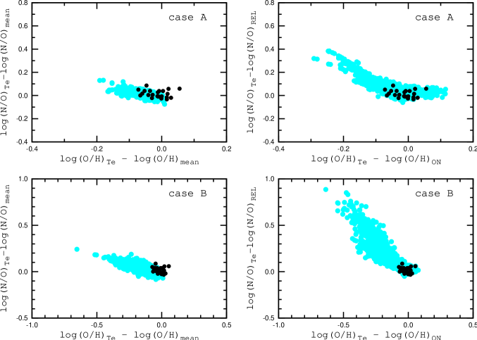
Figure 7: Left upper panel. The grey (light-blue) filled circles show the difference between nitrogen-to-oxygen ratios (N/O)${}_{T_{e}}$ and (N/O)_mean in artificial composite nebulae as a function of the difference between oxygen abundances (O/H)${}_{T_{e}}$ – (O/H)_mean foe case $A$. The dark (black) filled circles show the components. Right upper panel. The grey (light-blue) filled circles show the deviation of (N/O)${}_{T_{e}}$ ratios in artificial composite nebulae from the expected N/O – O/H relation as a function of the difference between oxygen abundances derived with the $T_{e}$ method from global spectra and those obtained through ON calibration. Lower panels show the same but for case $B$. (A color version of this figure is available in the online version.)

The N/O – O/H diagram of $T_{e}$-based abundances for artificial composite nebulae for case $B$ is shown in the upper right panel of Fig. 6 by the dark (black) filled circles. The grey (light-blue) filled circles are $T_{e}$-based abundances of the components. Again, a fraction of artificial composite nebulae with $T_{e}$-based abundances are shifted from the O/H – N/O relation towards higher N/O ratios or/and towards lower oxygen abundances. The grey (light-blue) filled circles in the lower left panel of Fig. 7 shows the difference between nitrogen-to-oxygen ratios (N/O)${}_{T_{e}}$ and (N/O)_mean in artificial composite nebulae as a function of the difference between oxygen abundances (O/H)${}_{T_{e}}$ and (O/H)_mean for case $B$. The dark (black) filled circles show the individual components. The lower right panel of Fig. 7 shows the deviations of (N/O)${}_{T_{e}}$ ratios in the artificial composite nebulae from the N/O – O/H relation (the linear fit discussed previously) as a function of the difference between the oxygen abundance derived by the $T_{e}$ method from global spectra and that obtained as the H$\beta$-luminosity-weighted mean abundances of components for case $B$.

By comparison of Fig. 4 and Fig. 7 it is evident that artificial composite nebulae reproduce the anti-correlation between (log(N/O)${}_{T_{e}}$ – log(N/O)_REL) and (log(O/H)${}_{T_{e}}$ – log(O/H)_ON) observed in our sample of SDSS galaxies. This can be considered in favour of our hypothesis that the enhanced (N/O)${}_{T_{e}}$ ratio derived for some SDSS objects can be due to the fact that these objects are composite nebulae, with a number of H ii regions with different physical properties contributing to the global spectrum. Hence, the electron temperature determined from the auroral-to-nebular lines ratio is overestimated, and the oxygen abundance is underestimated in such a nebula, i.e., it appears to be a Peimbert temperature fluctuation effect (see the introduction).

The middle and lower panels of Fig. 6 show that both the ON and NS calibration-based abundances in the artificial composite nebulae follow, in general, the abundances of the components. However, both case A and B show a gap near 12+log(O/H) $\sim$ 8.1. This gap is due to a transition between two regimes in the calibrations, i.e., by the fact that both “warm” and “hot” H ii regions (according to the classification in Pilyugin et al., 2010b)) make contributions to the global spectrum of composite nebulae. Therefore, such composite H ii regions are neither purely warm nor purely hot. But distinct calibration relations for warm and hot H ii regions were in fact used (Pilyugin et al., 2010b; Pilyugin & Mattsson, 2011). Hence, there appears to be a problem regarding how these calibration relations should be applied to such nebulae. It should also be noted that the criterion for distinguishing between warm and hot H ii regions is somewhat arbitrary.

We have performed a variety of Monte Carlo simulations, using different sets of components and different $\Delta$(log(O/H)) intervals, to produce artificial global spectra. We have found that the underestimation of the oxygen abundance with the $T_{e}$ method – and, consequently, the shift of the position in the N/O – O/H diagram of the artificial composite nebula with $T_{e}$-based abundances relative to its position with mean oxygen and nitrogen abundances – is larger for nebulae where the components have large differences in physical properties. In particular, the value of the shift increases with increasing $\Delta$(log(O/H). Thus, we have reached the following conclusions:

• If the composite nebula consists of H ii regions with similar physical properties or a single H ii region which makes a dominant contribution to the global spectrum, then the oxygen and nitrogen abundances derived with the $T_{e}$ method and the ON and NS calibrations are in satisfactory agreement with each other, and near the mean H$\beta$ luminosity weighted oxygen and nitrogen abundances of the components in the composite nebula.
  

• If H ii regions with different physical properties make comparable contributions to the global spectrum of the composite nebula, then the $T_{e}$ - based oxygen abundance can be underestimated. Hence, the position of such a nebula in the N/O – O/H diagram will be shifted towards lower oxygen abundances, mimicking an enhancement of the N/O ratio.
  

• The ON and NS calibrations give oxygen and nitrogen abundances in the composite nebulae which agree with the mean luminosity-weighted abundances of their components to within $\sim$0.2 dex.

It should be noted that the high-metallicity (12+log(O/H) $\ga$ 8.5) calibration H ii regions with measured electron temperatures are very few. Thus, they cannot be simulated and we cannot investigate how similar (or dissimilar) their abundances estimated using the $T_{e}$ method and the strong-line calibrations are. Furthermore, our approach does not allow to take into account the contribution of a diffuse emission.

4 DISCUSSION

Our conclusion that the global abundances derived for composite nebulae with the classic $T_{e}$ method may be subject to systematic errors is not surprising. First, an effect of this kind has been predicted by Peimbert (1967) for H ii regions with a non-uniform electron temperature. Second, Kobulnicky et al. (1999) have compared physical conditions derived from spectroscopy of individual H ii regions with those obtained from global spectroscopy for several galaxies with 12 + log(O/H)$\sim 8.2$, and where the auroral line [O iii]$\lambda$4363 is detected in both individual and global spectra. They found that the standard $T_{e}$ method using global spectra give systematic errors in that the oxygen abundances derived from global spectra are systematically 0.05 – 0.2 dex below the median values computed from spectra obtained in smaller apertures.

The global oxygen abundances estimated with the one-dimensional $R_{23}$ calibration have been discussed by Kobulnicky et al. (1999); Moustakas & Kennicutt (2006), while those obtained with the two dimensional $R_{23}$ calibration ($P$ method) have been discussed by Pilyugin, Contini, & Vílchez (2004a). It has been found that the abundance inferred from the integrated emission-line spectrum of a galaxy using one- or two-dimensional $R_{23}$ calibrations is representative of the gas-phase oxygen abundance at a fixed galactocentric radius (equal to 0.4 times the isophotal radius), as determined by the abundance gradient derived from H ii regions. Here, we have found that the global abundances derived using the ON and NS calibrations are close to the mean abundances. Thus, the calibrations produce robust global abundances although both the absolute values of abundances in individual H ii regions and of global abundances depend on the adopted calibration.

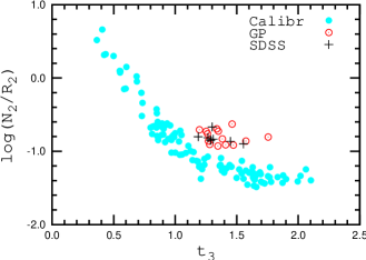
Figure 8: The flux ratio $N_{2}/R_{2}$ as a function of electron temperature $t_{3}$. The grey (ligh-blue) filled circles show the calibration H ii regions. The SDSS objects with large ($>$ 0.3 dex) deviations from the expected N/O – O/H relation are shown by dark (black) plus signs. The Green Pea galaxies with large deviations from the expected N/O – O/H relation are shown by open (red) circles. (A color version of this figure is available in the online version.)

Figure 9: Electron temperature $t_{3}$ as a function of oxygen abundance for the calibration H ii regions.

Our results suggest the $T_{e}$-based abundances in some composite nebulae can be incorrect and shift the positions of these nebulae in the O/H – N/O diagram towards higher N/O abundances ratio or/and towards lower O/H abundances relatively to the positions of H ii regions in nearby galaxies. Thus the high (N/O)${}_{T_{e}}$ abundances ratios obtained in some SDSS and Green Pea galaxies may be incorrect because they are composite nebulae.

Fig. 8 shows the $N_{2}/R_{2}$ flux ratios as a function of the electron temperature $t_{3}$ for the calibration H ii regions and for the SDSS and Green Pea galaxies with large ($>$ 0.3 dex) deviations from the expected N/O – O/H relation. In the ON calibration, the $N_{2}/R_{2}$ flux ratios are used as temperature indicators. Fig. 8 shows that the measured $N_{2}/R_{2}$ in SDSS and Green Pea galaxies with $t_{3}$ $\sim$1.4 have values that are more typical for nebulae with $t_{3}$ $\sim$1. This means the two electron temperature indicators ([O iii]$\lambda$4959,$\lambda$5007/[O iii]$\lambda$4363 and $N_{2}/R_{2}$) are in conflict. Thus, to reproduce both the measured electron temperature $t_{3}$ and the $N_{2}/R_{2}$ flux ratios, the composite nebula should contain a component with a temperature $t_{3}$ $\sim$1 as well as one with $t_{3}$ $\ga$ 1.4. The temperature difference between components can be larger than 5000 K, in some cases. For example, the hottest Green Pea galaxy in our sample (with a large N/O deviation), J012910.15 + 145934.6, has $t_{3}$ = 1.75 while its measured $N_{2}/R_{2}$ flux ratio is typical for a nebula with $t_{3}$ $\sim$1.

Fig. 9 shows $t_{3}$ as a function of the oxygen abundance 12+log(O/H) for the calibration H ii regions. We see that a H ii region with $t_{3}$ $\sim$1 has 12+log(O/H) $\sim$8.3. Can a hot component of metallicity 12+log(O/H) $\sim$ 8.3 be responsible for the high $t_{3}$ value ($\sim$ 1.4) in the composite nebula?

We can expect the points in the $t_{3}$ – O/H diagram (Fig. 9) to be close to the highest attainable electron temperatures $t_{3}$ for a given 12+log(O/H) because of a selection effect: electron temperatures are easiest to measure in the hottest H ii regions. In such case, an H ii region of metallicity log(O/H) = 8.3 cannot have an electron temperature as high as $t_{3}$ $\sim$ 1.4. Thus, a hot component with 12+log(O/H) $\sim$8.3 cannot be responsible for the high electron temperature measured.

According to Fig. 9, a H ii region with $t_{3}$ $\sim$1.4 has 12+log(O/H) $\sim$8.0. Furthermore, the $N_{2}/R_{2}$ flux ratio increases with decreasing electron temperature. Can a cold component with 12+log(O/H) $\sim$8.0 be responsible for the high $N_{2}/R_{2}$?

The typical N/O ratio in H ii regions with log(O/H) $\sim$ 8.0 is log(N/O) $\sim-1.5$. A H ii region with log(O/H) $\sim$ 8.0 and log(N/O) = –1.5 would have log$N_{2}/R_{2}=-0.9$ at $t_{3}$ $\sim$0.5. However, the line fluxes $N_{2}$ and $R_{2}$ (normalised to the H$\beta$ flux) are one order of magnitude lower than the measured fluxes. Thus, a cold component of metallicity 12+log(O/H) $\sim$8.0 cannot be responsible for the high $N_{2}/R_{2}$ flux ratio measured.

The measured high N/O ratios and high electron temperatures in some SDSS and Green Pea galaxies can be reproduced by composite nebulae involving components of different metallicities. However, the metallicity difference can be as large as a factor 2-3, or even larger in extreme cases. It is believed that Green Peas are low-mass galaxies (Cardamone et al., 2009; Amorín, Pérez-Montero & Vílchez, 2010; Izotov et al., 2011). The metallicity scatter of H ii regions in typical dwarf galaxies is known to be small (e.g. Croxall et al., 2009). This suggests that the measured high N/O ratios not in all the Green Pea galaxies can be reproduced by composite nebulae and some Green Pea galaxies may not be typical dwarfs galaxies. A large metallicity scatter of the H ii regions in a dwarf galaxy can arise if this galaxy has undergone an atypical evolution. For example, it can be the result of the merging of two dwarfs of different metallicities, triggering a starburst in both components simultaneously. Infall of non-enriched gas onto a well-evolved galaxy with a high N/O gas-phase ratio would decrease the oxygen and nitrogen abundances, and would result in a galaxy with an enhanced N/O ratio. The evolution of a galaxy with selective heavy elements loss through enriched galactic winds can also result in enhanced N/O ratios (e.g. Pilyugin, 1993; Yin, Matteucci, & Vladilo, 2011).

5 CONCLUSIONS

We have examined the oxygen and nitrogen abundances derived from global emission-line spectra of galaxies with 12 + log(O/H) ranging from $\sim$7.5 to $\sim$8.5, based on a sample of 281 SDSS galaxies with measured electron temperatures. The oxygen and nitrogen abundances in these galaxies were derived with the $T_{e}$ method as well as with two recent strong-line calibrations: the ON and NS calibrations.

For $T_{e}$-based abundances, the positions of some SDSS galaxies in the O/H – N/O diagram are shifted towards higher N/O ratios or/and towards lower O/H abundances relative to the positions of H ii regions in nearby galaxies. In case of strong-line calibration-based abundances, the SDSS galaxies occupy the same area in the O/H – N/O diagram as the H ii regions in nearby galaxies.

The global spectra of galaxies have been Monte Carlo simulated as a mix of spectra of individual components, based on well-observed H ii regions in nearby galaxies. Abundance analysis of the artificial composite nebulae yields the following conclusions:

1. If the composite nebula consists of H ii regions with similar physical properties or a single H ii region makes a dominant contribution to the global spectrum, then the oxygen and nitrogen abundances derived with the $T_{e}$ method and the ON and NS calibrations are in satisfactory agreement with each other and near the mean H$\beta$ luminosity weighted value of oxygen and nitrogen abundances of the individual components of the composite nebula.

2. If H ii regions with different physical properties make comparable contributions to the global spectrum, then the $T_{e}$ - based oxygen abundances may be underestimated and the position of such a nebula in the N/O – O/H diagram will be shifted towards lower oxygen abundances, mimicking an enhancement of the N/O ratio in the nebula. This effect is similar to the one discussed by Peimbert for H ii regions with small scale temperature fluctuations. For composite nebulae however, this effect appears to be due to temperature variations on large spatial scales, caused by varying temperatures in different components of the composite nebula.

3. The ON and NS calibrations give oxygen and nitrogen abundances in composite nebulae which agree with the mean luminosity-weighted abundances of their components to within $\sim$0.2 dex. ON- and NS-calibration-based abundances for these nebulae also show a gap in abundance near 12+log(O/H) $\sim$ 8.1.

4. The high (N/O)${}_{T_{e}}$ ratios derived in some Green Pea galaxies may be caused by the fact that their SDSS spectra are spectra of composite nebulae made up of several components with different physical properties (such as metallicity). However, for the hottest Green Pea galaxies, which appear to be dwarf galaxies, this explanation does not seem to be plausible. It would work only if the HII regions in these galaxies have a dispersion of abundances much larger than that typically found in dwarf galaxies.

References

- Alloin et al. (1979) Alloin D., Collin-Souffrin S., Joly M., Vigroux L., 1979, A&A, 78, 200
- Amorín, Pérez-Montero & Vílchez (2010) Amorín R.O., Pérez-Montero E., Vílchez J.M., 2010, ApJ, 715, L128
- Asari et al. (2007) Asari N.V., Cid Fernandes R., Stasińska G., Torres-Papaqui J.P., Mateus A., Sodré L., Schoenell W., 2007, MNRAS, 381, 263
- Bresolin, Kennicutt, & Garnett (1999) Bresolin F., Kennicutt R.C., Jr., Garnett D.R., 1999, ApJ, 510, 104
- Bresolin et al. (2005) Bresolin F., Shaerer D., González Delgado R.M., Stasińska G., 2005, A&A, 441, 981
- Bresolin (2007) Bresolin F., 2007, ApJ, 656, 186
- Bresolin et al. (2009) Bresolin F., Gieren W., Kudritzki R.-P., Pietrzyński G., Urbaneja M.A., Carraro G., 2009, ApJ, 700, 309
- Campbell, Terlevich & Melnick (1986) Campbell A., Terlevich R., Melnick J., 1986, MNRAS, 223, 811
- Cardamone et al. (2009) Cardamone C., Schawinski K., Sarzi M., et al., 2009, MNRAS, 399, 1191
- Croxall et al. (2009) Croxall K.V., van Zee L., Lee H., Skillman E.D., Lee J.C., Côté S., Kennicutt R.C., Jr. Miller B.W., 2009, ApJ, 705, 723
- Denicolo, Terlevich & Terlevich (2002) Denicolo G., Terlevich R., Terlevich E., 2002, MNRAS, 330, 69
- Dopita & Evans (1986) Dopita M.A., Evans I.N., 1986, ApJ, 307, 431
- Erb et al. (2006) Erb D.K., Shapley A.E., Pettini M., Steidel C.C., Reddy N.A., Adelberger K.L., 2006, ApJ, 644, 813
- Ercolano et al. (2007) Ercolano B., Bastian N., Stasińska G., 2007, MNRAS, 379, 945
- Ercolano et al. (2010) Ercolano B., Wesson R., & Bastian N. 2010, MNRAS, 401, 1375
- Garnett (1992) Garnett D.R. 1992, AJ, 103, 1330
- Izotov et al. (2006) Izotov Y.I., Stasińska G., Meynet G., Guseva N.G., Thuan T.X., 2006, A&A, 448, 955
- Izotov et al. (2011) Izotov Y.I., Guseva N.G., Thuan T.X., 2011, ApJ, 728, 161
- Kennicutt (1992) Kennicutt R.C., (Jr.), 1992, ApJ, 338, 310
- Kniazev et al. (2004) Kniazev A.Y., Pustilnik S.A., Grebel E.K., Lee H., Pramskij A.G., 2004, ApJS, 153, 429
- Kobulnicky et al. (1999) Kobulnicky H.A., Kennicutt R.C., (Jr.), Pizagno J.L., 1999, ApJ, 514, 544
- Liang et al. (2006) Liang Y.C., Yin S.Y., Hammer F., Deng L.C., Flores H., Zhang B., 2006, ApJ, 652, 257
- McCall, Rybski & Shields (1985) McCall M.L., Rybski P.M., Shields G.A., 1985, ApJS, 57, 1
- Moustakas & Kennicutt (2006) Moustakas J., Kennicutt R.C., (Jr), 2006, ApJ, 651, 155
- Pagel et al. (1979) Pagel B.E.J., Edmunds M.G., Blackwell D.E., Chun M.S., Smith G., 1979, MNRAS, 189, 95
- Peimbert (1967) Peimbert M., 1967, ApJ, 150, 825
- Pettini & Pagel (2004) Pettini M., Pagel B.E.J., 2004, MNRAS, 348, 59L
- Pérez-Montero & Contini (2009) Pérez-Montero E., Contini T., 2009, MNRAS, 398, 949
- Pilyugin (1993) Pilyugin L.S., 1993, A&A, 277, 42
- Pilyugin (2000) Pilyugin L.S., 2000, A&A, 362, 325
- Pilyugin (2001) Pilyugin L.S., 2001, A&A, 369, 594
- Pilyugin, Contini, & Vílchez (2004a) Pilyugin L.S., Contini T., Vílchez J.M., 2004a, A&A, 423, 427