A uniform inf–sup condition with applications to preconditioning

Abstract.

A uniform inf–sup condition related to a parameter dependent Stokes problem is established. Such conditions are intimately connected to the construction of uniform preconditioners for the problem, i.e., preconditioners which behave uniformly well with respect to variations in the model parameter as well as the discretization parameter. For the present model, similar results have been derived before, but only by utilizing extra regularity ensured by convexity of the domain. The purpose of this paper is to remove this artificial assumption. As a byproduct of our analysis, in the two dimensional case we also construct a new projection operator for the Taylor–Hood element which is uniformly bounded in $L^{2}$ and commutes with the divergence operator. This construction is based on a tight connection between a subspace of the Taylor–Hood velocity space and the lowest order Nedelec edge element.

1. Introduction

The purpose of this paper is to discuss preconditioners for finite element discretizations of a singular perturbation problem related to the linear Stokes problem. More precisely, let $\Omega\subset\mathbb{R}^{n}$ be a bounded Lipschitz domain and $\operatorname{\epsilon}\in(0,1]$ a real parameter. We will consider singular perturbation problems of the form

(1.1) $$\begin{array}[]{rl}(I-\operatorname{\epsilon}^{2}\Delta)u-\operatorname{grad}p&=f\quad\text{in }\Omega,\\ \operatorname{div}u&=g\quad\text{in }\Omega,\\ u&=0\quad\text{on }\partial\Omega,\end{array}$$

where the unknowns $u$ and $p$ are a vector field and a scalar field, respectively. For each fixed positive value of the perturbation parameter $\operatorname{\epsilon}$ the problem behaves like the Stokes system, but formally the system approaches a so–called mixed formulation of a scalar Laplace equation as this parameter tends to zero. In physical terms this means that we are studying fluid flow in regimes ranging from linear Stokes flow to porous medium flow. Another motivation for studying preconditioners of these systems is that they frequently arises as subsystems in time stepping schemes for time dependent Stokes and Navier–Stokes systems, cf. for example [3, 6, 16, 18, 19].

The phrase uniform preconditioners for parameter dependent problems like the ones we discuss here, refers to the ambition to construct preconditioners such that the preconditioned systems have condition numbers which are bounded uniformly with respect to the perturbation parameter $\operatorname{\epsilon}$ and the discretization. Such results have been obtained for the system(1.1) in several of the studies mentioned above, but a necessary assumption in all the studies so far has been a convexity assumption on the domain, cf. [17]. However, below in Section 3 we will present a numerical example which clearly indicates that this assumption should not be necessary. Thereafter, we will give a theoretical justification for this claim. The basic tool for achieving this is to introduce the Bogovskiĭ operator, cf. [8], as the proper right inverse of the divergence operator in the continuous case.

The construction of uniform preconditioners for discretizations of systems of the form (1.1), is intimately connection to the well–posedness properties of the continuous system, and the stability of the discretization. In fact, if we obtain appropriate $\operatorname{\epsilon}$–independent bounds on the solution operator, then the basic structure of a uniform preconditioner for the continuous system is an immediate consequence. Furthermore, under the assumption of proper stability properties of the discretizations, the basic structure of uniform preconditioners for the discrete system also follows. We refer to [15] and references given there for a discussion of these issues. The main tool for analyzing the well–posedness properties of saddle–point problems of the form (1.1) is the Brezzi conditions, cf. [4, 5]. In particular, the desired uniform bounds on the solution operator is closely tied to a uniform inf–sup condition of the form (2.4) stated below. Furthermore, the verification of such uniform conditions are closely tied to the construction of uniformly bounded projection operators which properly commute with the divergence operator. In the present case, these projection operators have to be bounded both in $L^{2}$ and in $H^{1}$. In Section 4 we will construct such operators in the case of the Mini element and the Taylor–Hood element, where the latter construction is restricted to quasi–uniform meshes in two space dimensions.

2. Preliminaries

To state the proper uniform inf–sup condition for the system (1.1) we will need some notation. If $X$ is a Hilbert space, then $\|\cdot\|_{X}$ denotes its norm. We will use $H^{m}=H^{m}(\Omega)$ to denote the Sobolev space of functions on $\Omega$ with $m$ derivatives in $L^{2}=L^{2}(\Omega)$. The corresponding spaces for vector fields are denoted $H^{m}(\Omega;\mathbb{R}^{n})$ and $L^{2}(\Omega;\mathbb{R}^{n})$. Furthermore, $\langle\cdot,\cdot\rangle$ is used to denote the inner–products in both $L^{2}(\Omega)$ and $L^{2}(\Omega;\mathbb{R}^{n})$, and it will also denote various duality pairings obtained by extending these inner–products. In general, we will use $H^{m}_{0}$ to denote the closure in $H^{m}$ of the space of smooth functions with compact support in $\Omega$, and the dual space of $H^{m}_{0}$ with respect to the $L^{2}$ inner product by $H^{-m}$. Furthermore, $L^{2}_{0}$ will denote the space of $L^{2}$ functions with mean value zero. We will use ${\mathcal{L}}(X,Y)$ to denote the space of bounded linear operators mapping elements of $X$ to $Y$, and if $Y=X$ we simply write ${\mathcal{L}}(X)$ instead of ${\mathcal{L}}(X,X)$.

If $X$ and $Y$ are Hilbert spaces, both continuously contained in some larger Hilbert space, then the intersection $X\cap Y$ and the sum $X+Y$ are both Hilbert spaces with norms given by

$$\|x\|_{X\cap Y}^{2}=\|x\|_{X}^{2}+\|x\|_{Y}^{2}\quad\text{and }\|z\|_{X+Y}^{2}=\inf_{\begin{subarray}{c}x\in X,y\in Y\\ z=x+y\end{subarray}}(\|x\|_{X}^{2}+\|y\|_{Y}^{2}).$$

Furthermore, if $X\cap Y$ are dense in both the Hilbert spaces $X$ and $Y$ then $(X\cap Y)^{*}=X^{*}+Y^{*}$ and $(X+Y)^{*}=X^{*}\cap Y^{*}$, cf. [2].

The system (1.1) admits the following weak formulation:

Find $(u,p)\in H_{0}^{1}(\Omega;\mathbb{R}^{n})\times L^{2}_{0}(\Omega)$ such that

(2.1) $$\begin{array}[]{rll}\langle u,v\rangle+\operatorname{\epsilon}^{2}\langle Du,Dv\rangle&+\,\langle p,\operatorname{div}v\rangle&=\langle f,v\rangle,\quad v\in H_{0}^{1}(\Omega;\mathbb{R}^{n}),\\ \langle\operatorname{div}u,q\rangle&&=\langle g,q\rangle,\quad q\in L^{2}_{0}(\Omega)\end{array}$$

for given data $f$ and $g$. Here $Dv$ denotes the gradient of the vector field $v$. More compactly, we can write this system in the form

(2.2) $${\mathcal{A}}_{\operatorname{\epsilon}}\begin{pmatrix}u\\ p\end{pmatrix}=\begin{pmatrix}f\\ g\end{pmatrix},\quad\text{where }{\mathcal{A}}_{\operatorname{\epsilon}}=\begin{pmatrix}I-\operatorname{\epsilon}^{2}\Delta&-\operatorname{grad}\\ \operatorname{div}&0\end{pmatrix}.$$

For each fixed positive $\operatorname{\epsilon}$ the coefficient operator ${\mathcal{A}}_{\operatorname{\epsilon}}$ is an isomorphism mapping $X=H_{0}^{1}(\Omega;\mathbb{R}^{n})\times L^{2}_{0}(\Omega)$ onto $X^{*}=H^{-1}(\Omega;\mathbb{R}^{n})\times L^{2}_{0}(\Omega)$. However, the operator norm $\|{\mathcal{A}}_{\operatorname{\epsilon}}^{-1}\|_{{\mathcal{L}}(X^{*},X)}$ will blow up as $\operatorname{\epsilon}$ tends to zero.

To obtain a proper uniform bound on the operator norm for the solution operator ${\mathcal{A}}_{\operatorname{\epsilon}}^{-1}$ we are forced to introduce $\operatorname{\epsilon}$ dependent spaces and norms. We define the spaces $X_{\operatorname{\epsilon}}$ and $X_{\operatorname{\epsilon}}^{*}$ by

$$X_{\operatorname{\epsilon}}=(L^{2}\cap\operatorname{\epsilon}H^{1}_{0})(\Omega;\mathbb{R}^{n})\times((H^{1}\cap L^{2}_{0})+\operatorname{\epsilon}^{-1}L_{0}^{2})(\Omega)$$

and

$$X_{\operatorname{\epsilon}}^{*}=(L^{2}+\operatorname{\epsilon}^{-1}H^{-1})(\Omega;\mathbb{R}^{n})\times(H^{-1}_{0}\cap\operatorname{\epsilon}L^{2}_{0})(\Omega).$$

Here $H^{-1}_{0}\supset L^{2}_{0}$ corresponds to the dual space of $H^{1}\cap L^{2}_{0}$. Note that the space $X_{\operatorname{\epsilon}}$ is equal to $X$ as a set, but the norm approaches the $L^{2}$–norm as $\operatorname{\epsilon}$ tends to zero.

Our strategy is to use the Brezzi conditions [4, 5] to claim that the operator norms

(2.3) $$\|{\mathcal{A}}_{\operatorname{\epsilon}}\|_{{\mathcal{L}}(X_{\operatorname{\epsilon}},X_{\operatorname{\epsilon}}^{*})}\quad\text{and }\|{\mathcal{A}}_{\operatorname{\epsilon}}^{-1}\|_{{\mathcal{L}}(X_{\operatorname{\epsilon}}^{*},X_{\operatorname{\epsilon}})}\quad\text{are bounded independently of }\operatorname{\epsilon}.$$

In fact, the only nontrivial condition for obtaining this is that we need to verify the uniform inf–sup condition

(2.4) $$\sup_{v\in H_{0}^{1}(\Omega;\mathbb{R}^{n})}\frac{\langle\operatorname{div}v,q\rangle}{\|v\|_{L^{2}\cap\operatorname{\epsilon}H^{1}}}\geq\alpha\|q\|_{H^{1}+\operatorname{\epsilon}^{-1}L^{2}},\quad q\in L_{0}^{2}(\Omega),$$

where the positive constant $\alpha$ is independent of $\operatorname{\epsilon}\in(0,1]$. Of course, if $\operatorname{\epsilon}>0$ is fixed, and $\alpha$ is allowed to depend on $\operatorname{\epsilon}$, then this is just equivalent to the standard inf–sup condition for the stationary Stokes problem.

As explained, for example in [15], the mapping property (2.3) implies that the “Riesz operator” ${\mathcal{B}}_{\operatorname{\epsilon}}$, mapping $X_{\operatorname{\epsilon}}^{*}$ isometrically to $X_{\operatorname{\epsilon}}$, is a uniform preconditioner for the operator ${\mathcal{A}}_{\operatorname{\epsilon}}$. More precisely, up to equivalence of norms the operator ${\mathcal{B}}_{\operatorname{\epsilon}}$ can be identified as the block diagonal and positive definite operator ${\mathcal{B}}_{\operatorname{\epsilon}}:X_{\operatorname{\epsilon}}^{*}\to X_{\operatorname{\epsilon}}$, given by

(2.5) $${\mathcal{B}}_{\operatorname{\epsilon}}=\begin{pmatrix}(I-\operatorname{\epsilon}^{2}\Delta)^{-1}&\\ 0&(-\Delta)^{-1}+\operatorname{\epsilon}^{2}I\end{pmatrix}.$$

This means that the preconditioned coefficient operator ${\mathcal{B}}_{\operatorname{\epsilon}}{\mathcal{A}}_{\operatorname{\epsilon}}$ is a uniformly bounded family of operators on the spaces $X_{\operatorname{\epsilon}}$, with uniformly bounded inverses. Therefore, the preconditioned system

$${\mathcal{B}}_{\operatorname{\epsilon}}{\mathcal{A}}_{\operatorname{\epsilon}}\begin{pmatrix}u\\ p\end{pmatrix}={\mathcal{B}}_{\operatorname{\epsilon}}\begin{pmatrix}f\\ g\end{pmatrix}$$

can, in theory, be solved by a standard iterative method like a Krylov space method, with a uniformly bounded convergence rate. We refer to [15] for more details. Of course, for practical computations we are really interested in the corresponding discrete problems. This will be further discussed in Section 4 below.

3. The uniform inf–sup condition

The rest of this paper is devoted to verification of the uniform inf–sup condition (2.4), and its proper discrete analogs. We start this discussion by considering the standard stationary Stokes problem given by:

Find $(u,p)\in H_{0}^{1}(\Omega;\mathbb{R}^{n})\times L^{2}_{0}(\Omega)$ such that

(3.1) $$\begin{array}[]{rll}\langle Du,Dv\rangle&+\,\langle p,\operatorname{div}v\rangle&=\langle f,v\rangle,\quad v\in H_{0}^{1}(\Omega;\mathbb{R}^{n}),\\ \langle\operatorname{div}u,q\rangle&&=\langle g,q\rangle,\quad q\in L^{2}_{0}(\Omega),\end{array}$$

where $(f,g)\in H^{-1}(\Omega;\mathbb{R}^{n})\times L^{2}_{0}(\Omega)$. The unique solution of this problem satisfies the estimate

(3.2) $$\|u\|_{H^{1}}+\|p\|_{L^{2}}\leq c\,(\|f\|_{H^{-1}}+\|g\|_{L^{2}}),$$

cf. [13]. Furthermore, if the domain $\Omega$ is convex, $f\in L^{2}(\Omega;\mathbb{R}^{n})$, and $g=0$ then $u\in H^{2}\cap H_{0}^{1}(\Omega;\mathbb{R}^{n})$, $p\in H^{1}\cap L^{2}_{0}(\Omega)$, and an improved estimate of the form

(3.3) $$\|u\|_{H^{2}}+\|p\|_{H^{1}}\leq c\,\|f\|_{L^{2}},$$

holds ([9]).

We define $R\in{\mathcal{L}}(H^{-1}(\Omega,\mathbb{R}^{n}),L^{2}_{0}(\Omega))$ to be the solution of operator of the system (3.1), with $g=0$, given by $f\mapsto p=Rf$. Hence, if the domain $\Omega$ is convex, this operator will also be a bounded map of $L^{2}(\Omega;\mathbb{R}^{n})$ into $H^{1}\cap L^{2}_{0}(\Omega)$. Furthermore, let $S\in{\mathcal{L}}(L^{2}_{0}(\Omega),H_{0}^{1}(\Omega;\mathbb{R}^{n})$ denote the corresponding solution operator, defined by (3.1) with $f=0$, given by $g\mapsto u=Sg$. Then $S$ is a right inverse of the divergence operator, and the operator $S$ is the adjoint of $R$, since

$$\langle f,Sg\rangle=\langle Rf,\operatorname{div}Sg\rangle+\langle Du,DSg\rangle=\langle Rf,g\rangle+\langle p,\operatorname{div}u\rangle=\langle Rf,g\rangle.$$

Here $u$ and $p$ are components of the solutions of (3.1) with data $(f,0)$ and $(0,g)$, respectively. As a consequence of the improved estimate (3.3), we can therefore conclude that if the domain $\Omega$ is convex then $S$ can be extended to an operator in ${\mathcal{L}}(H_{0}^{-1}(\Omega),L^{2}(\Omega;\mathbb{R}^{n}))$. In other words, in the convex case we have

(3.4) $$S\in{\mathcal{L}}(L_{0}^{2},H_{0}^{1})\cap{\mathcal{L}}(H_{0}^{-1},L^{2}),\quad\text{and }\,\operatorname{div}Sg=g.$$

However, the existence of such a right inverse of the divergence operator implies that the uniform inf–sup condition holds, since for any $q\in L_{0}^{2}(\Omega)$ we have

$$\|q\|_{H^{1}+\operatorname{\epsilon}^{-1}L^{2}}=\sup_{g\in H_{0}^{-1}\cap\operatorname{\epsilon}L^{2}}\frac{\langle g,q\rangle}{\|g\|_{H_{0}^{-1}\cap\operatorname{\epsilon}L^{2}}}\leq c\sup_{g\in H_{0}^{-1}\cap\operatorname{\epsilon}L^{2}}\frac{\langle\operatorname{div}Sg,q\rangle}{\|Sg\|_{L^{2}\cap\operatorname{\epsilon}H^{1}}}\leq c\sup_{v\in L^{2}\cap\operatorname{\epsilon}H_{0}^{1}}\frac{\langle\operatorname{div}v,q\rangle}{\|v\|_{L^{2}\cap\operatorname{\epsilon}H^{1}}}.$$

On the other hand, if the domain $\Omega$ is not convex, then the estimate (3.3) is not valid, and as a consequence, the operator $S$ cannot be extended to an operator in ${\mathcal{L}}(H_{0}^{-1}(\Omega),L^{2}(\Omega;\mathbb{R}^{n}))$. Therefore, the proof of the uniform inf–sup condition (2.4) outlined above breaks down in the nonconvex case.

3.1. General Lipschitz domains

The main purpose of this paper is to show that the problems encountered above for nonconvex domains are just technical problems which can be overcome. As a consequence, preconditioners of the form ${\mathcal{B}}_{\operatorname{\epsilon}}$ given by (2.5) will still behave as a uniform preconditioner in the nonconvex case. To convince the reader that this is indeed a reasonable hypothesis we will first present a numerical experiment. We consider the problem (1.1) on three two dimensional domains, referred to as $\Omega_{1}$, $\Omega_{2}$ and $\Omega_{3}$. Here $\Omega_{1}$ is the unit square, $\Omega_{2}$ is the L–shaped domain obtained by cutting out the an upper right subsquare from $\Omega_{1}$, while $\Omega_{3}$ is the slit domain where a slit of length a half is removed from from $\Omega_{1}$, cf. Figure 1. Hence, only $\Omega_{1}$ is a convex domain.

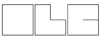
Figure 1. The domains $\Omega_{1}$, $\Omega_{2}$, and $\Omega_{3}$.

The corresponding problems (1.1) were discretized by the standard Taylor–Hood element on a uniform triangular grid to obtain a discrete anolog of this system (2.2) on the form

$${\mathcal{A}}_{\operatorname{\epsilon},h}\begin{pmatrix}u_{h}\\ p_{h}\end{pmatrix}=\begin{pmatrix}f_{h}\\ g_{h}\end{pmatrix}.$$

Here the parameter $h$ indicates the mesh size. We have computed the condition numbers of the operator ${\mathcal{B}}_{\operatorname{\epsilon},h}{\mathcal{A}}_{\operatorname{\epsilon},h}$ for different values of $\operatorname{\epsilon}$ and $h$ for the three domains. The operator ${\mathcal{B}}_{\operatorname{\epsilon},h}$ is given as the corresponding discrete version of (2.5), i.e., exact inverses of the discrete elliptic operators appearing in (2.5) are used. Hence, in the notation of [15] a canonical preconditioner is applied. The results are given in Table 1 below.

domain	$\operatorname{\epsilon}\backslash h$	$2^{-2}$	$2^{-3}$	$2^{-4}$	$2^{-5}$
$\quad\Omega_{1}$	1	14.3	15.3	18.5	22.0
	0.1	10.3	11.9	12.7	13.2
	0.01	6.2	6.7	8.0	9.9
$\quad\Omega_{2}$	1	17.1	17.2	17.1	17.1
	0.1	10.3	11.8	12.7	13.2
	0.01	6.1	6.7	8.0	9.9
$\quad\Omega_{3}$	1	13.2	13.4	13.5	13.6
	0.1	10.3	11.9	12.8	13.2
	0.01	6.1	6.7	8.1	9.9

Table 1. Condition numbers for the operators ${\mathcal{B}}_{\operatorname{\epsilon},h}{\mathcal{A}}_{\operatorname{\epsilon},h}$

These results indicate clearly that the condition numbers of the operators ${\mathcal{B}}_{\operatorname{\epsilon},h}{\mathcal{A}}_{\operatorname{\epsilon},h}$ are not dramatically effected by lack of convexity of the domains. Actually, we will show below that these condition numbers are indeed uniformly bounded both with respect to the perturbation parameter $\operatorname{\epsilon}$ and the discretization parameter $h$.

We will now return to a verification of the inf–sup condition (2.4) for general Lipschitz domains. The problem we encountered above in the nonconvex case is caused by the lack of regularity of the solution operator for Stokes problem on general Lipschitz domains. However, to establish (2.4) we are not restricted to such solution operators. It should be clear from the discussion above that if we can find any operator $S$ satisfying condition (3.4), then (2.4) will hold. A proper operator which satisfy these conditions is the Bogovskiĭ operator, see for example [11, section III.3], or [8, 12]. On a domain $\Omega$, which is star shaped with respect to an open ball $B$, this operator is explicitly given as an integral operator on the form

$$Sg(x)=\int_{\Omega}g(y)K(x-y,y)\,dy,\quad\text{where }K(z,y)=\frac{z}{|z|^{n}}\int_{|z|}^{\infty}\theta(y+r\frac{z}{|z|})r^{n-1}\,dr.$$

Here $\theta\in C_{0}^{\infty}(\mathbb{R}^{n})$ with

$$\operatorname{supp}\theta\subset B,\quad\text{and }\int_{\mathbb{R}^{n}}\theta(x)\,dx=1.$$

This operator is a right inverse of the divergence operator, and it has exactly the desired mapping properties given by (3.4), cf. [8, 12]. Furthermore, the definition of the right inverse $S$ can also be extended to general bounded Lipschitz domains, by using the fact that such domains can be written as a finite union of star shaped domains. The constructed operator will again satisfy the properties given by (3.4). We refer to [11, section III.3], [12, section 2], and [8, section 4.3] for more details. We can therefore conclude our discussion so far with the following theorem.

Theorem 3.1.

Assume that $\Omega$ is a bounded Lipshitz domain. Then the uniform inf–sup condition (2.4) holds.

4. Preconditioning the discrete coefficient operator

The purpose of this final section is to show discrete variants of Theorem 3.1 for various finite element discretizations of the problem (1.1). More precisely, we will consider finite element discretizations of the system (1.1) of the form:

Find $(u_{h},p_{h})\in V_{h}\times Q_{h}$ such that

(4.1) $$\begin{array}[]{rll}\langle u_{h},v\rangle+\operatorname{\epsilon}^{2}\langle Du_{h},Dv\rangle&+\,\langle p_{h},\operatorname{div}v\rangle&=\langle f,v\rangle,\quad v\in V_{h},\\ \langle\operatorname{div}u_{h},q\rangle&&=\langle g,q\rangle,\quad q\in Q_{h}.\end{array}$$

Here $V_{h}$ and $Q_{h}$ are finite element spaces such that $V_{h}\times Q_{h}\subset H_{0}^{1}(\Omega;\mathbb{R}^{n})\times L^{2}_{0}(\Omega)$, and $h$ is the discretization parameter. Alternatively, these problems can be written on the form

$${\mathcal{A}}_{\operatorname{\epsilon},h}\begin{pmatrix}u_{h}\\ p_{h}\end{pmatrix}=\begin{pmatrix}f_{h}\\ g_{h}\end{pmatrix},$$

where the coefficient operator ${\mathcal{A}}_{\operatorname{\epsilon},h}$ is acting on elements of $V_{h}\times Q_{h}$. In the examples below we will, for simplicity, only consider discretizations where the finite element space $V_{h}\times Q_{h}\subset X_{\operatorname{\epsilon}}$ for all $\operatorname{\epsilon}$ in the closed interval $[0,1]$. This implies that also the pressure space $Q_{h}$ is a subspace of $H^{1}$. The proper discrete uniform inf–sup conditions we shall establish will be of the form

(4.2) $$\sup_{v\in V_{h}}\frac{\langle\operatorname{div}v,q\rangle}{\|v\|_{L^{2}\cap\operatorname{\epsilon}H^{1}}}\geq\alpha\|q\|_{H^{1}+\operatorname{\epsilon}^{-1}L^{2},h},\quad q\in Q_{h},$$

where the positive constant $\alpha$ is independent of both $\operatorname{\epsilon}$ and $h$. Here the discrete norm $\|\cdot\|_{H^{1}+\operatorname{\epsilon}^{-1}L^{2},h}$ is defined as

$$\|q\|_{H^{1}+\operatorname{\epsilon}^{-1}L^{2},h}^{2}=\inf_{\begin{subarray}{c}q_{1},q_{2}\in Q_{h}\\ q=q_{1}+q_{2}\end{subarray}}(\|q_{1}\|_{H^{1}}^{2}+\operatorname{\epsilon}^{-2}\|q_{2}\|_{L^{2}}^{2}),\quad q\in Q_{h}.$$

The technique we will use to establish the discrete inf–sup condition (4.2) is in principle rather standard. We will just rely on the corresponding continuous condition (2.4) and a bounded projection operator into the velocity space $V_{h}$. The key property is that the projection operator $\varPi_{h}$ commutes properly with the divergence operator, cf. (4.4) below, and that it is uniformly bounded in the proper operator norm. Such projection operators are frequently referred to as Fortin operators.

We will restrict the discussion below to two key examples, the Mini element and the Taylor–Hood element. For both these examples we will construct interpolation operators $\varPi_{h}:L^{2}(\Omega;\mathbb{R}^{n})\to V_{h}$ which are uniformly bounded, with respect to $h$, in both $L^{2}$ and $H_{0}^{1}$. Therefore, these operators will be uniformly bounded operators in ${\mathcal{L}}((L^{2}\cap\operatorname{\epsilon}H_{0}^{1})(\Omega;\mathbb{R}^{n}))$, i.e., we have

(4.3) $$\|\varPi_{h}\|_{{\mathcal{L}}((L^{2}\cap\operatorname{\epsilon}H_{0}^{1})}\quad\text{is bounded independently of }\operatorname{\epsilon}\,\text{and }h.$$

It is easy to see that this is equivalent to the requirement that $\varPi_{h}$ is uniformly bounded with respect to $h$ in ${\mathcal{L}}(L^{2})$ and ${\mathcal{L}}(H_{0}^{1})$. Furthermore, the operators $\varPi_{h}$ will satisfy a commuting relation of the form

(4.4) $$\langle\operatorname{div}\varPi_{h}v,q\rangle=\langle\operatorname{div}v,q\rangle\quad v\in H_{0}^{1}(\Omega;\mathbb{R}^{n}),\,q\in Q_{h}.$$

As a consequence, the discrete uniform inf–sup condition (4.2) will follow from the corresponding condition (2.4) in the continuous case. We recall from Theorem 3.1 that (2.4) holds for any bounded Lipschitz domain, and without any convexity assumption, and as a consequence of the analysis below the discrete condition (4.2) will also hold without any convexity assumptions. The key ingredient in the analysis below is the construction of a uniformly bounded interpolation operator $\varPi_{h}$. In the case of the Mini element the construction we will present is rather standard, and resembles the presentation already done in [1], where this element was originally proposed (cf. also [5, Chapter VI]). However, for the Taylor–Hood element the direct construction of a bounded, commuting interpolation operator is not obvious. In fact, most of the stability proofs found in the literature for this discretization typically uses an alternative approach, cf. for example [5, Section VI.6] and the discussion given in the introduction of [10]. An exception is [10], where a projection satisfying (4.4) is constructed. However, this operator is not bounded in $L^{2}$. Below we propose a new construction of projection operators satisfying (4.4) by utilizing a technique for the Taylor–Hood method which is similar to the construction for Mini element presented below. The new projection operator will be bounded in both $L^{2}$ and $H^{1}$, and hence it satisfies (4.3). This analysis is restricted to quasi–uniform meshes in two space dimensions.

In the present case, the discrete inf–sup condition (4.2) will imply uniform stability of the discretization in the proper norms introduced above. As a consequence, we are able to derive preconditioners ${\mathcal{B}}_{\operatorname{\epsilon},h}$, such that the condition numbers of the corresponding operators ${\mathcal{B}}_{\operatorname{\epsilon},h}{\mathcal{A}}_{\operatorname{\epsilon},h}$ are bounded uniformly with respect to the perturbation parameter $\operatorname{\epsilon}$ and the discretization parameter $h$. The operator ${\mathcal{B}}_{\operatorname{\epsilon},h}$ can be taken as a block diagonal operator of the form (2.5), but where the elliptic operators are replaced by the corresponding discrete analogs. In fact, to obtain an efficient preconditioner the inverses of the elliptic operators which appear should be replaced by corresponding elliptic preconditioners, constructed for example by a standard multigrid procedure. We refer to [15], see in particular Section 5 of that paper, for a discussion on the relation between stability estimates and the construction of uniform preconditioners. In particular, the results for the Taylor–Hood method presented below explains the uniform behavior of the preconditioner ${\mathcal{B}}_{\operatorname{\epsilon},h}$ observed in the numerical experiment reported in Table 1 above.

4.1. The discrete inf–sup condition

The rest of the paper is devoted to the construction of proper interpolation operators $\varPi_{h}$ for the Mini element and the Taylor–Hood element, i.e, we will construct interpolation operators $\varPi_{h}:L^{2}(\Omega;\mathbb{R}^{n})\to V_{h}$ such that (4.3) and (4.4) holds. We will assume that the domain $\Omega$ is a polyhedral domain which is triangulated by a family of shape regular, simplicial meshes $\{{\mathcal{T}}_{h}\}$ indexed by decreasing values of the mesh parameter $h=\max_{T\in{\mathcal{T}}_{h}}h_{T}$. Here $h_{T}$ is the diameter of the simplex $T$. We recall that the mesh is shape regular if the there exist a positive constant $\gamma_{0}$ such that for all values of the mesh parameter $h$

$$h_{T}^{n}\leq\gamma_{0}|T|,\quad T\in T_{h}.$$

Here $|T|$ denotes the volume of $T$.

4.1.1. The Mini element

We recall that for this element the velocity space, $V_{h}$, consists of linear combinations of continuous piecewise linear vector fields and local bubbles. More precisely, $v\in V_{h}$ if and only if

$$v=v^{1}+\sum_{T\in{\mathcal{T}}_{h}}c_{T}b_{T},$$

where $v^{1}$ is a continuous piecewise linear vector field, $c_{T}\in\mathbb{R}^{n}$, and $b_{T}\in{\mathcal{P}}_{n+1}(T)$ is the bubble function with respect to $T$, i.e. the unique polynomial of degree $n+1$ which vanish on $\partial T$ and with $\int_{T}b_{T}\,dx=1$. The pressure space $Q_{h}$ is the standard space of continuous piecewise linear scalar fields.

In order to define the operator $\varPi_{h}$ we will utilize the fact that the space $V_{h}$ can be decomposed into two subspaces, $V_{h}^{b}$, consisting of all functions which are identical to zero on all element boundaries, i.e. $V_{h}^{b}$ is the span of the bubble functions, and $V_{h}^{1}$ consisting of continuous piecewise linear vector fields. Let $\varPi_{h}^{b}:L^{2}(\Omega;\mathbb{R}^{n})\to V_{h}^{b}$ be defined by,

$$\langle\varPi^{b}_{h}v,z\rangle=\langle v,z\rangle\qquad\forall z\in Z_{h},$$

where $Z_{h}$ denotes the space of piecewise constants vector fields. Clearly this uniquely determines $\varPi^{b}_{h}$. Furthermore, a scaling argument, utilizing equivalence of norms, shows that the local operators $\varPi^{b}_{h}$ are uniformly bounded, with respect to $h$, in $L^{2}(\Omega;\mathbb{R}^{n})$.

The operator $\varPi^{b}_{h}$ will satisfy property (4.4) since for all $v\in H^{1}_{0}(\Omega;\mathbb{R}^{n})$ and $q\in Q_{h}$, we have

(4.5) $$\langle\operatorname{div}\varPi_{h}^{b}v,q\rangle=-\langle\varPi_{h}^{b}v,\operatorname{grad}q\rangle=-\langle v,\operatorname{grad}q\rangle=\langle\operatorname{div}v,q\rangle,$$

where we have used that $\operatorname{grad}Q_{h}\subset Z_{h}$.

The desired operator $\varPi_{h}$ will be of the form

$$\varPi_{h}=\varPi_{h}^{b}(I-R_{h})+R_{h},$$

where $R_{h}:L^{2}(\Omega;\mathbb{R}^{n})\to V_{h}^{1}$ will be specified below. Note that

$$I-\varPi_{h}=(I-\varPi_{h}^{b})(I-R_{h}),$$

and therefore

$$\langle\operatorname{div}(I-\varPi_{h})v,q\rangle=\langle\operatorname{div}(I-\varPi^{b}_{h})(I-R_{h})v,q\rangle)=0$$

for all $q\in Q_{h}$. Hence, the operator $\varPi_{h}$ satisfies (4.4).

We will take $R_{h}$ to be the Clement interpolant onto piecewise linear vector fields, cf. [7]. Hence, in particular, the operator $R_{h}$ is local, it preserves constants, and it is stable in $L^{2}$ and $H_{0}^{1}$. More precisely, we have for any $T\in{\mathcal{T}}_{h}$ that

(4.6) $$\|(I-R_{h})v\|_{H^{j}(T)}\leq ch_{\Omega_{T}}^{k-j}\|v\|_{H^{k}(\Omega_{T})},\qquad 0\leq j\leq k\leq 1,$$

where the constant $c$ is independent of $h$ and $v$. Here $\Omega_{T}$ denote the macroelement consisting of $T$ and all elements $T^{\prime}\in{\mathcal{T}}_{h}$ such that $T\cap T^{\prime}\neq\emptyset$, and $h_{\Omega_{T}}=\max_{T\in{\mathcal{T}}_{h},T\subset\Omega_{h}}h_{T}$. It also follows from the shape regularity of the family $\{{\mathcal{T}}_{h}\}$ that the covering $\{\Omega_{T}\}_{T\in{\mathcal{T}}_{h}}$ has a bounded overlap. Therefore, it follows from (4.6) and the $L^{2}$ boundedness of $\varPi_{h}^{b}$ that $\varPi_{h}$ is uniformly bounded in ${\mathcal{L}}(L^{2}(\Omega;\mathbb{R}^{n}))$. Furthermore, by combining (4.6) with a standard inverse estimate for polynomials we have for any $T\in{\mathcal{T}}_{h}$ that

$$\|\varPi_{h}v\|_{H^{1}(T)} \leq\|\varPi_{h}^{b}(I-R_{h})v\|_{H^{1}(T)}+\|R_{h}v\|_{H^{1}(T)}$$

$$\leq c(h_{T}^{-1}\|\varPi_{h}^{b}(I-R_{h})v\|_{L^{2}(T)}+\|v\|_{H^{1}(T)})$$

$$\leq c(h_{T}^{-1}\|(I-R_{h})v\|_{L^{2}(T)}+\|v\|_{H^{1}(T)})$$

$$\leq c(h_{T}^{-1}h_{\Omega_{T}}+1)\|v\|_{H^{1}(\Omega_{T})}$$

$$\leq c\|v\|_{H^{1}(\Omega_{T})},$$

where we have used that $h_{T}^{-1}h_{\Omega_{T}}$ is uniformly bounded by shape regularity. This implies that $\varPi_{h}$ is uniformly bounded in ${\mathcal{L}}(H_{0}^{1}(\Omega;\mathbb{R}^{n}))$. We have therefore verified (4.3). Together with (4.4) this implies (4.2). In Table 2 below we present results for the Mini element which are completely parallel to results for the Taylor–Hood element presented in Table 1 above. As we can see, by comparing the results of the two tables, the effect of the different discretizations seems to minor, as long as the mesh is the same.

domain	$\operatorname{\epsilon}\backslash h$	$2^{-2}$	$2^{-3}$	$2^{-4}$	$2^{-5}$
$\quad\Omega_{1}$	1	26.6	24.7	25.7	27.0
	0.1	9.5	12.7	15.1	17.0
	0.01	3.4	4.0	5.7	9.2
$\quad\Omega_{2}$	1	27.0	20.8	19.2	18.6
	0.1	9.0	12.3	15.1	16.7
	0.01	3.4	4.0	5.5	8.3
$\quad\Omega_{3}$	1	15.8	17.3	17.8	17.9
	0.1	8.8	12.4	15.1	16.7
	0.01	3.4	4.0	5.5	8.3

Table 2. Condition numbers for the operators ${\mathcal{B}}_{\operatorname{\epsilon},h}{\mathcal{A}}_{\operatorname{\epsilon},h}$ discretized with the Mini element.

4.1.2. The Taylor–Hood element

Next we will consider the classical Taylor–Hood element. We will restrict the discussion to two space dimensions, and we will assume that the family of meshes $\{{\mathcal{T}}_{h}\}$ is quasi–uniform. More precisely, we assume that there is a mesh independent constant $\gamma_{1}>0$ such that

(4.7) $$h_{T}\geq\gamma_{1}\,h,\quad T\in{\mathcal{T}}_{h},$$

where we recall that $h=\max_{T}h_{T}$. For the Taylor–Hood element the velocity space, $V_{h}$, consists of continuous piecewise quadratic vector fields, and as for the Mini element above $Q_{h}$ is the standard space of continuous piecewise linear scalar fields. Note that if we have established the discrete inf–sup condition for a pair of spaces $(V_{h}^{-},Q_{h})$, where $V_{h}^{-}$ is a subspace of $V_{h}$, then this condition will also hold for the pair $(V_{h},Q_{h})$. This observation will be utilized here.

For technical reasons we will assume in the rest of this section that any $T\in{\mathcal{T}}_{h}$ has at most one edge in $\partial\Omega$. Such an assumption is frequently made for convenience when the Taylor–Hood element is analyzed, cf. for example [5, Proposition 6.1], since most approaches requires a special construction near the boundary. On the other hand, this assumption will not hold for many simple triangulations. Therefore, in Section 4.1.3 below we will refine our analysis, and, as a consequence, this assumption will be relaxed.

We let $V_{h}^{-}\subset V_{h}\subset H_{0}^{1}(\Omega;\mathbb{R}^{2})$ be the space of piecewise quadratic vector fields which has the property that on each edge of the mesh the normal components of elements in $V_{h}^{-}$ are linear. Each function $v$ in the space $V_{h}^{-}$ can be determined from its values at each interior vertex of the mesh, and of the mean value of the tangential component along each interior edge. In fact, in analogy with the discussion of the Mini element above, the space $V_{h}^{-}$ can be decomposed as $V_{h}^{-}=V_{h}^{1}\oplus V_{h}^{b}$. As above the space $V_{h}^{1}$ is the space of continuous piecewise linear vector fields, while the space $V_{h}^{b}$ in this case is spanned by quadratic “edge bubbles.” To define this space of bubbles we let

$$\Delta_{1}({\mathcal{T}}_{h})=\Delta_{1}^{i}({\mathcal{T}}_{h})\cup\Delta_{1}^{\partial}({\mathcal{T}}_{h})$$

be the set of the edges of the mesh ${\mathcal{T}}_{h}$, where $\Delta_{1}^{i}({\mathcal{T}}_{h})$ are the interior edges and $\Delta_{1}^{\partial}({\mathcal{T}}_{h})$ are the edges on the boundary of $\Omega$. Furthermore, if $T\in{\mathcal{T}}_{h}$ then $\Delta_{1}(T)$ are the set of edges of $T$, and $\Delta_{1}^{i}(T)=\Delta_{1}(T)\cap\Delta_{1}^{i}({\mathcal{T}})$.

For each $e\in\Delta_{1}({\mathcal{T}}_{h})$ we let $\Omega_{e}$ be the associated macroelement consisting of the union of all $T\in{\mathcal{T}}_{h}$ with $e\in\Delta_{1}(T)$. The scalar function $b_{e}$ is the unique continuous and piecewise quadratic function on $\Omega_{e}$ which vanish on the boundary of $\Omega_{e}$, and with $\int_{e}b_{e}\,ds=|e|$, where $|e|$ denotes the length of $e$. The space $V_{h}^{b}$ is defined as

$$V_{h}^{b}=\operatorname{span}\{b_{e}t_{e}\,|\,e\in\Delta_{1}^{i}({\mathcal{T}}_{h})\,\},$$

where $t_{e}$ is a tangent vector along $e$ with length $|e|$. Alternatively, if $x_{i}$ and $x_{j}$ are the vertices corresponding to the endpoints of $e$ then the vector field $\psi_{e}=b_{e}t_{e}$ is determined up to a sign as $\psi_{e}=6\lambda_{i}\lambda_{j}(x_{j}-x_{i})$, where $\{\lambda_{i}\}$ are the piecewise linear functions corresponding to the barycentric coordinates, i.e., $\lambda_{i}(x_{k})=\delta_{i,k}$ for all vertices $x_{k}$. In particular,

$$\int_{e}\psi_{e}\cdot(x_{j}-x_{i})\,ds=6\int_{e}\lambda_{i}\lambda_{j}\,ds|e|^{2}=|e|^{3}.$$

As above the desired interpolation operator $\varPi_{h}$ will be of the form

$$\varPi_{h}=\varPi_{h}^{b}(I-R_{h})+R_{h},$$

where $R_{h}:L^{2}(\Omega;\mathbb{R}^{3})\to V_{h}^{1}$ is the same Clement operator as above, and where $\varPi_{h}^{b}:L^{2}(\Omega;\mathbb{R}^{n})\to V_{h}^{b}$ needs to be specified. In fact, to perform a construction similar to the one we did for the Mini element it will be sufficient to construct $\varPi_{h}^{b}$ such that it is $L^{2}$–stable, and satisfies the commuting relation (4.5).

We will need to separate the triangles which have an edge on the boundary of $\Omega$ from the interior triangles. With this purpose we define

$${\mathcal{T}}_{h}^{\partial}=\{T\in{\mathcal{T}}_{h}\,|\,T\cap\partial\Omega\in\Delta_{1}^{\partial}({\mathcal{T}}_{h})\,\}\quad\text{and}\quad{\mathcal{T}}_{h}^{i}={\mathcal{T}}_{h}\setminus{\mathcal{T}}_{h}^{\partial}.$$

In order to define the operator $\varPi_{h}^{b}$ we introduce $Z_{h}$ as the lowest order Nedelec space with respect to the mesh ${\mathcal{T}}_{h}$. Hence, if $z\in Z_{h}$ then on any $T\in{\mathcal{T}}_{h}$, $z$ is a linear vector field such that $z(x)\cdot x$ is also linear. Furthermore, for each $e\in\Delta_{1}({\mathcal{T}}_{h})$ the tangential component of $z$ is continuous. As a consequence, $Z_{h}\subset H(\operatorname{curl};\Omega)$ where the operator $\operatorname{curl}$ denotes the two dimensional analog of the curl–operator given by

$$\operatorname{curl}z=\operatorname{curl}(z_{1},z_{2})=\partial_{x_{2}}z_{1}-\partial_{x_{1}}z_{2}.$$

It is well known that the proper degrees of freedom for the space $Z_{h}$ is the mean value of the tangential components of $v$, $v\cdot t$, with respect to each edge in $\Delta_{1}({\mathcal{T}}_{h})$. Furthermore, we let

$$Z_{h}^{0}=\{z\in Z_{h}\,|\,\int_{\partial T}z\cdot t\,ds=0,\,T\in{\mathcal{T}}_{h}^{\partial}\,\}.$$

Alternatively, the elements of $Z_{h}^{0}$ are those vector fields in $Z_{h}$ with the property that $\operatorname{curl}z|_{T}=0$ if $T\in{\mathcal{T}}_{h}^{\partial}$, i.e., $z$ is a constant vector field on $T$ for $T\in{\mathcal{T}}_{h}^{\partial}$. It is a key observation that the mesh assumption given above, that any $T\in{\mathcal{T}}_{h}$ intersects $\partial\Omega$ in at most one edge, implies that the spaces $V_{h}^{b}$ and $Z_{h}^{0}$ have the same dimension. Furthermore, we note that $\operatorname{grad}q\in Z_{h}^{0}$ for any $q\in Q_{h}$.

For each $e\in\Delta_{1}({\mathcal{T}}_{h})$ let $\phi_{e}\in Z_{h}$ be the basis function corresponding to the Whitney form, i.e., $\phi_{e}$ satisfies

$$\int_{e}(\phi_{e}\cdot t_{e})\,ds=|e|,\quad\text{and }\int_{e^{\prime}}(\phi_{e}\cdot t_{e^{\prime}})\,ds=0,\quad e^{\prime}\neq e,$$

where, as above, $t_{e}$ is a tangent vector of length $e$. Hence, if $e=(x_{i},x_{j})$ then the vector field $\phi_{e}$ can be expressed in barycentric coordinates as

$$\phi_{e}=\lambda_{i}\operatorname{grad}\lambda_{j}-\lambda_{j}\operatorname{grad}\lambda_{i}.$$

Any $z\in Z_{h}^{0}$ can be written uniquely on the form

$$z=\sum_{e\in\Delta_{1}^{i}({\mathcal{T}}_{h})}a_{e}\phi_{e}+\sum_{e\in\Delta_{1}^{\partial}({\mathcal{T}}_{h})}c_{e}\phi_{e},$$

where the coefficients $a_{e}$ corresponding to interior edges can be chosen arbitrarily, but where the coefficients $c_{e}$ for each boundary edge should be chosen such that $\operatorname{curl}z=0$ on the associated triangle in ${\mathcal{T}}_{h}^{\partial}$. We note that there is a natural mapping $\Phi_{h}$ between the spaces $V_{h}^{b}$ and $Z_{h}^{0}$ given by $\Phi_{h}(\psi_{e})=\phi_{e}$ for all interior edges, or alternatively,

(4.8) $$\int_{e}\Phi_{h}(v)\cdot t_{e}\,ds=|e|^{-2}\,\int_{e}v\cdot t_{e}\,ds,\quad e\in\Delta_{1}^{i}({\mathcal{T}}_{h}).$$

Below, we will use $V_{h}^{b}(T)$ and $Z_{h}^{0}(T)$ to denote the restriction of the spaces $V_{h}^{b}$ and $Z_{h}^{0}$ to a single element $T$, and $\Phi_{T}$ will denote the corresponding restriction of the map $\Phi_{h}$.

We will define the operator $\varPi_{h}^{b}:L^{2}(\Omega;\mathbb{R}^{n})\to V_{h}^{b}$ by,

(4.9) $$\langle\varPi^{b}_{h}u,z\rangle=\langle u,z\rangle\qquad\forall z\in Z_{h}^{0}.$$

To show that this operator is well–defined the following general formula for integration of products of barycentric coordinates over a triangle $T$ will be useful (cf. for example [14, Section 2.13])

(4.10) $$\int_{T}\lambda_{1}^{\alpha_{1}}\lambda_{2}^{\alpha_{2}}\lambda_{3}^{\alpha_{3}}\,dx=\frac{2\alpha!}{(2+|\alpha|)!}|T|,$$

where $\alpha!=\alpha_{1}!\alpha_{2}!\alpha_{3}!$, $|\alpha|=\sum_{i}\alpha_{i}$ and $|T|$ is the area of $T$.

Lemma 4.1.

Let $T\in{\mathcal{T}}_{h}^{i}$ with edges $e_{1},e_{2},e_{3}$. For any $v\in V_{h}^{b}(T)$ we have

$$\int_{T}v\cdot\Phi_{T}(v)\,dx\geq\frac{1}{5}|a|^{2}|T|,$$

where $\Phi_{T}=\Phi_{h}|_{T}$, $v=\sum_{i}a_{i}\psi_{e_{i}}$ and $|a|^{2}=\sum_{i}a_{i}^{2}$.

Proof.

A direct computation gives

$$\int_{T}v\cdot\Phi_{T}(v)\,dx=\sum_{i=1}^{3}\sum_{j=1}^{3}a_{i}a_{j}\,\int_{T}\psi_{e_{i}}\cdot\phi_{e_{j}}\,dx=\sum_{i=1}^{3}\sum_{j=1}^{3}a_{i}a_{j}\,\int_{T}b_{e_{i}}\phi_{e_{j}}\cdot t_{e_{i}}\,dx=a^{T}Ma,$$

where the $3\times 3$ matrix $M$ is given by

$$M=\{M_{i,j}\}_{i,j=1}^{3}=\{\int_{T}\psi_{i}\cdot\phi_{e_{j}}\,dx\}_{i,j=1}^{3}\{\int_{T}b_{e_{i}}\phi_{e_{j}}\cdot t_{e_{i}}\,dx\}_{i,j=1}^{3},$$

The desired result will follow from the diagonal dominance of this matrix.

Let $x_{j}$ be the vertex opposite $e_{j}$, and let $\lambda_{j}$ be the corresponding barycentric coordinate on $T$. Then the first diagonal element $M_{1,1}$ of the matrix $M$ is given by

$$M_{1,1}=6\,\int_{T}\lambda_{2}\lambda_{3}(\lambda_{2}\operatorname{grad}\lambda_{3}-\lambda_{3}\operatorname{grad}\lambda_{2})(x_{3}-x_{2})\,dx=6\,\int_{T}(\lambda_{2}^{2}\lambda_{3}+\lambda_{2}\lambda_{3}^{2})\,dx=2|T|/5,$$

where we have used formula (4.10) in the final step. Actually, from this formula we derive that all the diagonal elements are given by $M_{i,i}=2|T|/5$, and similar calculations for the off–diagonal elements gives $|M_{i,j}|=|T|/10$. In addition, the matrix $M$ is symmetric. The matrix $M$ is therefore strictly diagonally dominant, and by the Gershgorin circle theorem all eigenvalues are bounded below by $|T|/5$. By combining this with the fact that $M$ is symmetric we conclude that $a^{T}Ma\geq|a|^{2}|T|/5$, and this is the desired bound. ∎

The next lemma is a variant of the result above for $T\in{\mathcal{T}}_{h}^{\partial}$.

Lemma 4.2.

Let $T\in{\mathcal{T}}_{h}^{\partial}$ with interior edges $e_{1},e_{2}$, and where $e_{3}$ is the edge on the boundary. For any $v\in V_{h}^{b}(T)$ we have

$$\int_{T}v\cdot\Phi_{T}(v)\,dx\geq\frac{1}{2}|a|^{2}|T|,$$

where $v=a_{1}\psi_{e_{1}}+a_{2}\psi_{e_{2}}$ and $|a|^{2}=a_{1}^{2}+a_{2}^{2}$.

Proof.

Let $v=a_{1}\psi_{e_{1}}+a_{2}\psi_{e_{2}}=6a_{1}\lambda_{2}\lambda_{3}(x_{3}-x_{2})+6a_{2}\lambda_{1}\lambda_{3}(x_{3}-x_{1})$. It is a key observation that in this case $\Phi_{T}(v)$ is simply given as $\Phi(v)=-a_{1}\operatorname{grad}\lambda_{2}-a_{2}\operatorname{grad}\lambda_{1}$. Since $\operatorname{grad}\lambda_{i}\cdot t_{e_{i}}\equiv 0$ we therefore obtain from (4.10) that

$$\int_{T}v\cdot\Phi_{T}(v)\,dx =6a_{1}^{2}\int_{T}\lambda_{2}\lambda_{3}\operatorname{grad}\lambda_{2}\cdot(x_{2}-x_{3})\,dx+6a_{2}^{2}\int_{T}\lambda_{1}\lambda_{3}\operatorname{grad}\lambda_{1}\cdot(x_{1}-x_{3})\,dx$$

$$=6a_{1}^{2}\int_{T}\lambda_{2}\lambda_{3}\,dx+6a_{2}^{2}\int_{T}\lambda_{1}\lambda_{3}\,dx=\frac{1}{2}|a|^{2}|T|.$$

This completes the proof. ∎

Lemma 4.3.

There is a positive constant $c_{0}$, independent of $h$, such that for each $v\in V_{h}^{b}$

$$\sup_{z\in Z_{h}^{0}}\frac{\langle v,z\rangle}{\|z\|_{L^{2}(\Omega)}}\geq c_{0}\|v\|_{L^{2}(\Omega)}.$$

Proof.

Let $v\in V_{h}^{b}$ be given, i.e., $v=\sum_{e\in\Delta_{1}^{i}({\mathcal{T}}_{h})}a_{e}\psi_{e}$. We simply choose the corresponding $z=\Phi_{h}(v)=\sum_{e\in\Delta_{1}^{i}({\mathcal{T}}_{h})}a_{e}\phi_{e}+\sum_{e\in\Delta_{1}^{\partial}({\mathcal{T}}_{h})}c_{e}\phi_{e}\in Z_{h}^{0}$. It follows from scaling and shape regularity that the two norms of $z$, given by

(4.11) $$\|z\|_{L^{2}(\Omega)}\quad\text{and}\quad(\sum_{T\in{\mathcal{T}}_{h}}\sum_{e\in\Delta_{1}^{i}(T)}a_{e}^{2})^{1/2}$$

are equivalent uniformly in $h$. Correspondingly, the two norms

(4.12) $$\|v\|_{L^{2}(\Omega)}\quad\text{and}\quad(\sum_{T\in{\mathcal{T}}_{h}}|T|^{2}\sum_{e\in\Delta_{1}^{i}(T)}a_{e}^{2})^{1/2}$$

are uniformly equivalent. As a consequence of these properties, combined with Lemmas 4.1 and 4.2, we obtain

$$\langle v,\Phi_{h}(v)\rangle=\sum_{T\in{\mathcal{T}}_{h}}\int_{T}\Phi_{T}(v)\cdot v\,dx\geq\frac{1}{5}\sum_{T\in{\mathcal{T}}_{h}}|T|\sum_{e\in\Delta_{1}^{i}(T)}a_{e}^{2}\geq c_{0}\|\Phi_{h}(v)\|_{L^{2}(\Omega)}\,\|v\|_{L^{2}(\Omega)}.$$

where $c_{0}>0$ is independent of $h$. This completes the proof. ∎

It is a direct consequence of Lemma 4.3 that the operators $\varPi_{h}^{b}$ are uniformly bounded in ${\mathcal{L}}(L^{2}(\Omega;\mathbb{R}^{2}))$. In fact, the associated operator norm is bounded by $c_{0}^{-1}$. Note that in contrast to the situation for the Mini element, the operator $\varPi_{h}^{b}$ is not local in this case. However, if the mesh is quasi–uniform we obtain from (4.7) that

(4.13) $$\|\varPi_{h}^{b}u\|_{H^{1}(\Omega)}\leq c\big{(}\sum_{T\in{\mathcal{T}}_{h}}h_{T}^{-2}\|\varPi_{h}^{b}u\|_{L^{2}(T)}^{2}\big{)}^{1/2}\leq c\gamma_{1}^{-1}h^{-1}\|\varPi_{h}^{b}u\|_{L^{2}(\Omega)}.$$

As a further consequence we now obtain.

Theorem 4.4.

The operator $\varPi_{h}$ satisfies properties (4.3) and (4.4).

Proof.

To show that the operator $\varPi_{h}$ fulfills the condition (4.4), it is enough to show that the operator $\varPi_{h}^{b}$ satisfies the corresponding condition (4.5). However, since $\operatorname{grad}Q_{h}\subset Z_{h}^{0}$ this follows exactly as before, since

$$\langle\operatorname{div}\varPi_{h}^{b}v,q\rangle=-\langle\varPi_{h}^{b}v,\operatorname{grad}q\rangle=-\langle v,\operatorname{grad}q\rangle=\langle\operatorname{div}v,q\rangle.$$

Furthermore, to show (4.3) it is enough to show that $\varPi_{h}$ is uniformly bounded with respect to $h$ in both ${\mathcal{L}}(L^{2}(\Omega;\mathbb{R}^{2}))$ and ${\mathcal{L}}(H_{0}^{1}(\Omega;\mathbb{R}^{2}))$. However, the $L^{2}$–result follows from the corresponding bounds for the operators $\varPi_{h}^{b}$ and $R_{h}$. Finally, by combining (4.6), (4.13) and the boundedness of $\varPi_{h}^{b}$ in $L^{2}$ we obtain

$$\|\varPi_{h}v\|_{H^{1}(\Omega)} \leq\|\varPi_{h}^{b}(I-R_{h})v\|_{H^{1}(\Omega)}+\|R_{h}v\|_{H^{1}(\Omega)}$$

$$\leq c(h^{-1}\|\varPi_{h}^{b}(I-R_{h})v\|_{L^{2}(\Omega)}+\|v\|_{H^{1}(\Omega)})$$

$$\leq c(c_{0}^{-1}h^{-1}\|(I-R_{h})v\|_{L^{2}(\Omega)}+\|v\|_{H^{1}(\Omega)})$$

$$\leq c\|v\|_{H^{1}(\Omega)},$$

and this is the desired uniform bound in ${\mathcal{L}}(H_{0}^{1}(\Omega;\mathbb{R}^{2}))$. ∎

4.1.3. More general triangulations

The analysis of the Taylor–Hood method given above leans havily on the assumption that there are no triangles in ${\mathcal{T}}_{h}$ with more than one edge on the boundary of $\Omega$. This assumption simplifies the analysis, but it is not necessary. The purpose of this section is to relax this assumption.

We let ${\mathcal{T}}_{h}^{\partial,1}$ and ${\mathcal{T}}_{h}^{\partial,2}$ denote the subset of triangles in ${\mathcal{T}}_{h}$ with one or two edges in $\partial\Omega$, respectively. We let ${\mathcal{T}}_{h}^{\partial}={\mathcal{T}}_{h}^{\partial,1}\cup{\mathcal{T}}_{h}^{\partial,2}$ be the set of all boundary triangles, and as before ${\mathcal{T}}_{h}^{i}={\mathcal{T}}_{h}\setminus{\mathcal{T}}_{h}^{\partial}$. We note that $T\in{\mathcal{T}}_{h}^{\partial,2}$ then there is a unique associated triangle $T^{-}\in{\mathcal{T}}_{h}$ such that $T\cap T^{-}\in\Delta_{1}^{i}({\mathcal{T}}_{h})$. We will denote this interior edge associated any $T\in{\mathcal{T}}_{h}^{\partial,2}$ by $e_{T}$, and we will use $T^{*}$ to denote the macroelement defined by the two triangles $T$ and $T^{-}$. The set of all interior edges of the form $e_{T},\,T\in{\mathcal{T}}_{h}^{\partial,2}$, will be denoted $\Delta_{1}^{i,2}({\mathcal{T}}_{h})$, while $\Delta_{1}^{i,1}({\mathcal{T}}_{h})=\Delta_{1}^{i}({\mathcal{T}}_{h})\setminus\Delta_{1}^{i,2}({\mathcal{T}}_{h})$. Throughout this section we will assume that all the triangles of the form $T^{-}$ are interior triangles, i.e.,

$$T^{-}\in{\mathcal{T}}_{h}^{i}\quad\text{for all }T\in{\mathcal{T}}_{h}^{\partial,2}.$$

The interpolation operators $\varPi_{h}$ and $\varPi_{h}^{b}$ will be defined as above, with the only exception that the definition of the bubble space $V_{h}^{b}$ is changed slightly in the neighborhood of the edges in $\Delta_{1}^{i,2}({\mathcal{T}}_{h})$. We note that the result of Lemma 4.2 still holds if $T\in{\mathcal{T}}_{h}^{\partial,1}$. To establish the result of Lemma 4.3, and as a consequence Theorem 4.4, in the present case we basically need an anolog of Lemma 4.2 for triangles $T\in{\mathcal{T}}_{h}^{\partial,2}$. More precisely, we need to modify the definition of the map $\Phi_{h}$, used in proof of Lemma 4.3, to the present case. Actually, the map $\Phi_{h}$ will not be defined locally on the triangles $T\in{\mathcal{T}}_{h}^{\partial,2}$, but rather on the corresponding macroelement $T^{*}$. As in the previous section the space $Z_{h}^{0}$ is taken to be the subspace of the Nedelec space $Z_{h}$ such that $z\in Z_{h}^{0}$ is constant on the triangles in ${\mathcal{T}}_{h}^{\partial}$. To be able to define the interpolation operator $\varPi_{h}^{b}$, mapping into the bubble space, by (4.9), the two spaces $V_{h}^{b}$ and $Z_{h}^{0}$ must be balanced. In particular, they should have the same dimension. However, in the present case the dimension of the space $Z_{h}^{0}$ is not the same as the number of interior edges. To see this just consider the restriction $Z_{h}^{0}(T^{*})$ of $Z_{h}^{0}$ to a macroelement macroelement $T^{*}$, cf. Figure 2 below. The dimension of the space $Z_{h}^{0}(T^{*})$ is four, while there are only three interior edges, namely the three edges of $T^{-}$. To compensate for this we will extend the space of bubble functions $V_{h}^{b}$, by including also “normal bubbles” on the edges $e_{T},\,T\in{\mathcal{T}}_{h}^{\partial,2}$.

In the present case we define the space $V_{h}^{b}\subset V_{h}$ by

$$V_{h}^{b}=\operatorname{span}(\{\,b_{e}t_{e}\,|\,e\in\Delta_{1}^{i}({\mathcal{T}}_{h})\,\}\cup\{\,b_{e}n_{e}\,|\,e\in\Delta_{1}^{i,2}({\mathcal{T}}_{h})\,\}).$$

Here $t_{e}$ and $n_{e}$ are tangent and normal vectors to the edge $e$ with length $|e|$. With this definition the space $V_{h}^{b}$ has the same dimension as $Z_{h}^{0}$. Furthermore, the map $\Phi_{h}:V_{h}^{b}\to Z_{h}^{0}$ will be defined to satisfy property (4.8) for all edges in $\Delta_{1}^{i,1}({\mathcal{T}}_{h})$. Note that this specifies $\Phi_{h}$ on all triangles in ${\mathcal{T}}_{h}$, except for the ones that belongs to the macroelements $T^{*}$, $T\in{\mathcal{T}}_{h}^{\partial,2}$. To complete the definition of $\Phi_{h}$ we need to specify its restriction to each macroelement $T^{*}$.

Consider a macroelement $T^{*}$ of the form given in Figure 2.

Figure 2. The macroelement $T^{*}$.

Here the edge $e_{T}$ has endpoints denoted by $x_{1}$ and $x_{2}$, the third boundary vertex of $T^{*}$ is $x_{0}$, while the single interior vertex of $T^{*}$ is $x_{3}$. We will use $e_{i}$ to denote the edge opposite $x_{i},\,i=1,2$, of the triangle $T$, while $e_{i}^{-}$ are the corresponding edges of the triangle $T^{-}$. We let $\Phi_{T}:V_{h}^{b}(T^{*})\to Z_{h}^{0}(T^{*})$ be the restriction of $\Phi_{h}$ to $T^{*}$. To be compatible with the definition of $\Phi_{h}$ outside the macroelements $T^{*}$ the map $\Phi_{T}$ has to satisfy condition (4.8) on the edges $e_{i}^{-}$, i.e.,

(4.14) $$\int_{e_{i}^{-}}\Phi_{T}(v)\cdot t_{e_{i}^{-}}\,ds=|e_{i}^{-}|^{-2}\,\int_{e_{i}^{-}}v\cdot t_{e_{i}^{-}}\,ds,\quad i=1,2,$$

where $t_{e_{i}^{-}}$ is a vector tangential to $e_{i}^{-}$. As a basis for the space $Z_{h}^{0}(T^{*})$ we will use the functions

$$\phi_{i}^{-}=\lambda_{i}\operatorname{grad}\lambda_{3}-\lambda_{3}\operatorname{grad}\lambda_{i},\quad i=1,2,$$

with support only in $T^{-}$, combined with the two functions $\phi_{i}$ given by

$$\phi_{i}=\left\{\begin{array}[]{cc}\operatorname{grad}\lambda_{i}&\text{on }T,\\ (-1)^{i}\phi_{T},&\text{on }T^{-},\end{array}\right.$$

for $i=1,2$, where $\phi_{T}=\lambda_{1}\operatorname{grad}\lambda_{2}-\lambda_{2}\operatorname{grad}\lambda_{1}$ corresponds to the Whitney form associated the edge $e_{T}=(x_{1},x_{2})$. The functions $\phi_{i},\phi_{i}^{-}$ for $i=1,2$ spans the space $Z_{h}^{0}(T^{*})$.

We will define two basis functions $\psi_{i}$ of $V_{h}^{b}$ as a multiple of the scalar bubble function $b_{e_{T}}$, namely,

(4.15) $$\psi_{i}=b_{e_{T}}w_{i}=6\lambda_{1}\lambda_{2}w_{i}\quad i=1,2,$$

where the vectors $w_{i}$ will be chosen below. Furthermore, the functions $\psi_{i}^{-}$, are given as

$$\psi_{i}^{-}=6\lambda_{i}\lambda_{3}(x_{3}-x_{i})+\beta(-1)^{i}\lambda_{1}\lambda_{2}(x_{2}-x_{1}),\quad i=1,2,$$

where $\beta=6|T^{-}|/(5|T|+4|T^{-}|)$. We note that $0<\beta<3/2$.

The functions $\psi_{i},\psi_{i}^{-}$ for $i=1,2$ span the space $V_{h}^{b}(T^{*})$, and we define $\Phi_{T}(\psi_{i})=\phi_{i}$ and $\Phi_{T}(\psi_{i}^{-})=\phi_{i}^{-}$. A map of this form will satisfy the compatibility condition (4.14) by construction. The motivation for the choice of the constant $\beta$ is that we obtain

(4.16) $$\int_{T^{*}}\psi_{i}^{-}\cdot\phi_{j}\,dx=0,\quad i,j=1,2.$$

Lemma 4.5.

The orthogonality conditions (4.16) hold.

Proof.

The identities (4.16) can be verified by formula (4.10). For example

$$\int_{T^{*}}\psi_{1}^{-}\cdot\phi_{1}\,dx =-\beta\int_{T}\lambda_{1}\lambda_{2}\operatorname{grad}\lambda_{1}\cdot(x_{2}-x_{1})\,dx$$

$$-\int_{T^{-}}(\lambda_{1}\operatorname{grad}\lambda_{2}-\lambda_{2}\operatorname{grad}\lambda_{1})\cdot(6\lambda_{1}\lambda_{3}(x_{3}-x_{1})-\beta\lambda_{1}\lambda_{2}(x_{2}-x_{1}))\,dx$$

$$=\beta\int_{T}\lambda_{1}\lambda_{2}\,dx-\int_{T^{-}}(6\lambda_{1}\lambda_{2}\lambda_{3}-\beta(\lambda_{1}^{2}\lambda_{2}+\lambda_{1}\lambda_{2}^{2}))\,dx$$

$$=(-6|T^{-}|+\beta(5|T|+4|T^{-}|)/60=0.$$

Furthermore, it is easy to check that

$$\int_{T^{*}}\psi_{1}^{-}\cdot\phi_{2}\,dx=-\int_{T^{*}}\psi_{1}^{-}\cdot\phi_{1}\,dx,$$

and as a consequence $\int_{T^{*}}\psi_{1}^{-}\cdot\phi_{2}\,dx=0$. Similar computations can be done for the integrals involving $\psi_{2}^{-}$. ∎

We can also verify, again using formula (4.10), that the $2\times 2$ matrix $M^{-}=\{M^{-}_{i,j}\}_{i,j=1,2}=\{\int_{T^{-}}\psi_{i}^{-}\cdot\phi_{j}^{-}\}_{i,j=1,2}$ is given by

$$M^{-}=|T^{-}|\begin{pmatrix}(24-\beta)/60&(6+\beta)/60\\ (6+\beta)/60&(24-\beta)/60\end{pmatrix}.$$

For $0<\beta<3/2$ this symmetric matrix is strictly diagonally dominant with both eigenvalues greater than $|T^{-}|/4$.

Finally, we need to investigate the $2\times 2$ matrix $M=\{M_{i,j}\}_{i,j=1,2}=\{\int_{T^{*}}\psi_{i}\cdot\phi_{j}\}_{i,j=1,2}$. However, first we need to define the functions $\psi_{i}=\Phi_{T}(\phi_{i})$ precisely by specifying the vectors $w_{i}$ in (4.15). We let

$$\psi_{1}=6\gamma\lambda_{1}\lambda_{2}(x_{3}-x_{2}),\quad\text{and }\psi_{2}=6\gamma^{-1}\lambda_{1}\lambda_{2}(x_{3}-x_{1}),$$

where the positive constant $\gamma$ will be chosen below.

Assume for a moment that $T^{*}$ is a parallelogram. Then $x_{3}-x_{1}=x_{2}-x_{0}$ and $x_{3}-x_{2}=x_{1}-x_{0}$, and therefore we would have easy computable representations of the functions $\psi_{i}$ on both $T$ and $T^{-}$. In general, we introduce a new point $\hat{x}_{0}\in\mathbb{R}^{2}$, depending on $T^{-}$, with the property that $\hat{x}_{0},x_{1},x_{2},x_{3}$ corresponds to the corners of a parallelogram, cf. Figure 3.

Figure 3. The macroelement $T^{*}$ and the associated parallelogram.

More precisely,

$$\hat{x}_{0}=x_{1}-(x_{3}-x_{2})=x_{1}+x_{2}-x_{3}.$$

Let $\{\hat{\lambda}_{i}\}_{i=0}^{2}$ be the barycentric coordinates with respect to the triangle $T$, extended to linear functions on all of $\mathbb{R}^{2}$. Then $\hat{\lambda}_{1}(x_{3})+\hat{\lambda}_{2}(x_{3})>1$ and

$$\hat{\lambda}_{1}(\hat{x}_{0})+\hat{\lambda}_{2}(\hat{x}_{0})=2-\hat{\lambda}_{1}(x_{3})+\hat{\lambda}_{2}(x_{3})<1.$$

In fact, it is a consequence of shape regularity that there is a constant $\alpha>0$, independent of $h$ and the choice of $T\in{\mathcal{T}}_{h}^{\partial,2}$, such that

(4.17) $$\hat{\lambda}_{1}(\hat{x}_{0})+\hat{\lambda}_{2}(\hat{x}_{0})\leq 1-\alpha.$$

If we compute the matrix $\{\int_{T}\psi_{i}\cdot\phi_{j}\,dx\}$ we obtain

$$\{\int_{T}\psi_{i}\cdot\phi_{j}\,dx\}_{i,j=1,2}=\frac{|T|}{2}\begin{pmatrix}\gamma(1-\hat{\lambda}_{1}(\hat{x}_{0}))&-\gamma\hat{\lambda}_{2}(\hat{x}_{0})\\ -\gamma^{-1}\hat{\lambda}_{1}(\hat{x}_{0})&\gamma^{-1}(1-\hat{\lambda}_{2}(\hat{x}_{0}))\end{pmatrix}.$$

To control the full matrix $M$ we also need to consider the contributions from the triangle $T^{-}$. A straightforward computation, using formula (4.10), shows that the matrix $\{\int_{T^{-}}\psi_{i}\cdot\phi_{j}\}$ is given by

$$\{\int_{T^{-}}\psi_{i}\cdot\phi_{j}\,dx\}_{i,j=1,2}=\frac{|T^{-}|}{5}\begin{pmatrix}\gamma&-\gamma\\ -\gamma^{-1}&\gamma^{-1}\end{pmatrix}.$$

We will utilize the constant $\gamma$ to obtain a symmetric matrix $M$. We define

$$\gamma=\sqrt{\frac{2|T^{-}|+5|T|\hat{\lambda}_{1}(\hat{x}_{0})}{2|T^{-}|+5|T|\hat{\lambda}_{2}(\hat{x}_{0})}}.$$

This choice of $\gamma$ is motivated by the desired identity

$$\gamma(\frac{|T|}{2}\hat{\lambda}_{2}(\hat{x}_{0})+\frac{|T^{-}|}{5})=\gamma^{-1}(\frac{|T|}{2}\hat{\lambda}_{1}(\hat{x}_{0})+\frac{|T^{-}|}{5}),$$

which can be seen to hold, and therefore the matrix $M$ is symmetric. Furthermore, we note that

$$\gamma,\gamma^{-1}\leq\sqrt{1+\frac{5|T|}{2|T^{-}|}}.$$

Therefore, it is a consequence of shape regularity that the positive constant $\gamma$ is bounded from above and below, independently of $h$ and the choice of $T\in{\mathcal{T}}_{h}^{\partial,2}$.

Lemma 4.6.

The matrix $M$ defined above is symmetric and positive definite with both eigenvalues bounded below by $c_{1}|T|$, where $c_{1}=\alpha\min(\gamma,\gamma^{-1})/2$.

Proof.

It follows from the calculations above that

$$M=\begin{pmatrix}\gamma(\frac{|T|}{2}(1-\hat{\lambda}_{1}(\hat{x}_{0}))+\frac{|T^{-}|}{5})&-\gamma(\frac{|T|}{2}\hat{\lambda}_{2}(\hat{x}_{0})+\frac{|T^{-}|}{5})\\ -\gamma^{-1}(\frac{|T|}{2}\hat{\lambda}_{1}(\hat{x}_{0})+\frac{|T^{-}|}{5})&\gamma^{-1}(\frac{|T|}{2}(1-\hat{\lambda}_{2}(\hat{x}_{0}))+\frac{|T^{-}|}{5})\end{pmatrix}.$$

Since $\hat{\lambda}_{1}(\hat{x}_{0})+\hat{\lambda}_{2}(\hat{x}_{0})\leq 1-\alpha$ it follows from Gershgorin circle theorem that both eigenvalues of $M$ are bounded below by $\frac{\alpha|T|}{2}\min(\gamma,\gamma^{-1})$. ∎

We now have the following result.

Lemma 4.7.

The conclusion of Lemma 4.3 holds in the present case.

Proof.

Let $v\in V_{h}^{b}$ be given. We first consider the situation on each macroelement $T^{*}$. If $v=\sum_{i}(a_{i}^{+}\psi_{i}+a_{i}^{-}\psi_{i}^{-})\in V_{h}^{b}(T^{*})$ then we write $v=v^{-}+v^{+}$, where $v^{-}=\sum_{i}a_{i}^{-}\psi_{i}^{-}$. Observe that Lemma 4.6, together with the orthogonality property (4.16), implies that

$$\int_{T^{*}}v\cdot\Phi_{T}(v^{+})\,dx=\int_{T^{*}}v^{+}\cdot\Phi_{T}(v^{+})\,dx\geq c_{1}|T||a^{+}|^{2}.$$

Similarly, we have from the property of the matrix $M^{-}$, the norm equivalences expressed by (4.11) and (4.12), and shape regularity that

$$\int_{T^{-}}v\cdot\Phi_{T}(v^{-})\,dx \geq\int_{T^{-}}v^{-}\cdot\Phi_{T}(v^{-})\,dx-\|v^{+}\|_{L^{2}(T^{-})}\|\Phi_{T}(v^{-})\|_{L^{2}(T^{-})}$$

$$\geq\frac{1}{4}|T^{-}||a^{-}|^{2}-c|T^{-}||a^{-}||a^{+}|$$

$$\geq\frac{1}{8}|T^{-}||a^{-}|^{2}-c_{2}|T||a^{+}|^{2},$$

where the constant $c_{2}$ is independent of $h$ and $T$. By choosing $\tilde{\Phi}_{T}(v)=C\Phi(v^{+})+\Phi(v^{-})$, where the constant $C$ is sufficiently large, we can now conclude that

$$\int_{T^{*}}v\cdot\tilde{\Phi}_{T}(v)\,dx\geq c|T^{*}||a|^{2}.$$

We note that the map $\tilde{\Phi}_{T}$ will inherit the compatibility condition (4.14) from the map $\Phi_{T}$. By combining this result on each macroelement $T^{*}$, with the map $\Phi_{h}$ defined previously on the rest of the triangles in ${\mathcal{T}}_{h}$, to a global map $\tilde{\Phi}_{h}$ mapping $V_{h}^{b}$, we can conclude, as in the proof of Lemma 4.3, that

$$\sup_{z\in Z_{h}^{0}}\frac{\langle v,z\rangle}{\|z\|_{L^{2}(\Omega)}}\geq\frac{\langle v,\tilde{\Phi}_{h}(v)\rangle}{\|\tilde{\Phi}_{h}(v)\|_{L^{2}(\Omega)}}\geq c_{0}\|v\|_{L^{2}(\Omega)}.$$

This completes the proof. ∎

As we have noted above the result just given implies that the conclusion of Theorem 4.4 holds will hold for the more general meshes studied in this section.

References

• [1] F. Brezzi, D.N. Arnold and M. Fortin, A stable finite element method for Stokes equations, Calcolo 21 (1984), 337–344.
• [2] J. Bergh and J. Löfström, Interpolation spaces, Springer-Verlag, 1976.
• [3] J.H. Bramble and J.E. Pasciak, Iterative techniques for time dependent Stokes problems, Comput. Math. Appl. 33 (1997), no. 1-2, 13–30, Approximation theory and applications.
• [4] F. Brezzi, On the existence, uniqueness and approximation of saddle–point problems arising from Lagrangian multipliers, RAIRO. Analyse Numérique 8 (1974), 129–151.
• [5] F. Brezzi and M. Fortin, Mixed and hybrid finite element methods, Springer-Verlag, 1991.
• [6] J. Cahouet and J.-P. Chabard, Some fast $3$D finite element solvers for the generalized Stokes problem, Internat. J. Numer. Methods Fluids 8 (1988), no. 8, 869–895.
• [7] P. Clement, Approximation by finite element functions using local regularization, RAIRO Anal. Numér. 9 (1975), 77–84.
• [8] M. Costabel and A. McIntosh, On Bogovskiĭ and regularized Poincaré integral operators for de Rham complexes on Lipschitz domains, http://arxiv.org/abs/0808.2614v1.
• [9] M. Dauge, Stationary Stokes and Navier-Stokes systems on two- or three-dimensional domains with corners. I. Linearized equations, SIAM Journal on Mathematical Analysis 20 (1989), no. 1, 74–97.
• [10] R.S Falk, A Fortin operator for two–dimensional Taylor–Hood elements, Mathematical Modelling and Numerical Analysis (M2AN) 42 (2008), 411-424.
• [11] Giovanni P. Galdi, An introduction to the mathematical theory of the Navier–Stokes equations, vol 1, Linearized Steady problems, vol. 38, Springer Tracts in Natural Philosophy, Springer–Verlag, New York 1994.
• [12] M. Geissert, H. Heck, and M. Hieber, On the equation $\operatorname{div}u=g$ and Bogovskiĭ’s operator in Sobolev spaces of negative order, Oper. Theory Adv. Appl. 168 (2006), 113–121.
• [13] V. Girault and P.-A. Raviart, Finite element methods for Navier-Stokes equations, Springer Series in Computational Mathematics, vol. 5, Springer-Verlag, Berlin, 1986, Theory and algorithms.
• [14] M.-J. Lay and L.L. Schumaker, Spline functions on triangulations, vol. 110 of Encyclopedia of Mathematics and its Applications, Cambridge University Press, 2007.
• [15] K.-A. Mardal and R. Winther, Preconditioning discretizations of systems of partial differential equations, Numer. Linear Alg. Appl. 18 (2011), 1–40.
• [16] K.-A. Mardal and R. Winther, Uniform preconditioners for the time dependent Stokes problem, Numer. Math. 98 (2004), no. 2, 305–327.
• [17] by same author, Erratum: “Uniform preconditioners for the time dependent Stokes problem” [Numer. Math. 98 (2004), no. 2, 305–327 ], Numer. Math. 103 (2006), no. 1, 171–172.
• [18] M. A. Olshanskii, J. Peters, and A. Reusken, Uniform preconditioners for a parameter dependent saddle point problem with application to generalized Stokes interface equations, Numerische Mathematik 105 (2006), 159–191.
• [19] S. Turek, Efficient solvers for incompressible flow problems, Springer-Verlag, 1999.