Community detection and tracking on networks from a data fusion perspective

Abstract - Community structure in networks has been investigated from many viewpoints, usually with the same end result: a community detection algorithm of some kind. Recent research offers methods for combining the results of such algorithms into timelines of community evolution. This paper investigates community detection and tracking from the data fusion perspective. We avoid the kind of hard calls made by traditional community detection algorithms in favor of retaining as much uncertainty information as possible. This results in a method for directly estimating the probabilities that pairs of nodes are in the same community. We demonstrate that this method is accurate using the LFR testbed, that it is fast on a number of standard network datasets, and that it is has a variety of uses that complement those of standard, hard-call methods. Retaining uncertainty information allows us to develop a Bayesian filter for tracking communities. We derive equations for the full filter, and marginalize it to produce a potentially practical version. Finally, we discuss closures for the marginalized filter and the work that remains to develop this into a principled, efficient method for tracking time-evolving communities on time-evolving networks.

Keywords: Community detection, community tracking, Bayesian filter, co-membership probability, dynamic stochastic blockmodel.

1 Introduction

The science of networks has a large and multidisciplinary literature. Freeman traces the sociological literature on networks from its pre-cursors in the 1800s and earlier, through the sociometry of the 1930s and Milgram’s “Small Worlds” experiments in the 1960s, to its current form [29]. Sociologists and statisticians introduced the idea of defining network metrics: simple computations that one can perform on a network, accompanied by arguments that explain their significance: e.g., the clustering coefficient and various measures of network centrality [77]. What Lewis calls the “modern period” of network science [50] began in 1998 with the influx of physicists into the field (e.g., Barabási and Newman). The physicists brought novel interests and techniques (power laws, Hamiltonians, mean field approximation, etc.), particularly from statistical physics, along with an overarching drive toward universality—properties of network structure independent of the particular nature of the nodes and links involved [55]. Mathematicians have their own traditions of graph theory [9], and, in particular, random graph theory [37, 10] which emphasizes rigorously formulated models and what properties the graphs they produce have (with high probability) in different asymptotic regions of the models’ parameter spaces. Finally, computer scientists have developed a wide variety of efficient network algorithms [15], and continue to contribute broadly because ultimately the processing of data into usable results is always accomplished via an algorithm of some kind, and because solid computer science is needed for processing megascale, real-world networks.

Each of the above communities brings important, complementary talents to network science. The data fusion community has important perspectives to offer too, due both to the broad range of practical issues that it addresses, and to characteristics of the mathematical techniques it employs [2].

The defining problem of data fusion is to process data into useful knowledge. These data may be of radically different types. One might consider a single data point to be, e.g., the position estimate of a target, a database record containing entries for various fields, an RDF triple in some specified ontology, or a document such as an image, sound, or text file. Data mining deals with similar issues, but focuses on the patterns in and transformations of large data sets, whereas data fusion focuses on distilling effective situational awareness about the real world. A central paradigm in data fusion is the hierarchy of fusion levels needed to transform raw data into high-level knowledge, the most widespread paradigm being the JDL (Joint Directors of Laboratories) hierarchy [69]. In this paradigm, level 0 comprises all the pre-processing that must occur before one can even refer to “objects.” In some cases it is clear that a data point corresponds to some single object, but it is unclear which object: this is an entity resolution problem [6]. In other cases, a data point contains information about multiple objects, and determining which information corresponds to which object is a data association problem [53, 25]. Processing speech or images requires solving a segmentation problem to map data to objects [30], and natural language processing involves a further array of specific techniques (Named Entity Recognition, etc.). One benefit of a data-fusion approach to network science is its careful consideration, at level 0, of how to abstract representations from raw data. In the network context, this applies not just to nodes (i.e., objects), but to the links between them. Sometimes one imposes an arbitrary threshold for link formation; sometimes multi-node relationships (i.e., hypergraph edges) are replaced with edges between all nodes involved. Edges can have natural direction, weights, or types (and nodes may have attributes) that are retained or ignored in a graph representation. When data are inappropriately shoehorned into a network format, or important node or link attributes are ignored, then the results derived from that graph representation may be much less powerful than they could be, or even completely misleading.

Level-0 data fusion encompasses these pre-processing techniques, drawn from computer science, data mining, and the domains specific to the data being considered. Higher-level fusion (say, JDL levels 3–5) addresses another set of issues important to a complete theory of network science. These issues relate to human knowledge and intent. Just as level-0 fusion has similarities with the computer-science approach to networks, higher-level fusion has some overlap with the sociological approach. Levels 1 and 2, on the other hand, correspond loosely to the more theoretical approaches of mathematics and physics. Level 1 addresses the detection, state estimation, and tracking of individual objects [17]; whereas level 2 broadens the scope to tracking groups of objects [22] and to the general assessment of multiple-object situations [7]. In data fusion, however, the overriding problem is how to achieve cohesion between the various levels [32]. Achieving such cohesion would be a valuable contribution to network science.

This paper addresses a specific network problem from the data fusion perspective. Over the past decade, there has been a great deal of work on the community detection problem [28]: discerning how a graph’s nodes are organized into “communities.” There is no universally accepted definition of community structure: it can correspond to some unobserved, ground-truth organizational structure; it can refer to some attribute that nodes share that drives them to “flock” together [52]; or communities can be defined as sets of nodes more densely connected to each other than to the rest of the graph. Whatever the definition of community structure, it nearly always results in communities being densely connected subsets of nodes (the Newman–Leicht algorithm being a notable exception [57]). In practice, studies of community structure in graphs (e.g., [45]) define a community to be, in effect, the output of a community detection algorithm. Weighted and/or directed edges are allowed in some methods, but accounting for more general features on nodes and/or edges is problematic for network research because this information tends to be domain-specific.

Community detection is nearly always formulated in terms an algorithm which ingests a network and outputs some indication of its community structure. With a few exceptions, community detection algorithms produce a single, hard-call result. Most often this result is a partition of nodes into non-overlapping communities, but a few algorithms produce overlapping communities (e.g., CFinder [60]), and some produce a dendrogram—i.e., a hierarchy of partitions [66]. The dominant framework for finding the best partition of nodes is to specify some quality function of a partition relative to a graph and seek to maximize it. Methods that maximize modularity [56] (explicitly or implicitly) are among the most numerous and successful today.

From a data fusion perspective, however, it is important to assess the uncertainty associated with community detection. Quality functions such as modularity are only motivated by intuition or physical analogy, whereas probability is the language of logical reasoning about uncertainty [38]. The reason principled fusion of disparate data types is possible is that one can posit an underlying model for reality, along with measurement models that specify the statistics of how this reality is distorted in the data. One can then update one’s prior distribution on reality to a posterior via Bayesian inference [76].

There are some methods that formulate community detection as an inference problem: a prior distribution over all possible community structures is specified, along with a likelihood function for observing a graph given a community structure. Hastings, for example, formulated the community detection problem in terms of a Potts model that defines the Hamiltonian $H$ for a given graph–partition pair, and then converted this to a probability proportional to $e^{-\beta H}$ [33]. Minimizing $H$ therefore yields the MAP (Maximum A posteriori Probability) partition for given structural parameters of the Potts model. Hofman and Wiggins extended this approach by integrating the structural parameters against a prior [34]. In both cases, if all one does with the posterior probability distribution is locate its maximum, then it becomes, in effect, just another quality function (albeit a principled one). On the other hand, the entire posterior distribution is vast, so one cannot simply return the whole thing. The question, then, is what such a probability distribution is good for.

Clauset et al. made greater use of the posterior distribution by devising a Monte Carlo method for generating dendrograms, and using it to estimate the probabilities of missing links [12]. Reichardt and Bornholdt employed a similar Monte Carlo method to estimate the pairwise co-membership probabilities $p^{\{v,w\}}$ between nodes [61, 62], where $p^{\{v,w\}}$ is defined to be the probability that nodes $v$ and $w$ are in the same community. The set of all $p^{\{v,w\}}$ is much smaller than the full posterior distribution, and thus provides a useful, if incomplete, summary of the uncertainty information. It is expensive to compute exactly, however. Therefore we will derive an accurate approximation with which to summarize uncertainty information for community structure more efficiently than Monte Carlo methods.

A key benefit of retaining uncertainty information is that it enables principled tracking [70]. We may track time-varying communities in time-varying graph data by deriving an efficient Bayesian filter for tracking time-varying communities from time-varying graph data. The term “filter” is somewhat strange in this context: the original, signal-processing context of filters (e.g., the Wiener filter [78]) was that of algorithms which filter out noise in order to highlight a desired signal. The Kalman filter changed this framework to one of distinct state and measurement spaces [40]. This was soon generalized to the concept of a Bayesian filter [39]. To develop a Bayesian filter, one constructs (a) an evolution model over a state space that specifies the probability distribution of the state at some future time given its value at the current time, and (b) a measurement model that specifies the probability distribution of the current measurement given the current state. Thus, despite the connotations of the word “filter,” a Bayesian filter can have quite different state and measurements spaces. To track communities, a model for the co-evolution of graphs and community structure will be constructed, and the measurement model will be that only the graph component of the state is observable.

In Section 2 we derive exact inference equations for the posterior probabilities of all possible community structures for a given graph. This result is essentially the same as can be found elsewhere (e.g., [33, 34, 41]), but is included here in order to introduce notation and clarify subsequent material. In Section 3 we derive an approximation of the co-membership probabilities $p^{\{v,w\}}$ based on using only the most important information from the graph. The $p^{\{v,w\}}$ matrix provides the uncertainty information that the usual hard-call algorithms lack. In Section 4 we demonstrate that the $p^{\{v,w\}}$ approximation is accurate and also surprisingly efficient: despite the fact that it provides so much information, it is significantly faster than the current, state-of-the-art community detection algorithm (Infomap [64, 43]). We also demonstrate the uses for this alternative or supplemental form of community detection, which are embodied in the software IGNITE (Inter-Group Network Inference and Tracking Engine). One benefit of maintaining uncertainty information is that it allows principled tracking. In Section 5 we present a continuous-time Markov process model for the time-evolution of both the community structure and the graph. We then derive an exact Bayesian filter for this model. The state space for this model is far too large to use in practice, so in Section 6 we discuss efficient approximations for the exact filter. The community tracking material is less developed than the corresponding detection material: there are several issues that must be resolved to develop accurate, efficient tracking algorithms. However, we believe that the principled uncertainty management of the data fusion approach provides a framework for the development of more reliable, robust community tracking methods.

2 Community Detection: Exact Equations

Suppose that out of the space $\mathbf{K}$ of all possible networks on $n$ nodes we are given some particular network $\kappa$. If we have some notion of a space $\bm{\Phi}$ of all possible “community structures” on these $n$ nodes, then presumably the network $\kappa$ provides some information about which structures are plausible. One way to formalize this notion is to stipulate a quality function $Q:\mathbf{K}\times\bm{\Phi}\rightarrow\mathbb{R}$ that assigns a number to every network–structure pair $(\kappa,\phi)$. It would be natural, for example, to define quality as a sum over all node pairs $\{v,w\}$ of some metric for how well the network and community structure agree at $\{v,w\}$. That is, in the network $\kappa$, if $\{v,w\}$ is a link (or a “strong” link, or a particular kind of link, depending on what we mean by “network”), then it should be rewarded if $\phi$ places $v$ and $w$ in the same community (or “nearby” in community space, or in communities consistent with the observed link type, depending on what we mean by “community structure”). Modularity is a popular, successful example of a quality function [56]. Quality functions are easy to work with and can be readily adapted to novel scenarios. However, the price of this flexibility is that unless one is guided by some additional structure or principle, the choice of quality function is essentially ad hoc. In addition, the output of a quality function is a number that provides nothing beyond an ordering of the community structures in $\bm{\Phi}$. The “quality” itself has little meaning.

One way to give quality functions additional meaning is to let them represent an energy. In this case, the quality function may be interpreted as a Hamiltonian. The qualities assigned to various community structures are no longer arbitrary scores in this case: meaningful probabilities can be assigned to community structures can be computed from their energies. The language of statistical physics reflects the dominance of that field in network science [28], but from a fusion standpoint it is more natural to dispense with Hamiltonians and work directly with the probabilities. A probabilistic framework requires models: these necessarily oversimplify real-world phenomena, and one could argue that specifying a model is just as arbitrary as specifying a quality function directly. However, the space of probabilistic models is much more constrained than the space of quality functions, and, more importantly, formulating the problem in terms of a formal probability structure allows for the meaningful management of uncertainty. For this reason, modularity and other quality functions tend to be re-cast in terms of a probability model when possible. For example, the modularity function of Newman and Girven [56] was generalized and re-cast as the Hamiltonian of a Potts model by Reichardt and Bornholdt [62], while Hastings demonstrated that this is essentially equivalent to inference (i.e., the direct manipulation of probability) [33].

A probabilistic framework for this community structure problem involves random variables $\mathrm{K}$ for the graph and $\Phi$ for the community structure. We require models for the prior probabilities $\mathrm{Pr}(\Phi=\phi)$ for all $\phi\in\bm{\Phi}$ and for the conditional probability $\mathrm{Pr}(\mathrm{K}=\kappa|\Phi=\phi)$ for all $\kappa\in\mathbf{K}$ and $\phi\in\bm{\Phi}$. (We will typically use less formal notation such as $\mathrm{Pr}(\phi)$ and $\mathrm{Pr}(\kappa|\phi)$ when convenient.) Bayes’ theorem then provides the probability $\mathrm{Pr}(\Phi=\phi|\mathrm{K}=\kappa)$ of the community structure $\phi$ given the graph data $\kappa$. The models $\mathrm{Pr}(\phi)$ and $\mathrm{Pr}(\kappa|\phi)$ typically have unknown input parameters $\vec{\mu}$, so that the probability given by Bayes’ theorem could be written $\mathrm{Pr}(\phi|\kappa,\vec{\mu})$. This must be multiplied by some prior probability $\mathrm{Pr}(\vec{\mu})$ over the parameter space and integrated out to truly give $\mathrm{Pr}(\phi|\kappa)$ [34]. A simpler, but non-rigorous, alternative to integrating the input parameters against a prior is to estimate them from the data. This can be accurate when they are strongly determined by the graph data: i.e., when $\mathrm{Pr}(\vec{\mu}|\kappa)$ is tightly peaked. The issue of integrating out input parameters will be addressed in Section 3, but for now we will not include them in the notation.

Section 2.1 will derive $\mathrm{Pr}(\kappa|\phi)$ using a stochastic blockmodel [20] with multiple link types for $\kappa$. In Section 2.2, this will be simplified to the special case of a planted partition [14] model in which links are only “on” or “off.”

2.1 Stochastic blockmodel case

Let $m$ denote the number of communities, and $r$ be the number of edge types. The notation $[p]$ will denote the set of integers $\{1,2,\dots,p\}$, and $[p]_{0}$ denote the zero-indexed set $\{0,1,\dots,p-1\}$. We will let $[n]$ denote the set of nodes; $[m]$, the set of communities; and $[r]_{0}$, the set of edge types. Let $S^{\{2\}}$ denote the set of (unordered) pairs of a set $S$ so that $[n]^{\{2\}}$ denotes the set of node pairs. It is convenient to consider $[n]^{\{2\}}$ to be the set of edges: because there are an arbitrary number of edge types $r$, one of them (type $k=0$) can be considered “white” or “off.” Thus, all graphs have $N\doteq n(n-1)/2$ edges, but in sparse graphs most of these are the trivial type $k=0$.

The community structure will be specified by a community assignment $\phi:[n]\rightarrow[m]$, i.e., a function that maps every node $v\in[n]$ to a community $\phi(v)\in[m]$. The graph will be specified as a function $\kappa:[n]^{\{2\}}\rightarrow[r]_{0}$, which maps every edge $e\in[n]^{\{2\}}$ to its type $\kappa(e)\in[r]_{0}$. (This unusual notation $\kappa$ will be replaced with the more usual $G$ when dealing with the $r=2$ case: i.e., when there is only edge type aside from “off.”)

The stochastic blockmodel $H(n,\mathbf{p},\mathbf{Q})$ is parametrized by the the number of nodes $n$, the stochastic $m$-vector $\mathbf{p}$, and a collection $\mathbf{Q}$ of stochastic $r$-vectors $\mathbf{q}_{ij}$ [41]. Here “stochastic $m$-vector” simply means a vector of length $m$ whose components are non-negative and sum to one. The vector $\mathbf{p}$ comprises the prior probabilities $p_{i}$ of a node belonging to the community $i\in[m]$—the communities for each node are drawn independently. For $1\leq i\leq j\leq m$, the vector $\mathbf{q}_{ij}$ comprises the probabilities $q_{ij,k}$ of an edge between nodes in communities $i$ and $j$ being of type $k$—the types of each edge are drawn independently once the communities of the nodes are given. (For $i>j$, let $\mathbf{q}_{ij}=\mathbf{q}_{ji}$: i.e., the edges are undirected.) The model $H(n,\mathbf{p},\mathbf{Q})$ defines the random variables $\Phi$ and $\mathrm{K}$ whose instances are denoted $\phi$ and $\kappa$, respectively. The derivation of $\mathrm{Pr}(\Phi=\phi|\mathrm{K}=\kappa)$ proceeds in six steps.

Step 1. The probability that a node $v$ belongs to the community $\phi(v)$ is, by definition,

$$\mathrm{Pr}(\Phi(v)=\phi(v))=p_{\phi(v)}.$$ (2.1)

Step 2. The probability that an instance of $\Phi$ is the community assignment $\phi$ equals

$$\mathrm{Pr}(\Phi=\phi)=\prod_{v=1}^{n}p_{\phi(v)}$$ (2.2)

because the communities of each node are selected independently.

Step 3. For a fixed value $\phi$ of $\Phi$, the probability that the edge $e=\{v,w\}$ has type $\kappa(e)$ is, by definition,

$$\mathrm{Pr}(\mathrm{K}(e)=\kappa(e)|\Phi=\phi)=q_{\phi(v),\phi(w),\kappa(e)}.$$ (2.3)

Step 4. For a fixed value of $\phi$ of $\Phi$, the probability that an instance of $\mathrm{K}$ is the graph $\kappa$ equals

$$\mathrm{Pr}(\mathrm{K}=\kappa|\Phi=\phi)=\prod_{e\in[n]^{\{2\}}}q_{\phi(e_{1}),\phi(e_{2}),\kappa(e)},$$ (2.4)

because the types of each edge are selected independently given $\phi$.

Step 5. The probability of a specific assignment $\phi$ and graph $\kappa$ equals

$$\mathrm{Pr}(\Phi=\phi,\mathrm{K}=\kappa)=\prod_{v=1}^{n}p_{\phi(v)}\prod_{e\in[n]^{\{2\}}}q_{\phi(e_{1}),\phi(e_{2}),\kappa(e)},$$ (2.5)

because $\mathrm{Pr}(\phi,\kappa)=\mathrm{Pr}(\kappa|\phi)\mathrm{Pr}(\phi)$.

Step 6. Finally, the posterior probability of $\Phi=\phi$ for a given graph $\kappa$ is

$$\mathrm{Pr}(\Phi=\phi|\mathrm{K}=\kappa)\propto\mathrm{Pr}(\Phi=\phi,\mathrm{K}=\kappa),$$ (2.6)

where the constant of proportionality is $1/\mathrm{Pr}(\mathrm{K}=\kappa)$.

2.2 Planted partition case

In many applications one does not have any a priori knowledge about specific communities. In such cases, the community labels $[m]$ are arbitrary: the problem would be unchanged if the communities were labeled according to another permutation of $[m]$. Thus, if one has a prior distribution over $\mathbf{p}$ and $\mathbf{Q}$ (as in [34]), then that distribution must be invariant under permutations of $[m]$. In the case of fixed input parameters $\mathbf{p}$ and $\mathbf{Q}$, this translates to $\mathbf{p}$ and $\mathbf{Q}$ themselves being invariant under permutations. Making this simplification, and considering only $r=2$ edge types (“off” ($k=0$) and “on” ($k=1$)) yields the special case called the planted partition model [14]. In this case, symmetry implies that $p_{i}=1/m$ for all $i\in[m]$, and that $q_{ij,1}=p_{I}$ for $i=j$ and $q_{ij,1}=p_{O}$ for $i\neq j$. Here $p_{I}$ denotes the edge probability between nodes in the same community, and $p_{O}$, the edge probability between nodes in different communities. Thus, the $m+m(m+1)(r-1)/2$ input parameters of $H(n,\mathbf{p},\mathbf{Q})$ reduce to only four to give the planted partition model $H(n,m,p_{I},p_{O})$.

Having only two edge types suggests using the standard notation $G$ to denote a graph, with $E(G)$ denoting the set of (“on”) edges. The symmetry of the community labels implies that $\mathrm{Pr}(\phi|\kappa)$ is invariant under permutations of $[m]$, so that is more efficient to formulate the problem in terms of a partition $\pi$ of the nodes into communities rather than $\phi$ (because partitions are orbits of community assignments under permutations of $[m]$). We may then replace (2.5) by

$$\mathrm{Pr}(\pi,G)=\frac{(m)_{|\pi|}}{m^{n}}p_{I}^{e_{I}}(1-p_{I})^{\tilde{e}_{I}}p_{O}^{e_{O}}(1-p_{O})^{\tilde{e}_{O}}.$$ (2.7)

Here $|\pi|$ denotes the number of (non-empty) communities in the partition $\pi$, and $(m)_{k}$ denotes the falling factorial $m!/(m-k)!$, which counts the number of assignments $\phi$ represented by the equivalence class $\pi$. The number of edges between nodes in the same community is denoted $e_{I}(G)$ (abbreviated to $e_{I}$ in (2.7)), and the number of non-edges (or “off” edges) between nodes in the same community is denoted $\tilde{e}_{I}(G)$. The analogous quantities for nodes in different communities are $e_{O}(G)$ and $\tilde{e}_{O}(G)$. The posterior probability $\mathrm{Pr}(\pi|G)$ is proportional to $\mathrm{Pr}(\pi,G)$.

3 Community Detection: Approximate Methods

Community detection methods that employ quality functions return hard calls: an optimization routine is applied to determine the community structure that maximizes the quality $f(\kappa,\phi)$ over all $\phi\in\bm{\Phi}$ for a given graph $\kappa$. There is little else one can do with a quality function: one can return an ordered list of the $k$-best results, but a probability framework is required to interpret the relative likelihoods of these.

In contrast, the formulas (2.5) and (2.7) provide the information necessary to answer any statistical question about the community structure implied by $\kappa$. Unfortunately, an algorithm that simply returns the full distribution is grossly impractical. The number of partitions of $n$ nodes is the Bell number $B(n)$, which grows exponentially with $n$: e.g., $B(60)\approx 10^{60}$. What, then, are these probabilities good for? One answer is that the formula for posterior probability can be used as a (more principled) quality function [33]. Another is that Monte Carlo methods can be used to produce a random sample of solutions [61, 12]. These random samples can be used to approximate statistics of $\Phi$. In this section we will consider how such statistics might be computed directly.

3.1 Stochastic blockmodel

The most natural statistical question to ask is this: what is the probability that a node $v$ is in community $i$? We may express this probability as $p_{i}^{v}\doteq\mathrm{Pr}(\Phi(v)=i|\mathrm{K}=\kappa)$, where the dependence on the graph $\kappa$ is suppressed from the notation. For the model $H(n,\mathbf{p},\mathbf{Q})$, we may compute $p_{i}^{v}$ from (2.5):

$$p_{i}^{v}=\frac{1}{\mathrm{Pr}(\kappa)}\sum_{\phi\in\bm{\Phi}\atop\phi(v)=i}\prod_{v=1}^{n}p_{\phi(v)}\prod_{e\in[n]^{\{2\}}}q_{\phi(e_{1}),\phi(e_{2}),\kappa(e)}.$$ (3.1)

Unfortunately, this exact expression does not appear to simplify in any significant way. (Ironically, its dynamic counterpart does simplify: cf. Section 6.)

A strategy for approximating $p_{i}^{v}$ is to use only the most relevant information in the graph. For example, we could divide the edges into two classes: those that contain $v$ and those that do not. Edges in the former class have more direct relevance to the question of which community $v$ belongs to. If we let $\kappa_{v}$ denote the restriction of the graph $\kappa$ to edges containing $v$, and $\mathrm{K}_{v}$ be the corresponding random variable, then we may approximate $p_{i}^{v}$ by $\tilde{p}_{i}^{v}\doteq\mathrm{Pr}(\Phi(v)=i|\mathrm{K}_{v}=\kappa_{v})$. By Bayesian inversion this equals

$$\begin{split}\tilde{p}_{i}^{v}&\propto\mathrm{Pr}(\Phi(v)=i)\mathrm{Pr}(\mathrm{K}_{v}=\kappa_{v}|\Phi(v)=i)\\ &=p_{i}\prod_{x\neq v}\mathrm{Pr}(\mathrm{K}(\{v,x\})=\kappa(\{v,x\})|\Phi(v)=i)=p_{i}\prod_{x\neq v}\sum_{j=1}^{m}p_{j}q_{ij,\kappa(\{v,x\})}.\end{split}$$ (3.2)

This equation exploits the statistical distribution of edge types that tend to emanate from a given community: if $\mathbf{Q}$ is such that this information is distinctive, then (3.2) will perform well. However, because it assesses each node in isolation, it does not exploit network structure and will not perform well when $\mathbf{Q}$ fails to produce distinctive edge-type distributions.

If there were multiple, conditionally independent graph snapshots for a given ground-truth $\phi$, then one could replace $p_{i}$ with $\tilde{p}_{i}^{v-}$ in (3.2), and $p_{j}$ with $\tilde{p}_{j}^{x-}$, to get an updated value $\tilde{p}_{i}^{v+}$. One could initialize these values $\tilde{p}_{i}^{v-}$ to the prior $p_{i}$ and apply the update equation for each graph snapshot $\kappa$: this would introduce communication between the results for individual nodes and thus exploit network structure. The approach in Section 6 is a more sophisticated version of this, which allows the temporal sequence of graphs to be correlated and nodes to move between communities.

To derive useful probabilistic information that exploits network structure rather than just the statistical characteristics of edge-type distributions we turn to the second-order statistics $p_{ij}^{vw}\doteq\mathrm{Pr}(\Phi(v)=i,\Phi(w)=j|\mathrm{K}=\kappa)$. To approximate this, we may divide the edges into three classes: the edge $\{v,w\}$, the edges containing either $v$ or $w$ (but not both), and the edges containing neither. One gets a rather trivial approximation using only the single edge $\{v,w\}$, but using edges from the first two classes yields the approximation $\tilde{p}_{ij}^{vw}\doteq\mathrm{Pr}(\Phi(v)=i,\Phi(w)=j|\mathrm{K}_{v}=\kappa_{v},\mathrm{K}_{w}=\kappa_{w})$. This quantity has a formula similar to (3.2):

$$\begin{split}\tilde{p}_{ij}^{vw}&\propto\mathrm{Pr}(\Phi(v)=i,\Phi(w)=j)\mathrm{Pr}(\mathrm{K}_{v}=\kappa_{v},\mathrm{K}_{w}=\kappa_{w}|\Phi(v)=i,\Phi(w)=j)\\ &=p_{i}p_{j}\mathrm{Pr}(\mathrm{K}(\{v,w\})=\kappa(\{v,w\})|\Phi(v)=i,\Phi(w)=j)\times\\ &\qquad\prod_{x\neq v,w}\mathrm{Pr}(\mathrm{K}(\{v,x\})=\kappa(\{v,x\}),\mathrm{K}(\{w,x\})=\kappa(\{w,x\})|\Phi(v)=i,\Phi(w)=j)\\ &=p_{i}p_{j}q_{ij,\kappa(\{v,w\})}\prod_{x\neq v,w}\sum_{k=1}^{m}p_{k}q_{ik,\kappa(\{v,x\})}q_{jk,\kappa(\{w,x\})}.\end{split}$$ (3.3)

(The version that uses only the single edge $\{v,w\}$ as evidence is given by omitting the final product in (3.3).) This formula provides important statistical information even when $\mathbf{Q}$ is completely symmetric. Indeed, to exploit $\tilde{p}_{ij}^{vw}$ it is simpler to work with the symmetric case.

3.2 Planted partition model

When $\mathbf{p}$ and $\mathbf{Q}$ are symmetric under permutations of $[m]$, then (3.1) reduces to $p_{i}^{v}=1/m$ (and (3.2) to $\tilde{p}_{i}^{v}=1/m$). This is because in the symmetric case $H(n,m,p_{I},p_{O})$ community labels have no meaning, so first-order statistics become trivial. The simplest, non-trivial quantities to compute are the second-order statistics $p_{ij}^{vw}$. In the symmetric case, they reduce to the single probability $p^{\{v,w\}}$ that $v$ and $w$ are in the same community: i.e., $p^{\{v,w\}}\doteq\mathrm{Pr}(\Phi(v)=\Phi(w)|\mathrm{K}=\kappa)$. To compute $p^{\{v,w\}}$ exactly requires a summation over all partitions. Reichardt and Bornholdt estimated the $p^{\{v,w\}}$ matrix by a Monte Carlo sampling of the partition space, but this is slow [62]. Instead of this, we may approximate $p^{\{v,w\}}$ directly by simplifying (3.3). This leads to fairly simple expressions. The meaning of these expressions is opaque, however, when derived through straightforward mathematical manipulations, which creates problems when trying to adapt the results to engineering contexts. Therefore we proceed along more general lines to demonstrate which aspects of the partition–graph model lead to which aspects of the resulting expressions.

Suppose instances of some random process $\mathcal{P}$ are partition–graph pairs $(\pi,G)$ on $n$ nodes. This process is not necessarily $H(n,m,p_{I},p_{O})$: we will later take $\mathcal{P}$ to be a somewhat more complex process in which the parameters $m$, $p_{I}$, and $p_{O}$ are first drawn from some distribution, and then an instance of $H(n,m,p_{I},p_{O})$ is generated. Let $M_{vw}$ be the indicator random variable for the event that $v$ and $w$ are in the same community (i.e., $M_{vw}=1$ when $v$ and $w$ are in the same community, and 0 otherwise), and $\mathrm{K}_{vw}$ be the indicator random variable for the existence of an edge between $v$ and $w$. Now let $\kappa_{vw}$ indicate the presence or absence of the edge $\{v,w\}$ in some given graph $G$ (i.e., $\kappa_{vw}=1$ if $\{v,w\}$ is an edge of $G$, and 0 otherwise). Thus, the $\kappa_{vw}$ are data, rather than instances of $\mathrm{K}_{vw}$. We define $J_{vw}$ to be the indicator random variable for $\mathrm{K}_{vw}$ agreeing with this datum $\kappa_{vw}$ (i.e., $J_{vw}=1$ if $\mathrm{K}_{vw}=\kappa_{vw}$, and 0 otherwise. We may express $J_{vw}$ as

$$J_{vw}\doteq 1-\kappa_{vw}-(-1)^{\kappa_{vw}}\mathrm{K}_{vw}.$$ (3.4)

Now let $\Xi_{vw}$ be the indicator random variable for $\mathcal{P}$ agreeing exactly with $G$ on all edges containing $v$ and/or $w$. We may express this as

$$\Xi_{vw}\doteq J_{vw}\prod_{x\neq v,w}J_{vx}J_{wx}.$$ (3.5)

The approximation to $p^{\{v,w\}}$ based on using only local graph information may then be written $\tilde{p}^{\{v,w\}}\doteq\mathrm{Pr}(M_{vw}=1|\Xi_{vw}=1)=\mathbb{E}[M_{vw}|\Xi_{vw}=1]$. This can be expressed as

$$\tilde{p}^{\{v,w\}}=\frac{\mathrm{Pr}(\Xi_{vw}=1|M_{vw}=1)\mathrm{Pr}(M_{vw}=1)}{\mathrm{Pr}(\Xi_{vw}=1)}=\frac{\Lambda_{vw}}{\Lambda_{vw}+\mathbb{E}[M_{vw}]^{-1}-1},$$ (3.6)

where the likelihood ratio $\Lambda_{vw}$ is given by

$$\Lambda_{vw}\doteq\frac{\mathbb{E}[\Xi_{vw}|M_{vw}=1]}{\mathbb{E}[\Xi_{vw}|M_{vw}=0]}.$$ (3.7)

To evaluate $\mathbb{E}[\Xi_{vw}|M_{vw}]$ we would like to use (3.5), requiring that $\mathcal{P}$ have suitably favorable properties. If $\mathcal{P}=H(n,m,p_{I},p_{O})$, then the random variables $J_{vw}$, and each of the $J_{vx}J_{wx}$ for $x\neq v,w$ are conditionally independent given $M_{vw}$. E.g., if $M_{vw}=1$ (i.e., $v$ and $w$ are in the same community), then $K_{vw}=1$ with probability $p_{I}$, independent of the values of any other $K_{xy}$. However, if $\mathcal{P}$ is a process in which a parameter vector $\vec{\mu}$ is first drawn from some distribution, and then a draw is made from some process $\mathcal{P(\vec{\mu})}$, then assumption of conditional independence is far too restrictive. In such a case the existence of many edges elsewhere in the graph would suggest a large value of a parameter like $p_{I}$, and hence a larger value of $K_{vw}$, so this random variable would not be conditionally independent of the other $K_{xy}$ given $M_{vw}$.

This problem is easily overcome, however. We simply decompose the expected value into the conditional expectation for a specified value of $\vec{\mu}$, followed by an expectation over $\vec{\mu}$. E.g., we write $\mathbb{E}[\Xi_{vw}|M_{vw}]$ as

$$\mathbb{E}[\Xi_{vw}|M_{vw}]=\mathbb{E}_{\vec{\mu}}[\mathbb{E}[\Xi_{vw}|M_{vw},\vec{\mu}]].$$ (3.8)

We then stipulate that $J_{vw}$ and each of the $J_{vx}J_{wx}$ for $x\neq v,w$ are conditionally independent given $M_{vw}$ and $\vec{\mu}$. Then

$$\mathbb{E}[\Xi_{vw}|M_{vw},\vec{\mu}]=\mathbb{E}[J_{vw}|M_{vw},\vec{\mu}]\prod_{x\neq v,w}\mathbb{E}[J_{vx}J_{wx}|M_{vw},\vec{\mu}].$$ (3.9)

We may express the factors in the product in terms of a covariance:

$$\mathbb{E}[J_{vx}J_{wx}|M_{vw},\vec{\mu}]=\mathbb{E}[J_{vx}|M_{vw},\vec{\mu}]\mathbb{E}[J_{wx}|M_{vw},\vec{\mu}]+\mathrm{Cov}(J_{vx},J_{wx}|M_{vw},\vec{\mu}).$$ (3.10)

We make the further assumption that $K_{vx}$ is conditionally independent of $M_{vw}$ given $\vec{\mu}$ (which, again, holds for $H(n,m,p_{I},p_{O})$). Then, using (3.4) we have

$$\mathbb{E}[J_{vx}J_{wx}|M_{vw},\vec{\mu}]=\mathbb{E}[J_{vx}|\vec{\mu}]\mathbb{E}[J_{wx}|\vec{\mu}]+(-1)^{\kappa_{vx}+\kappa_{wx}}\mathrm{Cov}(K_{vx},K_{wx}|M_{vw},\vec{\mu}).$$ (3.11)

We introduce the following notation

$$\mu \doteq\mathbb{E}[M_{vw}|\vec{\mu}], \qquad\psi^{+} \doteq\mathrm{Cov}(K_{vx},K_{wx}|M_{vw}=1,\vec{\mu}),$$ (3.12)

$$\delta \doteq\mathbb{E}[K_{vx}|\vec{\mu}], \psi^{-} \doteq\mathrm{Cov}(K_{vx},K_{wx}|M_{vw}=0,\vec{\mu}).$$ (3.13)

In this symmetric scenario all quantities are invariant under node permutations. Thus $\mu$ is the probability that two randomly chosen nodes are in the same community (for fixed parameters $\vec{\mu}$), and $\delta$ is the probability that two random chosen nodes have an edge between them. We write $\mathbb{E}[J_{vx}J_{wx}|M_{vw},\vec{\mu}]$ in terms of these quantities:

$$\mathbb{E}[J_{vx}J_{wx}|M_{vw},\vec{\mu}]=\begin{cases}(1-\delta)^{2}+\psi&\text{if}\;\kappa_{vx}+\kappa_{wx}=0,\\ \delta(1-\delta)-\psi&\text{if}\;\kappa_{vx}+\kappa_{wx}=1,\\ \delta^{2}+\psi&\text{if}\;\kappa_{vx}+\kappa_{wx}=2,\end{cases}$$ (3.14)

where

$$\psi\doteq\begin{cases}\psi^{-}&\text{if}\;M_{vw}=0,\\ \psi^{+}&\text{if}\;M_{vw}=1.\end{cases}$$ (3.15)

We may use this to express (3.9) as

$$\mathbb{E}[\Xi_{vw}|M_{vw},\vec{\mu}]=\mathbb{E}[J_{vw}|M_{vw},\vec{\mu}]f(\delta,\psi),$$ (3.16)

where

$$f(\delta,\psi)\doteq\big{(}(1-\delta)^{2}+\psi\big{)}^{n_{0}}\big{(}\delta(1-\delta)-\psi\big{)}^{n_{1}}\big{(}\delta^{2}+\psi\big{)}^{n_{2}}.$$ (3.17)

Here $n_{j}$ denotes the number of nodes (aside from $v$ and $w$) adjacent to exactly $j$ of $\{v,w\}$, and $n_{0}+n_{1}+n_{2}=n-2$.

Now to compute $\mathbb{E}[\Xi_{vw}|M_{vw}]$ we substitute (3.16) into (3.8). To evaluate the expectation $\mathbb{E}_{\vec{\mu}}[\cdot]$ of (3.16) requires a specific random graph model $\mathcal{P}$. We will use the following $\mathcal{P}$: we will select the number of communities $m$ in a manner to be discussed below, and select $p_{I}$ and $p_{O}$ uniformly from $0\leq p_{O}\leq p_{I}\leq 1$. Then we shall make a draw from $H(n,m,p_{I},p_{O})$ to generate a partition–graph pair $(\pi,G)$. For this model we have

$$\mu=1/m,\quad\text{and}\quad\delta=\mu p_{I}+(1-\mu)p_{O},$$ (3.18)

as well as

$$\psi^{+} =(\delta-p_{O})(p_{I}-\delta) =\mu(1-\mu)(p_{I}-p_{O})^{2} \geq 0,\;\;\text{and}$$ (3.19)

$$\psi^{-} =-(\delta-p_{O})^{2} =-\mu^{2}(p_{I}-p_{O})^{2} \leq 0.$$ (3.20)

Finally, the leading factor in (3.16) is

$$\mathbb{E}[J_{vw}|M_{vw}=1,\vec{\mu}] =p_{I} \;\text{if}\;\;\kappa_{vw} =1, \quad\mathbb{E}[J_{vw}|M_{vw}=1,\vec{\mu}] =1-p_{I} \;\text{if}\;\;\kappa_{vw} =0,$$ (3.21)

$$\mathbb{E}[J_{vw}|M_{vw}=0,\vec{\mu}] =p_{O} \;\text{if}\;\;\kappa_{vw} =1, \quad\mathbb{E}[J_{vw}|M_{vw}=0,\vec{\mu}] =1-p_{O} \;\text{if}\;\;\kappa_{vw} =0.$$ (3.22)

We may split the expectation $\mathbb{E}_{\vec{\mu}}[\cdot]$ into an integral over $p_{I}$ and $p_{O}$ followed by an expectation with respect to $m$. Then (3.8) becomes

$$\mathbb{E}[\Xi_{vw}|M_{vw}]=\mathbb{E}_{m}\left[2\int_{0}^{1}\int_{0}^{p_{I}}\mathbb{E}[J_{vw}|M_{vw},\vec{\mu}]f(\delta,\psi)\,dp_{O}dp_{I}\right].$$ (3.23)

We may change coordinates from $(p_{O},p_{I})$ to $(\delta,\psi^{+})$ for $M_{vw}=1$ and to $(\delta,\psi^{-})$ for $M_{vw}=0$. This introduces complications due to Jacobians and complicated regions of integration $R^{+}$ and $R^{-}$, but it is helpful to be in the natural coordinate system of $f$:

$$\mathbb{E}[\Xi_{vw}|M_{vw}=1] =\mathbb{E}_{m}\left[\iint_{R^{+}}\frac{\mathbb{E}[J_{vw}|M_{vw}=1,\vec{\mu}]}{\sqrt{\mu(1-\mu)\psi^{+}}}f(\delta,\psi^{+})\,d\delta d\psi^{+}\right],$$ (3.24)

$$\mathbb{E}[\Xi_{vw}|M_{vw}=0] =\mathbb{E}_{m}\left[\iint_{R^{-}}\frac{\mathbb{E}[J_{vw}|M_{vw}=0,\vec{\mu}]}{\mu\sqrt{-\psi^{-}}}f(\delta,\psi^{-})\,d\delta d\psi^{-}\right].$$ (3.25)

In the $M_{vw}=1$ case, the range $0\leq p_{O}\leq p_{I}\leq 1$ is transformed into the following region $R^{+}$: $\psi^{+}=0\;\text{to}\;\delta^{2}(1-\mu)/\mu$ for $\delta=0\;\text{to}\;\mu$ and $\psi^{+}=0\;\text{to}\;(1-\delta)^{2}\mu/(1-\mu)$ for $\delta=\mu\;\text{to}\;1$. Similarly, in the $M_{vw}=0$ case it is transformed into the following region $R^{-}$: $\psi^{-}=-\delta^{2}\;\text{to}\;0$ for $\delta=0\;\text{to}\;\mu$ and $\psi^{-}=-(1-\delta)^{2}(\mu/(1-\mu))^{2}\;\text{to}\;0$ for $\delta=\mu\;\text{to}\;1$. To compute (3.24) and (3.25) numerically one would transform the expressions (3.21) and (3.22) into $(\delta,\psi)$ space, although it seems to be more numerically stable to use the expressions (3.19) and (3.20) in (3.23). For small $n$, this numerical integration is feasible. The following example employs numerical integration for a dataset with $n=34$ nodes.

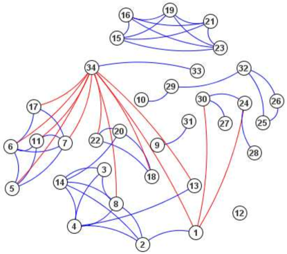
Figure 1: $\tilde{p}^{\{v,w\}}$ plot for Zachary’s karate club: blue: $\tilde{p}^{\{v,w\}}\geq 60\%$; red: $\tilde{p}^{\{v,w\}}\leq 1.8\%$

Figure 1 shows which pairs of nodes are particularly likely or unlikely to be in the same community for Zachary’s karate club data [79]. This is a social network of 34 members of a karate club at a university which split into two communities. Nodes 4 and 8 are most likely, with $\tilde{p}^{\{4,8\}}=98.8\%$, and nodes 1 and 34 least likely to be in the same community with $\tilde{p}^{\{1,34\}}=0.65\%$. Being adjacent does not guarantee a high value of $\tilde{p}^{\{v,w\}}$: the node pairs $\{1,32\}$ and $\{14,34\}$ each have $\tilde{p}^{\{v,w\}}=8.9\%$. Nor is it necessary for nodes to be adjacent to have a high value of $\tilde{p}^{\{v,w\}}$: among nodes 15, 16, 19, 21, and 23 $\tilde{p}^{\{v,w\}}=84.5\%$ for every pair, and $\tilde{p}^{\{8,14\}}=96.1\%$. Note that the node pairs $\{8,14\}$ and $\{1,34\}$ are each non-adjacent, and each has four common neighbors (i.e., $n_{2}=4$), but their values of $\tilde{p}^{\{v,w\}}$ differ by a factor of 150 because of the degrees of the nodes involved. Finally, although nodes 9 and 31 are in different ground-truth communities, $\tilde{p}^{\{9,31\}}=92.1\%$.

When numerical integration is not feasible, it is difficult to obtain good asymptotic estimates as $n\rightarrow\infty$, so we will resort to heuristics. The function $f$ has a global maximum which is increasingly sharp as $n\rightarrow\infty$. This occurs at

$$\delta_{p}\doteq\frac{n_{1}+2n_{2}}{2(n-2)},\quad\psi_{p}\doteq\frac{4n_{0}n_{2}-n_{1}^{2}}{4(n-2)^{2}}.$$ (3.26)

If $\psi_{p}\geq 0$, then this peak lies within $R^{+}$ when $\psi_{p}/(\psi_{p}+(1-\delta_{p})^{2})\leq\mu\leq\delta_{p}^{2}/(\psi_{p}+\delta_{p}^{2}).$ Assuming the expectation $\mathbb{E}_{m}[\cdot]$ has significant weight in this range, one can replace $f$ with a delta function at $(\delta_{p},\psi_{p})$ to estimate $\mathbb{E}[\Xi_{vw}|M_{vw}=1]$ (i.e., parameter estimation is an appropriate approximation to the full, Bayesian integration). To estimate $\mathbb{E}[\Xi_{vw}|M_{vw}=0]$ in this case, one could make the same argument, but with the maximum of $f(\delta,\psi^{-})$ constrained to $\psi^{-}\leq 0$. Conveniently, this constrained maximum occurs at $(\delta_{p},0)$. The analogous argument works when $\psi_{p}\leq 0$. Therefore, if the integrals in (3.24) and (3.25) contained nothing but $f(\delta,\psi)$ we could approximate them by $f(\delta_{p},\psi_{p})$ or $f(\delta_{p},0)$ as appropriate. Ignoring the expectation over $m$ as well, we could substitute these expressions into (3.7) to obtain the following approximation

$$\widetilde{\Lambda}_{vw}\approx\begin{cases}f(\delta_{p},\psi_{p})/f(\delta_{p},0)&\mathrm{if}\;\psi_{p}\geq 0,\;\text{and}\\ f(\delta_{p},0)/f(\delta_{p},\psi_{p})&\mathrm{if}\;\psi_{p}<0.\end{cases}$$ (3.27)

We may decompose $\Lambda$ as $\Lambda=\widetilde{\Lambda}\Lambda_{k}$, where $\Lambda_{1}$ encompasses all corrections to the crude approximation $\widetilde{\Lambda}$ when there is an edge between $v$ and $w$, and $\Lambda_{0}$ when there is no edge. For this, we need to specify the prior on $m$. Here, we let $\log m$ vary uniformly from $\log 2$ to $\log n$. It is convenient to treat $m$ (or, equivalently, $\mu$) as a continuum variable here to avoid the accidents of discreteness. With this prior, we may compute the value of $\mathbb{E}[M_{vw}]$ required in (3.6) as

$$\bar{\mu}=\mathbb{E}[M_{vw}]=\frac{1/2-1/n}{\log(n/2)}.$$ (3.28)

When $\psi_{p}$ differs greatly from 0, the $\widetilde{\Lambda}$ factor is very large or small and dominates the correction term $\Lambda_{k}$. Therefore we seek to approximate the correction factor only in the critical case $\psi_{p}=0$. Typically, real-world graphs are sparse, in which case the lack of an edge between $v$ and $w$ decreases their co-membership probability only slightly, but the presence of an edge greatly enhances it. Numerical experimentation confirms this intuition: the correction factor $\Lambda_{0}$ due to the absence of an edge is roughly constant, but the factor $\Lambda_{1}$ due to the presence of the edge $\{v,w\}$ increases rapidly as $\delta_{p}$ decreases until it hits a constant plateau (which varies with $n$):

$$\Lambda_{0} =\min(0.7197,0.46\,\delta_{p}^{-0.15}),\;\text{and}$$ (3.29)

$$\Lambda_{1} =\min(0.5605\,n+1.598,\delta_{p}^{-0.7}).$$ (3.30)

The four-digit coefficients in these formulas are obtained from an asymptotic analysis of exact results obtained in the $n_{1}=n_{2}=0$ case. These exact results involve combinations of generalized hypergeometric functions (i.e., ${}_{p}F_{q}(a;b;z)$), and are not particularly enlightening, although they can be used to obtain accurate coefficients, such as 0.56051044368284805729 rather than 0.5605 in (3.30).

Putting the above together into (3.6), we obtain the following approximation to $p^{\{v,w\}}$:

$$\hat{p}^{\{v,w\}}=\frac{\Lambda_{\kappa_{vw}}\widetilde{\Lambda}}{\Lambda_{\kappa_{vw}}\widetilde{\Lambda}+\bar{\mu}^{-1}-1}.$$ (3.31)

This formula could certainly be improved. It often yields results such as $\hat{p}^{\{v,w\}}=1-10^{-20}$: this figure might be accurate given the model assumptions, but such certainty could never be attained in the real world. To make it more accurate a more sophisticated model could be used, or the priors on $p_{I}$, $p_{O}$, and $m$ could be matched more closely to reality. Only limited improvement is possible, however, because in reality multiple, overlapping, fuzzily-defined community structures typically exist at various scales, and it is unclear what $p^{\{v,w\}}$ means in such a context. Certainly the integral approximations could be performed more rigorously and accurately. The broad outlines of the behavior of $p^{\{v,w\}}$ are captured in $\widetilde{\Lambda}$, $\Lambda_{0}$, and $\Lambda_{1}$, however. Finally, using only local evidence constitutes a rather radical pruning of the information in $G$. However, it is because of this pruning that the approximation (3.31) can be implemented so efficiently.

4 Community Detection: Results

Direct visualizations like Figure 1 are impractical for larger networks. It can be useful to use the blue edges in Figure 1 (those with $p^{\{v,w\}}$ above a certain threshold) in place of a graph’s edges in network algorithms (such as graph layout): this is discussed in Section 4.3. However, a more direct use of the co-membership matrix $p^{\{v,w\}}$ for network visualization is simply to plot the matrix itself with the values of $p^{\{v,w\}}\in[0,1]$ as intensities [61, 62]. An example of this is shown in Figure 2, using the approximation (3.31), for the Enron email communication network, which has 36,692 nodes and 367,662 edges [48]. The insets depict the hierarchical organization of community structure in networks [12, 44]: communities with various structures exist at all scales. Although the model $H(n,m,p_{I},p_{O})$ does not account for hierarchical structure, a benefit of integrating over the number of communities $m$ (rather than estimating it) is that this accounts for co-membership at different scales.

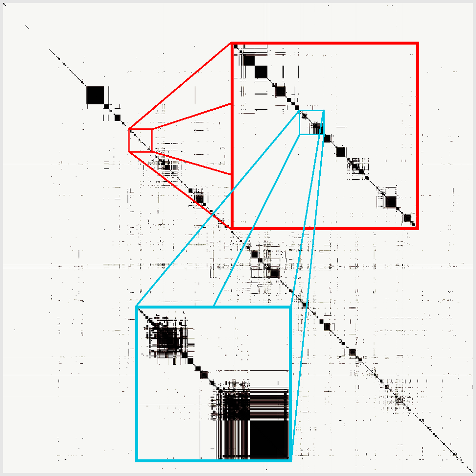
Figure 2: Visualization of $\hat{p}^{\{v,w\}}$ matrix for the Enron email network

4.1 Accuracy

One may rightly question whether the approximation $\hat{p}^{\{v,w\}}$ is accurate, given the modeling assumptions and approximations that it is based on. To address this, we observe that the values of $p^{\{v,w\}}$ may be used to define a certain family expected utility functions (parameterized by a threshold probability $\theta$: cf. (A.14) in Appendix A), and optimizing this expected utility yields a traditional community detection algorithm. Because a great many community detection algorithms have been developed, one can assess the quality of the approximation $\hat{p}^{\{v,w\}}\approx p^{\{v,w\}}$ by comparing the performance of the resulting community detection algorithm to those in the literature.

The most comprehensive comparison to date is based on the LFR benchmark graphs which have power-law distributions both on degree and on community size [43]. The conclusion is that all algorithms prior to 2008 were eclipsed by a set of three more recent algorithms: the Louvain algorithm [8], the Ronhovde–Nussinov (RN) algorithm [63], and Infomap [64]. Infomap performed somewhat better than RN, and both somewhat better than Louvain, but all three were much better than the previous generation. Figure 3 compares our algorithm to the Infomap, RN, and Louvain algorithms, and to the other algorithms tested in [43]. (This figure is a correction of Figure 3 from [27]. Also, the Simulated Annealing method which works so well in panel (b) is highlighted (purple with shorter dashes) in all panels for comparison.) Our method is labeled $U_{opt}$ because numerical optimization over all $\theta\in[0,1]$ has been used to set $\theta$ to the value that maximizes NMI. Both the 1000- and 5000-node cases are shown, for small communities (10 to 50 nodes) and large ones (20 to 100). The $x$-axis is the mixing parameter $\mu$—the fraction of a node’s neighbors outside its community (not the expected edge probability $\mu$ of (3.12))—and the $y$-axis is a particular version (cf. the appendix of [44]) of the Normalized Mutual Information (NMI) between the computed and the true partition. In all cases, our method $U_{opt}$ exhibits the performance characteristic of the three state-of-the-art methods cited by [43]. The $U_{opt}$ method has an unfair advantage in optimizing over all $\theta$: in a deployable algorithm one would need a method for setting $\theta$. On the other hand, the purpose of Figure 3 is simply to show that the $\hat{p}^{\{v,w\}}$ computation retains enough information about community structure to reconstruct high-quality hard-call solutions. From this perspective, it is surprising that it does so well, because $U_{opt}$ is based on (a) the simple utility function of Appendix A, (b) an approximation $\tilde{p}^{\{v,w\}}$ to $p^{\{v,w\}}$ based only on limited evidence, and (c) an approximation $\hat{p}^{\{v,w\}}$ to $\tilde{p}^{\{v,w\}}$ based on a heuristic evalution of the required integral.

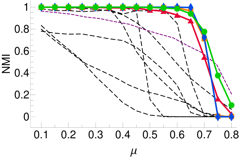
(a) 1000 nodes, small communities

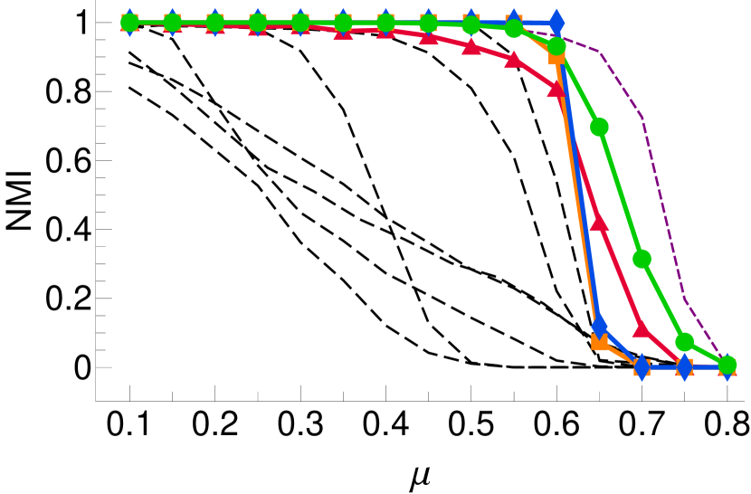
(b) 1000 nodes, large communities

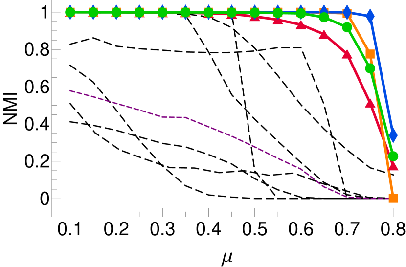
(c) 5000 nodes, small communities

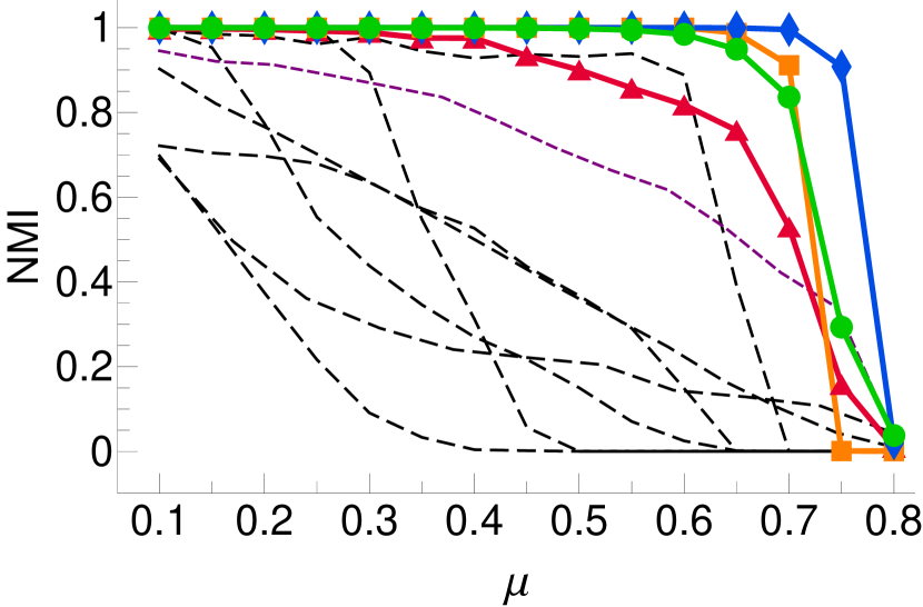
(d) 5000 nodes, large communities

Figure 3: Comparison of community detection algorithms:   ${\color[rgb]{0,0.8,0}\bullet}$: $U_{opt}$; ${\color[rgb]{0,0.3,0.9}\blacklozenge}$: Infomap; ${\color[rgb]{1,0.5,0}\scriptstyle\blacksquare\,}$: RN; ${\color[rgb]{0.9,0,0.2}\blacktriangle}$: Louvain; - - - : Other methods.

4.2 Efficiency

The algorithm for computing the $\hat{p}^{\{v,w\}}$ begins with pre-computing the value of $n_{2}$ for all pairs of nodes for which $n_{2}>0$, then creating a cache of $\hat{p}^{\{v,w\}}$ values for triples $(\kappa_{vw},n_{1},n_{2})$. For any node pair $\{v,w\}$, the value of $\hat{p}^{\{v,w\}}$ can be computed by first looking up its value of $n_{2}$, computing $n_{0}$ and $n_{1}$ from $n$ and the degrees of $v$ and $w$, then looking up the $\hat{p}^{\{v,w\}}$ value for its triple $(\kappa_{vw},n_{1},n_{2})$. Occasionally the value for this triple must be computed from (3.31) and cached, but the number of such distinct triples is relatively small in practice. An optional additional step one can perform is to loop over all node pairs with non-zero $n_{2}$ in order to both fill in the value of $\hat{p}^{\{v,w\}}$ for each triple $(\kappa_{vw},n_{1},n_{2})$, and count the number of times each triple occurs. (Because only the $\{v,w\}$ pairs with $n_{2}>0$ are looped over, some additional bookkeeping is needed to fill in and provide a count for the $(\kappa_{vw},n_{1},0)$ triples without actually iterating over all $O(n^{2})$ node pairs.) These values and counts are useful for the statistical analysis of the $\hat{p}^{\{v,w\}}$ distribution.

We tested the algorithm on five different Facebook networks (gathered from various universities) [74], and networks generated from Slashdot [49], Amazon [47], LiveJournal [49], and connections between .edu domains (Wb-edu) [19]. Table 1 shows various relevant network statistics. The sum of the values $n_{2}$ for each node pair is the number of calculations needed to compute the $n_{2}$ data structure, whereas the number of values of $n_{2}>0$ reflects its size. The next column is the number of distinct $(\kappa_{vw},n_{1},n_{2})$ triples—this is the number of distinct $\hat{p}^{\{v,w\}}$ values that must be computed, and the final one is the number of communities that a randomly chosen instance of the algorithm Infomap [64] found for the dataset. For the last two rows the $n_{2}$ data structure was too large to hold in memory, and the second step of counting the triples was not performed, nor could Infomap be run successfully on our desktop.

$${\small\begin{array}[]{|l|r|r|r|r|r|r|}\hline\cr\vrule\lx@intercol\hfil\text{Dataset}\hfil\lx@intercol\vrule\lx@intercol&\lx@intercol\hfil\;\text{Nodes}\hfil\lx@intercol\vrule\lx@intercol&\lx@intercol\hfil\;\text{Edges}\hfil\lx@intercol\vrule\lx@intercol&\lx@intercol\hfil\;\sum n_{2}\hfil\lx@intercol\vrule\lx@intercol&\lx@intercol\hfil\;\#(n_{2}>0)\hfil\lx@intercol\vrule\lx@intercol&\lx@intercol\hfil\;\;\text{Triples}\hfil\lx@intercol\vrule\lx@intercol&\lx@intercol\hfil\;\text{Groups}\hfil\lx@intercol\vrule\lx@intercol\\ \hline\cr\text{Caltech}&769&16,\!656&1,\!231,\!412&186,\!722&14,\!120&19\\ \hline\cr\text{Princeton}&6,\!596&293,\!320&46,\!139,\!701&8,\!776,\!074&83,\!004&51\\ \hline\cr\text{Georgetown}&9,\!414&425,\!638&67,\!751,\!053&15,\!616,\!610&113,\!722&90\\ \hline\cr\text{Oklahoma}&17,\!425&892,\!528&194,\!235,\!901&47,\!202,\!925&239,\!162&233\\ \hline\cr\text{UNC}&18,\!163&766,\!800&140,\!796,\!299&47,\!576,\!619&191,\!482&167\\ \hline\cr\text{Slashdot}&82,\!168&504,\!230&74,\!983,\!589&49,\!450,\!449&104,\!330&5,\!209\\ \hline\cr\text{Amazon}&262,\!111&899,\!792&9,\!120,\!350&6,\!434,\!638&7,\!178&\;12,\!851\\ \hline\cr\text{LiveJournal}&4,\!847,\!571&42,\!851,\!237&7,\!269,\!503,\!753&4,\!193,\!393,\!006&&\\ \hline\cr\text{Wb-edu}&\;9,\!450,\!404&\;46,\!236,\!105&\;12,\!203,\!737,\!639&\;4,\!232,\!928,\!806&&\\ \hline\cr\end{array}}$$

Table 1: Network datasets

Table 2 contains timing results based on a Dell desktop with 8GB of RAM, and eight 2.5GHz processors. The first column is the number of seconds it took the version of Infomap described in [64] to run. This code is in C++, runs single-threaded, includes a small amount of overhead for reading the network, and uses the Infomap default setting of picking the best result from ten individual Infomap trial partitions. The next four columns compare methods of using our Java code to compute $n_{2}$. The first two are single-threaded, and the other two use all eight cores. The columns labeled $n_{2}\rightarrow\emptyset$ are the timing for the computation only: results are nulled out immediately after computing them. These columns are included for two reasons. First, they show that the computation itself displays good parallelization: the speedup is generally higher than 6.5 for eight processors. Second, the computation itself for the two larger datasets is quite fast (just under three minutes on eight cores), but the algorithm is currently designed only to maintain all results in RAM, and these datasets are too large for this. The last two columns are the timing results for explicitly filling in the $\hat{p}^{\{v,w\}}$ information ahead of time and providing the counts required for statistical analysis.

As Infomap is one of the fastest community detection algorithms available, these results are quite impressive. Comparing the first two columns of timing data, we find the speed-up ranges up to 107 and 862 times as fast as Infomap for the two largest networks on which we ran Infomap, respectively. The relative performance falls off rapidly for denser networks, but even in these cases or method performed roughly 10 times as fast as Infomap (i.e., as fast as an individual Infomap run). Computing the counts for $\hat{p}^{\{v,w\}}$ statistics increases the run time, but only by a constant factor (of 2 to 3). It must be emphasized that the timing results are for producing a very different kind of output than Infomap does. However, the usual method for estimating $p^{\{v,w\}}$ [62] is many times slower than producing partitions, rather than many times faster.

$${\small\begin{array}[]{|l|D{.}{.}{1}|D{.}{.}{2}|D{.}{.}{2}|D{.}{.}{2}|D{.}{.}{2}|D{.}{.}{2}|D{.}{.}{2}|}\hline\cr\vrule\lx@intercol\hfil\hbox{\multirowsetup Dataset}\hfil\lx@intercol\vrule\lx@intercol&\lx@intercol\hfil\;\text{Infomap}\hfil\lx@intercol\vrule\lx@intercol&\lx@intercol\hfil n_{2}\hfil\lx@intercol\vrule\lx@intercol&\lx@intercol\hfil\;n_{2}\rightarrow\emptyset\hfil\lx@intercol\vrule\lx@intercol&\lx@intercol\hfil n_{2}\hfil\lx@intercol\vrule\lx@intercol&\lx@intercol\hfil\;n_{2}\rightarrow\emptyset\hfil\lx@intercol\vrule\lx@intercol&\lx@intercol\hfil\;\text{Count}\hfil\lx@intercol\vrule\lx@intercol&\lx@intercol\hfil\;\text{Count}\hfil\lx@intercol\vrule\lx@intercol\\ \vrule\lx@intercol\hfil\hfil\lx@intercol\vrule\lx@intercol&\lx@intercol\hfil\;10\;\text{trials}\hfil\lx@intercol\vrule\lx@intercol&\lx@intercol\hfil\;1\;\text{proc}\hfil\lx@intercol\vrule\lx@intercol&\lx@intercol\hfil\;1\;\text{proc}\hfil\lx@intercol\vrule\lx@intercol&\lx@intercol\hfil\;8\;\text{proc}\hfil\lx@intercol\vrule\lx@intercol&\lx@intercol\hfil\;8\;\text{proc}\hfil\lx@intercol\vrule\lx@intercol&\lx@intercol\hfil\;1\;\text{proc}\hfil\lx@intercol\vrule\lx@intercol&\lx@intercol\hfil\;8\;\text{proc}\hfil\lx@intercol\vrule\lx@intercol\\ \hline\cr\text{Caltech}&.0$&0.11$&0.09$&0.02$&0.02$&0.09$&0.03$\\ \hline\cr\text{Princeton}&45.4$&4.5$&3.9$&0.67$&0.55$&3.9$&0.70$\\ \hline\cr\text{Georgetown}&77.5$&7.2$&6.4$&1.2$&0.93$&7.0$&1.2$\\ \hline\cr\text{Oklahoma}&310.8$&3.5$&19.4$&4.2$&.8$&33.7$&4.6$\\ \hline\cr\text{UNC}&446.6$&19.2$&16.3$&3.6$&.5$&2.9$&4.0$\\ \hline\cr\text{Slashdot}&553.4$&14.5$&12.6$&3.0$&1.9$&1.8$&3.6$\\ \hline\cr\text{Amazon}&2075.8$&.4$&.2$&0.59$&0.44$&3.2$&0.69$\\ \hline\cr\text{LiveJournal}&$&$&1246.2$&$&172.9$&$&$\\ \hline\cr\text{Wb-edu}&$&$&1243.0$&$&174.6$&$&$\\ \hline\cr\end{array}}$$

Table 2: Timing results (in seconds)

4.3 Uses

Visualizing the $\hat{p}^{\{v,w\}}$ matrix provides insight into the hierarchical community structure of a network [62]. To do so requires an appropriate ordering on the nodes: one that places nodes nearby when they are in the same small community, and small communities nearby when they are in the same larger community. Therefore, it is useful to have a dendrogram of hierarchical community clustering. There are standard routines for producing such dendrograms, provided one has a distance metric between points [36]. The community non-co-membership probabilities $p^{\{v\}\{w\}}=1-p^{\{v,w\}}$ may be used for this purpose. They satisfy the triangle inequality $p^{\{v\}\{w\}}\leq p^{\{v\}\{x\}}+p^{\{w\}\{x\}}$ (although distinct nodes have distance 0 between them if they are known to be in the same community). The approximation (3.31) does not obey this triangle inequality, however, and [26] indicates that this can cause problems in certain contexts. An approximation of $p^{\{v,w\}}$ which does obey it is a topic for future research. In the meantime, we will rely on this version, which tends to obey it for most node triples.

To order the nodes of a graph we use this (approximate) distance metric $p^{\{v\}\{w\}}$ with a hierarchical clustering scheme that defines cluster distance as the average distance between nodes. The output of this is a binary tree (ties having been broken arbitrarily), so the order of the clusters at each branch point must still be determined. This is done by starting at the root of the tree and testing which ordering at each branch point yields a smaller average distance to its neighboring clusters on the right and left. Figure 4 shows the resulting dendrogram for the Princeton Facebook network (cf. Table 1), and the corresponding $\hat{p}^{\{v,w\}}$ matrix. (This method was used to generate the ordering in Figure 2 as well.)

(a) Dendrogram for node ordering

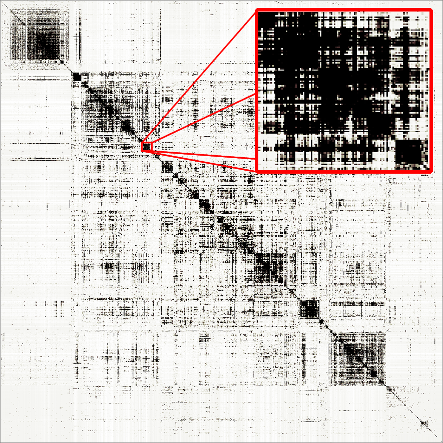
(b) $\hat{p}^{\{v,w\}}$ matrix

Figure 4: Visualization of community structure for Princeton Facebook network

Visualizations like Figure 4 are useful for network analysis. We have combined them other visualizations in the code IGNITE (Inter-Group Network Inference and Tracking Engine). Figure 5 uses IGNITE to the Georgetown Facebook network (cf. Table 1). The dendrogram on which the ordering for the $\hat{p}^{\{v,w\}}$ matrix is based is shown in the upper left panel. Two levels in this dendrogram have been selected: the lower level is used to coarse-grain the network by merging communities of nodes together into meta-nodes; the upper level is used to determine which sets of meta-nodes to consider communities. The selection of these levels is reflected in the $\hat{p}^{\{v,w\}}$ matrix panel below. The meta-nodes are indicated by translucent green squares, and communities of nodes are outlined in different colors (corresponding to similar outlines in the dendrogram). The meta-nodes and communities are then displayed in panels on the right: the upper panel corresponding to a coarse-grained version of the original network; the lower, to a variant where the edges have been replaced with averaged $\hat{p}^{\{v,w\}}$ values between meta-nodes. The sizes of the meta-nodes indicates how many true nodes they contain. In the lower right panel, blue lines indicate average $\hat{p}^{\{v,w\}}$ above a certain threshold, and red below another (much lower) threshold, as in Figure 1.

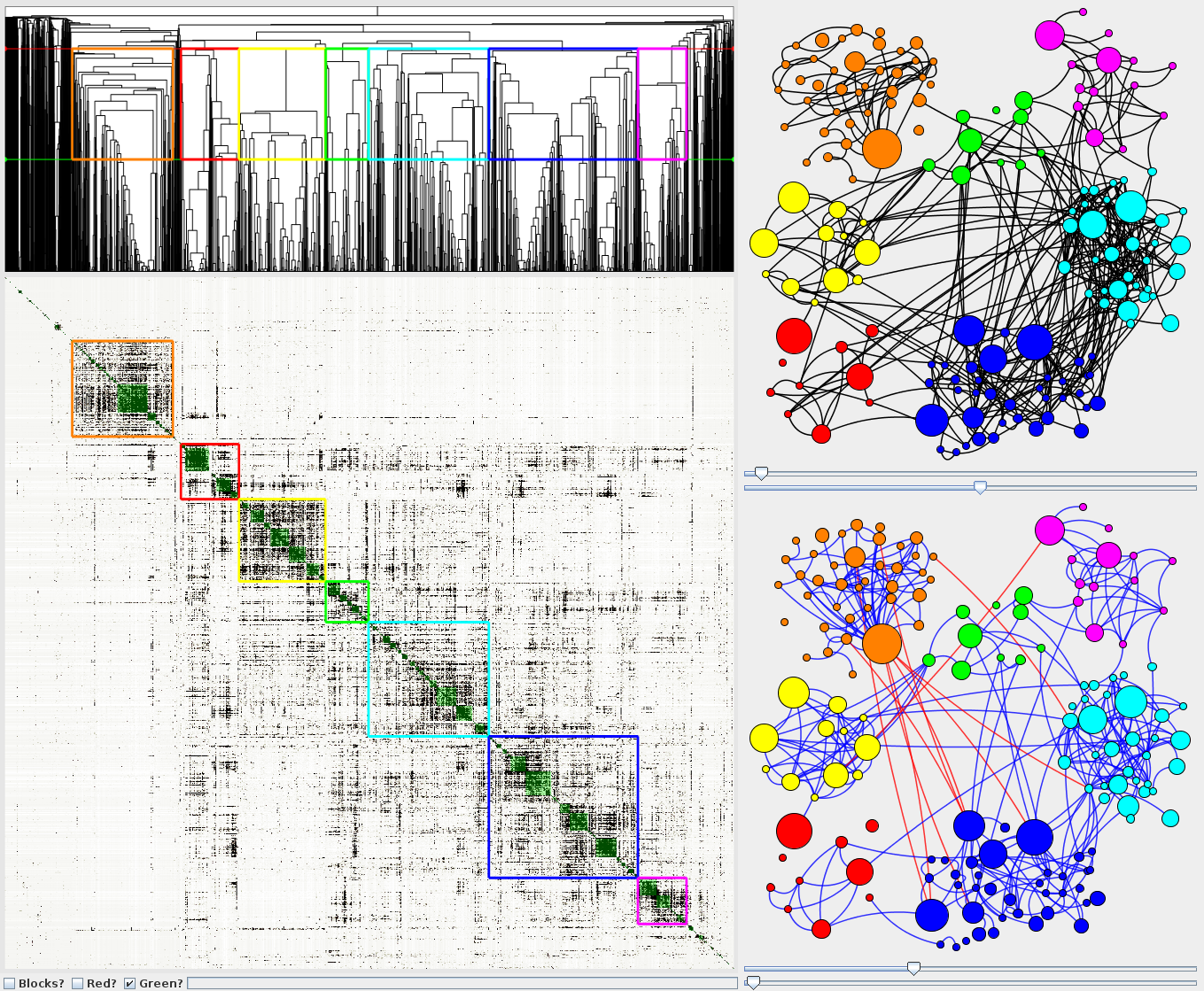
Figure 5: Screen shot of IGNITE network probability visualization tool for Georgetown Facebook network

5 Community Tracking: Exact Equations

The study of dynamic networks is much less developed than its static counterpart. There is substantial work on processes evolving on networks. For example, see [18] for a discussion of the complex dynamical systems which arise in economics and traffic engineering, along with mathematically rigorous results about their equilibria. Diffusion equations on networks have particularly elegant properties. They are governed by the Laplacian matrix of a graph, the discrete analog of continuum Laplacian operator, and are therefore an important topic in spectral graph theory [54]. These may be generalized to reaction–diffusion equations and used to model the spread of disease [13], but the more common model in network epidemiology is the SIR model [42]. Such models have been extended to model the spread of rumors [3], obesity [11], and innovations [75].

The term “dynamic networks” implies that the networks themselves are evolving in time, however. Stokman and Doreian edited several influential special editions of the Journal of Mathematical Sociology on network evolution, the first of which was in 1996 and published in book form as [21]. This work illustrated how macroscopic behavior of network evolution arises from local governing laws. Snijders emphasizes [68] the benefits of casting the dynamic network problem in the continuous-time, Markov process framework first proposed by Leenders [46]. In particular, there is a small body of literature on communities evolving in dynamic networks. Much of this work is summarized in 3 1/2 pages of Fortunato’s 100-page review of group finding [28]. The field begins with the 2004 work of Hopcroft et al. [35], which studied the persistence of robust communities in the NEC CiteSeer database. The most prominent publication is the 2007 work of Palla et al. [59], which analyzed the evolution of overlapping groups in cell phone and co-authorship data and presented a method for tracking communities based on the clique percolation method used in CFinder [60]. The various researchers in the community have come to agree on the key fundamental events of community evolution: birth/death, expansion/contraction, and merging/splitting [31]. Berger-Wolf and colleagues propose an optimality criterion for assigning time-evolving community structure to a sequence of network snapshots, prove that it is NP-hard to find the optimal structure, and develop various approximation techniques [73, 72, 71].

Most of the work on community tracking considers discrete network snapshots and attempts to match up the community structure at different time steps. From the perspective of the data fusion community, such an approach to tracking may seem ad hoc: one could argue that (a) the “matching up” criteria are necessarily heuristic, and (b) one gets only a single best solution with no indication of the uncertainty. In contrast, the tracking work in data fusion is based on formal evolution and measurement models for the full probability distribution over some state space, followed by principled approximations [39]. A sensible response to this critique, however, is that the state space in the community tracking problem is so much larger that data-fusion-style tracking techniques do not apply. The truth is perhaps somewhere in between: it is, in fact, possible to derive a formal Bayesian filter for the community tracking problem and to produce tractable approximations to it. Indeed, this is the topic of the remainder of this paper. On the other hand, the filter derived is more a proof of concept than an algorithm ready to supplant the more informal methods. It may be that the formal approach we present here can be developed into a true, practical “Kalman filter for networks.” On the other hand, it may be that concerns about uncertainty management can be addressed without appeal to a formal model. For example, Rosvall and Bergstrom have devised a re-sampling technique to estimate the degree to which the data support the various assignments of nodes to time-evolving communities [65]. Similarly, the work of Fenn et al. tracks the evolution of groups by gathering evidence that each node belongs to one of a number of known groups [23], thus providing output similar to one version of the method outlined below.

We model community and graph evolution as a continuous-time Markov process [16], $\{(\Phi_{t},\mathrm{K}_{t}):t\geq 0\}$, the continuous-time analog of a Markov chain. The continuous-time approach is more general (in that it can always be sampled at discrete times to produce a Markov chain) and is simpler to work with due to the sparsity of the matrices involved. We will not explicitly indicate any dependence on structural parameters $\vec{\mu}$, because we will not integrate these out as was done in the static case. In this section we will use $\mathrm{K}_{[0,t]}\doteq\{\mathrm{K}_{t^{\prime}}:0\leq t^{\prime}\leq t\}$ to denote the time-history of the network process up through time $t$, and $\mathrm{K}_{[0,t)}\doteq\{\mathrm{K}_{t^{\prime}}:0\leq t^{\prime}<t\}$ for the history not including the current time $t$ (with similar definitions for $\Phi_{[0,t]}$ and $\Phi_{[0,t)}$). The purpose of this section is to derive a Bayesian filter $\mathrm{Pr}(\Phi_{t}|\mathrm{K}_{[0,t]})$: i.e., assuming some initial distribution $\mathrm{Pr}(\Phi_{0})$ is given, Section 5.1 derives the expressions for evolving the distribution of the community structure to time $t$, given all network evidence up through time $t$. In the community detection case, the next step was to approximate marginals of the full distribution using limited graph evidence. In the tracking case, however, it is possible to obtain exact formulas for the marginals: this is done in Section 5.2. These formulas, though exact, are not closed, however: the approximations required to close them are discussed in Section 6.

5.1 Evolution of the full distribution

A dynamic stochastic blockmodel $\mathcal{H}(n,A,\mathbf{B})$ may be defined analogously to the static version $H(n,\mathbf{p},\mathbf{Q})$ introduced in Section 2.1. Whereas $H(n,\mathbf{p},\mathbf{Q})$ defines a pair of random variables $\Phi$ and $\mathrm{K}$, $\mathcal{H}(n,A,\mathbf{B})$ defines a pair of stochastic processes $\{\Phi_{t}:t\geq 0\}$ and $\{\mathrm{K}_{t}:t\geq 0\}$. The joint process $\{(\Phi_{t},\mathrm{K}_{t}):t\geq 0\}$ will be modeled as a continuous-time Markov process. The parameter $A$ is an $m\times m$ matrix, and $\mathbf{B}$ is a collection of $r\times r$ matrices $B_{ij}$ for $1\leq i\leq j\leq m$ (and for convenience we define $B_{ji}=B_{ij}$ for $j>i$). Just as $\mathbf{p}$ and the $\mathbf{q}_{ij}$ were required to be stochastic vectors (i.e., vectors with non-negative entries that sum to one) in Section 2.1, so the matrices $A$ and $B_{ij}$ are required to be transition rate matrices: i.e., they must have non-negative off-diagonal entries, and their columns must sum to zero. The entry $a_{ij}$ of $A$ defines the transition rate of a node in group $j$ switching to group $i$: i.e., the probability of a node in group $j$ being in group $i$ after an infinitesimal time $\Delta t$ is $\delta_{ij}+a_{ij}\,\Delta t+O((\Delta t)^{2})$. Similarly, the entry $b_{ij,kl}$ of $B_{ij}$ defines the rate that an edge connecting nodes in groups $i$ and $j$ transitions from edge type $l$ to type $k$.

We may define a dynamic planted partition model $\mathcal{H}(n,m,a,\lambda_{I},\mu_{I},\lambda_{O},\mu_{O})$ as a special case of $\mathcal{H}(n,A,\mathbf{B})$. As in Section 2.2, this cases is obtained by requiring that $A$ and $\mathbf{B}$ be invariant under permutations of $[m]$ and using only $r=2$ edge types (“off” ($k=0$) and “on” ($k=1$)). In this case, the transition rate matrix $A$ reduces to a single rate $a$ at which nodes jump between communities, while the collection $\mathbf{B}$ of transition rate matrices reduces to four rate parameters: $\lambda_{I}$, the rate at which edges turn on for pairs of nodes in the same community; $\mu_{I}$, the rate at which edges turn off for pairs of nodes in the same community; and $\lambda_{O}$ and $\mu_{O}$, the corresponding rates for pairs of nodes in different communities. Figure 6 depicts and instance of this model with $n=12$ nodes and $m=3$ communities with rate parameters $a=0.5$, $\lambda_{I}=16$, $\mu_{I}=4$, $\lambda_{O}=2$, and $\mu_{O}=18$ for $t=0$ to 5.

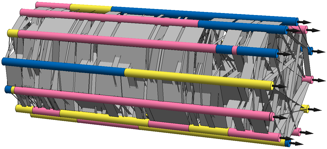
Figure 6: An instance of $\mathcal{H}(12,3,0.5,16,4,2,18)$

If two independent random variables $X$ and $Y$ have respective probabilities $x_{i}$ and $y_{j}$ for their various outcomes $i$ and $j$, then the joint random variable $Z=(X,Y)$ has outcomes indexed by $(i,j)$ with probabilities $z_{(i,j)}=x_{i}y_{j}$. The analog of this for Markov processes is expressed by the Kronecker sum [58]. I.e., Suppose two independent Markov processes $\{X(t):t\geq 0\}$ and $\{Y(t):t\geq 0\}$ have respective probabilities $x_{i}(t)$ and $y_{j}(t)$ for their various outcomes $i$ and $j$ at time $t$, and that these probabilities are governed by $\dot{\mathbf{x}}=A\mathbf{x}$ and $\dot{\mathbf{y}}=B\mathbf{y}$, respectively (where $\mathbf{x}(t)$ collects all the $x_{i}(t)$, and $\mathbf{y}(t)$, the $y_{j}(t)$). Then the joint Markov process $\{Z(t):t\geq 0\}$, where $Z(t)=(X(t),Y(t))$, has outcomes indexed by $(i,j)$ with probabilities $z_{(i,j)}$ that are governed by $\dot{\mathbf{z}}=(A\oplus B)\mathbf{z}$ (where $\mathbf{z}(t)$ collects all the $z_{(i,j)}$). The Kronecker sum $A\oplus B$ is defined by

$$(A\oplus B)_{(i,j),(i^{\prime},j^{\prime})}\doteq a_{ii^{\prime}}\delta_{jj^{\prime}}+\delta_{ii^{\prime}}b_{jj^{\prime}}.$$ (5.1)

The interpretation of this is that in an infinitesimal time the Markov process $X_{t}$ may transition from $i$ to another state $i^{\prime}$, or $Y_{t}$ may transition from $j$ to $j^{\prime}$, but for both to change simultaneously is infinitely less likely than for only one to change.

The derivation of the Bayesian filter for $\mathrm{Pr}(\Phi_{t}|\mathrm{K}_{[0,t]})$ follows the same six steps as the static derivation in Section 2.1. Indeed, the purpose of including the six-step derivation in Section 2.1 was to make the following derivation easier to follow by analogy.

Step 1. Let $\mathbf{p}^{v}(t)\in\mathbb{R}^{m}$ denote the vector of probabilities $p^{v}_{i}(t)$ that a single node $v$ is in community $i$ at time $t$: i.e., $p^{v}_{i}(t)\doteq\mathrm{Pr}(\Phi_{t}(v)=i)$. These probabilities are governed by the transition rate matrix $A$. Therefore

$$\frac{d\mathbf{p}^{v}}{dt}=A\mathbf{p}^{v},\quad\text{which has the solution}\;\;\mathbf{p}^{v}(t^{\prime})=e^{A(t^{\prime}-t)\mathbf{p}^{v}(t)}.$$ (5.2)

Step 2. Let $\mathcal{P}\in\mathbb{R}^{m^{n}}$ denote the vector of probabilities $\mathcal{P}_{\phi}(t)$ that the communities of all $n$ nodes are specified by the assignment $\phi$ at time $t$: i.e., $\mathcal{P}_{\phi}(t)\doteq\mathrm{Pr}(\Phi_{t}=\phi)$. The transition rate matrix for this joint process on all nodes is the Kronecker sum of the (identical) transition rate matrices for each node:

$$\frac{d\mathcal{P}}{dt}=\mathcal{A}\mathcal{P},\quad\text{where}\;\;\mathcal{A}=\bigoplus_{v=1}^{n}A.$$ (5.3)

The components $\mathcal{A}_{\phi^{\prime}\phi}$ of $\mathcal{A}$ may be expressed as

$$\mathcal{A}_{\phi^{\prime}\phi}=\begin{cases}\displaystyle\sum_{v=1}^{n}a_{\phi(v)\phi(v)},\quad&\text{if}\;\phi^{\prime}=\phi,\\ a_{\phi^{\prime}(v^{*})\phi(v^{*})},&\text{if}\;\phi^{\prime}(v)=\phi(v)\;\text{for all}\;v\neq v^{*},\\ 0,&\text{otherwise}.\end{cases}$$ (5.4)

Step 3. Let $\mathbf{q}^{e}(t)\in\mathbb{R}^{N}$ (where $N=n(n-1)/2$) denote the vector of probabilities $q^{e}_{k}(t)$ that a single edge $e$ has type $k$ at time $t$ given the current communities of its endpoints: i.e., $q^{e}_{k}(t)\doteq\mathrm{Pr}(\mathrm{K}_{t}(e)=k|\Phi_{t}(v),\Phi_{t}(w))$. These probabilities are governed by the transition rate matrix $B_{ij}$, where $i=\phi_{t}(v)$ and $j=\phi_{t}(w)$ are the current communities of $v$ and $w$:

$$\frac{d\mathbf{q}^{e}}{dt}=B_{\phi_{t}(v)\phi_{t}(w)}\mathbf{q}^{e}.$$ (5.5)

The matrix $B_{\phi_{t}(v)\phi_{t}(w)}$ is piecewise constant in time, so the solution to (5.5) is a (continuous) piecewise exponential function.

Step 4. Let $\mathcal{Q}\in\mathbb{R}^{r^{N}}$ denote the vector of probabilities $\mathcal{Q}_{\kappa}(t)$ that the graph is $\kappa$ at time $t$ given the current communities of all nodes: i.e., $\mathcal{Q}_{\kappa}(t)\doteq\mathrm{Pr}(\mathrm{K}_{t}=\kappa|\Phi_{t})$. The transition rate matrix for this joint process on all edges is the Kronecker sum of the transition rate matrices for each edge:

$$\frac{d\mathcal{Q}}{dt}=\mathcal{B}_{\phi_{t}}\mathcal{Q},\quad\text{where}\;\;\mathcal{B}_{\phi}=\bigoplus_{e\in[n]^{\{2\}}}B_{\phi(e_{1})\phi(e_{2})}.$$ (5.6)

The components $\mathcal{B}_{\phi,\kappa^{\prime}\kappa}$ of $\mathcal{B}_{\phi}$ may be expressed as

$$\mathcal{B}_{\phi,\kappa^{\prime}\kappa}=\begin{cases}\displaystyle\sum_{e\in[n]^{\{2\}}}b_{\phi(e_{1})\phi(e_{2}),\kappa(e)\kappa(e)},\quad&\text{if}\;\kappa^{\prime}=\kappa,\\ b_{\phi(e_{1}^{*})\phi(e_{2}^{*}),\kappa^{\prime}(e^{*})\kappa(e^{*})},&\text{if}\;\kappa^{\prime}(e)=\kappa(e)\;\text{for all}\;e\neq e^{*},\\ 0,&\text{otherwise}.\end{cases}$$ (5.7)

Step 5. Let $\mathcal{R}\in\mathbb{R}^{m^{n}r^{N}}$ denote the vector of probabilities $\mathcal{R}_{(\phi,\kappa)}$ that the community assignment is $\phi$ and the graph is $\kappa$ at time $t$: i.e., $\mathcal{R}_{(\phi,\kappa)}(t)\doteq\mathrm{Pr}(\Phi_{t}=\phi,\mathrm{K}_{t}=\kappa)$. The transition rate matrix for this process is not quite a Kronecker sum due to the dependence of $\mathcal{B}_{\phi}$ on $\phi$—it loses the various nice properties that Kronecker sums have, but the formula is quite similar:

$$\frac{d\mathcal{R}}{dt}=\mathcal{C}\mathcal{R},\quad\text{where}\;\;\mathcal{C}_{(\phi^{\prime},\kappa^{\prime})(\phi,\kappa)}=\mathcal{A}_{\phi^{\prime}\phi}\delta_{\kappa^{\prime}\kappa}+\delta_{\phi^{\prime}\phi}\mathcal{B}_{\phi,\kappa^{\prime}\kappa}.$$ (5.8)

A Bayesian filter has a prediction step (which applies while the graph data remains constant) and an update step (which applies when the graph data changes). Therefore, we need to decompose (5.8) into a component which is zero while the graph is constant and a component which is zero when the graph changes. The required decomposition uses slightly modified matrices $\mathcal{A}^{\prime}_{\kappa}$ and $\mathcal{B}^{\prime}_{\phi}$:

$$\mathcal{C}_{(\phi^{\prime},\kappa^{\prime})(\phi,\kappa)} =\mathcal{A}^{\prime}_{\kappa,\phi^{\prime}\phi}\delta_{\kappa^{\prime}\kappa}+\delta_{\phi^{\prime}\phi}\mathcal{B}^{\prime}_{\phi,\kappa^{\prime}\kappa},\quad\text{where}$$ (5.9)

$$\mathcal{A}^{\prime}_{\kappa,\phi^{\prime}\phi} =\mathcal{A}_{\phi^{\prime}\phi}+\delta_{\phi^{\prime}\phi}\mathcal{B}_{\phi,\kappa\kappa},\quad\text{and}\quad\mathcal{B}^{\prime}_{\phi,\kappa^{\prime}\kappa}=\mathcal{B}_{\phi,\kappa^{\prime}\kappa}-\delta_{\kappa^{\prime}\kappa}\mathcal{B}_{\phi,\kappa\kappa}.$$ (5.10)

The components $\mathcal{A}^{\prime}_{\kappa,\phi^{\prime}\phi}$ of $\mathcal{A}^{\prime}_{\kappa}$ may be expressed as

$$\mathcal{A}^{\prime}_{\kappa,\phi^{\prime}\phi}=\begin{cases}\displaystyle\sum_{v=1}^{n}a_{\phi(v)\phi(v)}+\!\!\sum_{e\in[n]^{\{2\}}}b_{\phi(e_{1})\phi(e_{2}),\kappa(e)\kappa(e)},\quad&\text{if}\;\phi^{\prime}=\phi,\\ a_{\phi^{\prime}(v^{*})\phi(v^{*})},&\text{if}\;\phi^{\prime}(v)=\phi(v)\;\text{for all}\;v\neq v^{*},\\ 0,&\text{otherwise}.\end{cases}$$ (5.11)

The components $\mathcal{B}^{\prime}_{\phi,\kappa^{\prime}\kappa}$ of $\mathcal{B}^{\prime}_{\phi}$ may be expressed as

$$\mathcal{B}^{\prime}_{\phi,\kappa^{\prime}\kappa}=\begin{cases}\displaystyle b_{\phi(e_{1}^{*})\phi(e_{2}^{*}),\kappa^{\prime}(e^{*})\kappa(e^{*})},&\text{if}\;\kappa^{\prime}(e)=\kappa(e)\;\text{for all}\;e\neq e^{*},\\ 0,&\text{otherwise}.\end{cases}$$ (5.12)

Step 6. The prediction and update steps of the Bayesian filter are now determined by the matrices $\mathcal{A}^{\prime}$ and $\mathcal{B}^{\prime}$. For the prediction step, suppose that the graph data through time $t_{0}$ is $\kappa_{[0,t_{0}]}$ and let $\kappa=\kappa_{t_{0}}$ be a concise notation for the graph at time $t_{0}$. From a previous step of the filter (or from an initialization) we are given the distribution on the community assignments $\mathrm{Pr}(\Phi_{t_{0}}|\mathrm{K}_{[0,t_{0}]}=\kappa_{[0,t_{0}]})$. Starting with this distribution on $\phi$ at time $t_{0}$, let $\mathcal{R}_{\kappa}(t)\in\mathbb{R}^{m^{n}}$ (for all $t\geq t_{0}$) be a vector whose $\phi$ component is the probability that (a) the graph remains $\kappa$ during the time interval $[t_{0},t)$, and (b) the community assignment is $\phi$ at time $t$. The initial value of $\mathcal{R}_{\kappa}$ is then $\mathcal{R}_{\kappa}(t_{0})=\mathrm{Pr}(\Phi_{t_{0}}|\mathrm{K}_{[0,t_{0}]}=\kappa_{[0,t_{0}]})$. Its evolution law is given by

$$\frac{d\mathcal{R}_{\kappa}}{dt}=\mathcal{A}^{\prime}_{\kappa}\mathcal{R}_{\kappa}.$$ (5.13)

Note that $\mathcal{A}^{\prime}_{\kappa}$ is not a transition rate matrix: it allows probability to leak out of the vector $\mathcal{R}_{\kappa}(t)$ so that its sum does not remain 1, but rather equals the probability $\mathrm{Pr}(\mathrm{K}_{[t_{0},t)}=\kappa|\mathrm{K}_{[0,t_{0}]}=\kappa_{[0,t_{0}]})$. Normalizing $\mathcal{R}_{\kappa}(t)$, however, gives us the probability distribution of $\phi$ given that the graph has remained $\kappa$ during the time interval $[t_{0},t)$:

$$\mathrm{Pr}\big{(}\Phi_{t}=\phi|\mathrm{K}_{[0,t)}=\kappa_{[0,t)}\big{)}\propto\big{(}\mathcal{R}_{\kappa}(t)\big{)}_{\phi}.$$ (5.14)

This, then, is the prediction step of the Bayesian filter. The update step is obtained from $\mathcal{B}^{\prime}$: given that the community assignment is $\phi$, the probability of a single edge $e=\{v,w\}$ transitioning from type $k=\kappa_{t^{-}}(e)$ to type $k^{\prime}=\kappa_{t}(e)$ in some infinitesimal time period $\Delta t$ is given by (5.12) as $b_{\phi(v)\phi(w),k^{\prime}k}\Delta t$. The conditional probabilities of the posterior distribution on $\phi$ given this single edge transition are proportional to this. Therefore

$$\mathrm{Pr}\big{(}\Phi_{t}=\phi|\mathrm{K}_{[0,t]}=\kappa_{[0,t]}\big{)}\propto b_{\phi(v)\phi(w),k^{\prime}k}\mathrm{Pr}\big{(}\Phi_{t^{-}}=\phi|\mathrm{K}_{[0,t)}=\kappa_{[0,t)}\big{)}.$$ (5.15)

This equation holds only for a single edge transitioning. When multiple edges transition at exactly the same time, the correct update procedure would be to average, over all possible orderings of the edge transitions, the result of applying (5.15) successively to each transition.

Figure 7 shows the exact evolution for the very simple, dynamic planted partition case $\mathcal{H}(3,2,1,3,1,1,3)$. Here there are $n=3$ nodes and $m=2$ communities, so only four possible partitions of the nodes (all in one community, or one of the three nodes by itself). Each partition corresponds to two community assignments $\phi$ (of equal probability), and we plot the probability $\mathrm{Pr}(\Phi_{t}=\phi|\mathrm{K}_{[0,t]}=\kappa_{[0,t]})$ for assignments from each of these four partitions. The graph data is shown in top row of the figure: the graph is initially empty, then an edge turns on, then another, and then an edge turns off. We observe that while the graph is some constant $\kappa$ the probabilities decay exponentially toward a steady state vector (the null vector of $\mathcal{A}^{\prime}_{\kappa}$). When the graph changes, the probability of each community assignment hypothesis $\phi$ jumps, then begins decaying toward a new steady state. The bottom row of Figure 7 shows the ground truth time-history $\phi_{t}$ of community assignments which were used to generate the graph data, and the yellow highlighting in the figure indicates which community assignment hypothesis is the true one. Further details may be found in [24].

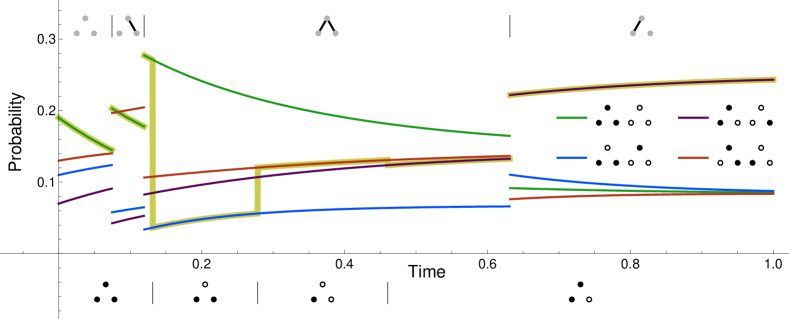
Figure 7: Temporal evolution of the probabilities of all community assignments $\phi$ for $\mathcal{H}(3,2,1,3,1,1,3)$

5.2 Marginalization

Using notation similar to that in Section 3.1, let $p_{i}^{v}(t)\doteq\mathrm{Pr}(\Phi_{t}(v)=i|\mathrm{K}_{[0,t]}=\kappa_{[0,t]})$ be the probability that node $v$ is in community $i$ at time $t$, $p_{ij}^{vw}(t)\doteq\mathrm{Pr}(\Phi_{t}(v)=i,\Phi_{t}(w)=j|\mathrm{K}_{[0,t]}=\kappa_{[0,t]})$, and so on. Note that the same notation $p_{i}^{v}(t)$ was used in Step 1 of the derivation in the previous section to denote a prior probability, but henceforth it will indicate a quantity conditioned on the graph data $\mathrm{K}[0,t]$. To indicate conditioning on $\mathrm{K}[0,t)$ we will use the notation $t^{-}$: e.g., $p_{i}^{v}(t^{-})\doteq\mathrm{Pr}(\Phi_{t}(v)=i|\mathrm{K}_{[0,t)}=\kappa_{[0,t)})$. The prediction and update equations for the full probability distribution are linear (up to a constant factor), so we can sum them over the groups of all nodes aside from $v$ to obtain an expression for $p_{i}^{v}(t)$. When we apply this marginalization to (5.13), we get a quantity $\tilde{p}_{i}^{v}(t)$ proportional to $p_{i}^{v}(t)$ (note that this use of the notation $\tilde{p}_{i}^{v}$ differs from that of Section 3.1). We let $\kappa\doteq\kappa_{t}$ be a concise notation for the graph at time $t$. The marginalization of (5.13) is then

$$\dot{\tilde{p}}_{i}^{v}=\sum_{\iota=1}^{m}a_{i\iota}\tilde{p}_{\iota}^{v}+\sum_{w\in[n]\atop w\neq v}\sum_{j=1}^{m}b_{ij,\kappa(\{v,w\})\kappa(\{v,w\})}\tilde{p}_{ij}^{vw}+\!\!\!\sum_{\{w,x\}\subseteq[n]\atop w,x\neq v}\sum_{j=1}^{m}\sum_{k=1}^{m}b_{jk,\kappa(\{w,x\})\kappa(\{w,x\})}\tilde{p}_{ijk}^{vwx}.$$ (5.16)

We may convert this to an equation for $p_{i}^{v}(t)$ itself (albeit a nonlinear one) by expressing $p_{i}^{v}$ as $p_{i}^{v}(t)=\tilde{p}_{i}^{v}(t)/P_{\kappa}(t)$. The sum of $p_{i}^{v}(t)$ from $i=1$ to $m$ equals 1 for every node $v$, so the sum of $\tilde{p}_{i}^{v}(t)$ from $i=1$ to $m$ is $P_{\kappa}(t)$ for every $v$. Because $\dot{p}_{i}^{v}(t)=\dot{\tilde{p}}_{i}^{v}(t)/P_{\kappa}(t)-p_{i}^{v}(t)S_{\kappa}(t)$, where $S_{\kappa}(t)\doteq\dot{P}_{\kappa}(t)/P_{\kappa}(t)$, we have

$$\begin{split}\dot{p}_{i}^{v}=&-p_{i}^{v}S_{\kappa}+\\ &\sum_{\iota=1}^{m}a_{i\iota}p_{\iota}^{v}+\sum_{w\in[n]\atop w\neq v}\sum_{j=1}^{m}b_{ij,\kappa(\{v,w\})\kappa(\{v,w\})}p_{ij}^{vw}+\!\!\!\sum_{\{w,x\}\subseteq[n]\atop w,x\neq v}\sum_{j=1}^{m}\sum_{k=1}^{m}b_{jk,\kappa(\{w,x\})\kappa(\{w,x\})}p_{ijk}^{vwx}.\end{split}$$ (5.17)

Here $S_{\kappa}$ may be expressed as

$$S_{\kappa}(t)=\!\!\!\sum_{\{v,w\}\subseteq[n]}\sum_{i=1}^{m}\sum_{j=1}^{m}b_{ij,\kappa(\{v,w\})\kappa(\{v,w\})}p_{ij}^{vw}(t).$$ (5.18)

We now marginalize the update equation (5.15) when the edge $e$ transitions from type $l=\kappa_{t^{-}}(e)$ to type $l^{\prime}=\kappa_{t}(e)$. To get the updated probability $p_{i}^{v}(t)$ that node $v$ is in community $i$ after the transition there are two cases: $v\in e$ (say, $e=\{v,w\}$) and $v\notin e$ (say $e=\{w,x\}$):

$$p_{i}^{v}(t)=\frac{1}{S_{l^{\prime}l}(t^{-})}\begin{cases}\displaystyle\sum_{j=1}^{m}b_{ij,l^{\prime}l}p_{ij}^{vw}(t^{-})&\text{if}\;\;e=\{v,w\},\\ \displaystyle\sum_{j=1}^{m}\sum_{k=1}^{m}b_{jk,l^{\prime}l}p_{ijk}^{vwx}(t^{-})\quad&\text{if}\;\;e=\{w,x\}.\end{cases}$$ (5.19)

The normalization constant $S_{l^{\prime}l}(t^{-})$ is independent of the node $v$:

$$S_{l^{\prime}l}(t^{-})=\sum_{i=1}^{m}\sum_{j=1}^{m}b_{ij,l^{\prime}l}p_{ij}^{e_{1}e_{2}}(t^{-}).$$ (5.20)

Whereas the Bayesian filter (5.14) and (5.15) specifies the exact evolution of probabilities in an unmanageably large state space ($m^{n}$ elements), the marginalized filter (5.17) and (5.19) involves only $mn$ elements. It is still an exact filter—no approximations have been made—but it is not useful as it stands because it is not closed. The equations for the first-order statistics $p_{i}^{v}$ involve second- and third-order statistics $p_{ij}^{vw}$ and $p_{ijk}^{vwx}$. One could write down equations for these, but they would involve still higher-order statistics, and so on. Instead, a closure model is needed for the second- and third-order statistics in terms the $p_{i}^{v}$. The topic of closures is discussed in Section 6.

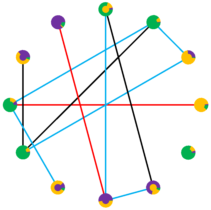
Figure 8: First-order marginals for community membership

To verify (5.17) and (5.19), one can run the full filter (5.14) and (5.15) and use it to compute the required second- and third-order statistics. The results of evolving $p_{i}^{v}(t)$ using these oracular terms should then agree with those obtained by marginalizing the full solution direction. Figure 8 shows the results of such a verification. A simulation of $\mathcal{H}(n,A,\mathbf{B})$ with $n=12$ nodes, $m=3$ communities, and $r=4$ edge types was used to generate graph data $\kappa_{[0,0.8]}$ and ground-truth community assignment data $\phi_{[0,0.8]}$. The transition rate matrices $A$ and $B_{ij}$ used are given in [24]. The final frame $(\phi_{0.8},\kappa_{0.8})$ of this run is shown in Figure 8: the centers of each disk correspond to the communities (green, yellow, or purple) which $\phi_{0.8}$ assigns to each node; the colors of each edge (white, black, blue, or red) are given by $\kappa_{0.8}$. The same parameters $A$ and $\mathbf{B}$ were then used in the Bayesian filter (5.14) and (5.15), which required evolving a system of $3^{12}\approx 530,000$ quantities. The marginalized probabilities $p_{i}^{v}(0.8)$ are depicted in the outer bands, so accuracy is indicated by the outer band largely agreeing with the center.

In the case of the dynamic planted partition model $\mathcal{H}(n,m,a,\lambda_{I},\mu_{I},\lambda_{O},\mu_{O})$, the first-order statistics are trivial: the prediction and update equations reduce to the observation that the probability a node $v$ is in some community equals 1. Instead, with some bookkeeping, one can derive a Bayesian filter for the second-order statistics $p_{ij}^{vw}(t)$ and reduce these to a filter for the co-membership probabilities $p^{\{v,w\}}(t)$: this is similar to what was done in Section 3.2, although that was for an approximation based on limited graph evidence, and this is exact. The filter for $p^{\{v,w\}}$ depends on third- and fourth-order statistics. There are 5 third-order statistics, which sum to 1, and we denote them $p^{\{v\}\{w\}\{x\}}$, $p^{\{v\}\{w,x\}}$, $p^{\{w\}\{v,x\}}$, $p^{\{x\}\{v,w\}}$, and $p^{\{v,w,x\}}$. These correspond to the probabilities that $v$, $w$, and $x$ are in different communities, that two are in the same community with $v$, $w$, and $x$, respectively, being in another, and that all three are in the same community. Similarly there are 15 fourth-order statistics. The two that matter here are $p^{\{v,w,x,y\}}$ and $p^{\{v,w\}\{x,y\}}$. The sum of these two is the probability that $v$ is in the same community as $w$ and that $x$ is in the same community as $y$.

The prediction step of the Bayesian filter for $p^{\{v,w\}}(t)$ may be expressed as

$$\dot{p}^{\{v,w\}}=\frac{2am}{m-1}\left(\frac{1}{m}-p^{\{v,w\}}\right)-\gamma^{vw}q_{vw}^{vw}-\overbrace{\sum_{x\in[n]\atop x\neq v,w}\!\big{(}\gamma^{vx}r_{vw}^{vx}+\gamma^{wx}r_{vw}^{wx}\big{)}}^{\displaystyle R_{vw}}-\,\overbrace{\!\!\!\sum_{\{x,y\}\subseteq[n]\atop x,y\neq v,w}\!\!\!\gamma^{xy}s_{vw}^{xy}}^{\displaystyle S_{vw}}.$$ (5.21)

The form of the update step for $p^{\{v,w\}}$ depends on whether the edge $e$ that is flipping at time $t$ has 2, 1, or 0 nodes in common with $\{v,w\}$:

$$p^{\{v,w\}}(t)=p^{\{v,w\}}(t^{-})+\frac{1}{\delta^{e_{1}e_{2}}(t^{-})}\begin{cases}\gamma_{t^{-}}^{vw}q_{vw}^{vw}(t^{-})&\text{if}\;e=\{v,w\},\\ \gamma_{t^{-}}^{wx}r_{vw}^{wx}(t^{-})&\text{if}\;e=\{w,x\},\\ \gamma_{t^{-}}^{xy}s_{vw}^{xy}(t^{-})&\text{if}\;e=\{x,y\}.\end{cases}$$ (5.22)

The notation used in (5.21) and (5.22) is defined as follows. We define $\gamma_{I,t}^{vw}$ to be the transition rate for an edge to flip (i.e., turn on or off) between nodes $v$ and $w$ at time $t$ under the hypothesis that they are in the same community. This transition rate depends on whether there is currently an edge between $v$ and $w$. Therefore, $\gamma_{I,t}^{vw}$, and its counterpart $\gamma_{O,t}^{vw}$ for the hypothesis that $v$ and $w$ are in different communities, are given by

$$\gamma_{I,t}^{vw}\doteq\begin{cases}\mu_{I}&\text{if}\;\{v,w\}\in E(G_{t}),\\ \lambda_{I}&\text{if}\;\{v,w\}\in E(G_{t}),\end{cases}\quad\text{and}\quad\gamma_{O,t}^{vw}\doteq\begin{cases}\mu_{O}&\text{if}\;\{v,w\}\in E(G_{t}),\\ \lambda_{O}&\text{if}\;\{v,w\}\in E(G_{t}).\end{cases}$$ (5.23)

The quantity $\gamma_{t}^{vw}$, which plays an important role in (5.21) and (5.22), is the difference between the flip rates under the two hypotheses:

$$\gamma_{t}^{vw}\doteq\gamma_{I,t}^{vw}-\gamma_{O,t}^{vw}.$$ (5.24)

On the other hand, the normalization constant $\delta^{vw}(t)$ in (5.22) is the expected flip probability given our current knowledge of the probabilities of the two hypotheses:

$$\delta^{vw}(t)\doteq\gamma_{I,t}^{vw}p^{\{v,w\}}(t)+\gamma_{O,t}^{vw}p^{\{v\}\{w\}}(t),$$ (5.25)

where $p^{\{v\}\{w\}}=1-p^{\{v,w\}}$ is the probability of $v$ and $w$ being in different communities. Finally, the $q$, $r$, and $s$ quantities represent modified second-, third-, and fourth-order statistics, respectively:

$$q_{vw}^{vw} \doteq p^{\{v,w\}}p^{\{v\}\{w\}},$$ (5.26)

$$r_{vw}^{vx} \doteq p^{\{v,w,x\}}-p^{\{v,w\}}p^{\{v,x\}},\;\;\text{and}$$ (5.27)

$$s_{vw}^{xy} \doteq p^{\{v,w,x,y\}}+p^{\{v,w\}\{x,y\}}-p^{\{v,w\}}p^{\{x,y\}}.$$ (5.28)

The $r$ and $s$ quantities measure deviations from independence. That is, if the event $\Phi_{t}(v)=\Phi_{t}(w)$ (i.e., $v$ and $w$ are in the same group at time $t$) were independent of $\Phi_{t}(v)=\Phi_{t}(x)$, then the probability of both events occurring (i.e., $\Phi_{t}(v)=\Phi_{t}(w)=\Phi_{t}(x)$) would equal the product of their probabilities: that is, $p^{\{v,w,x\}}=p^{\{v,w\}}p^{\{v,x\}}$, or $r_{vw}^{vx}=0$. Similarly, if $v$ and $w$ being in the same community were independent of $x$ and $y$ being in the same community (which seems more plausible), then we would have $s_{vw}^{xy}=0$. The terms $R_{vw}$ and $S_{vw}$ represent the accumulated effects on $\dot{p}^{\{v,w\}}$ of the third- and fourth-order deviations from independence, respectively. Understanding the role of these quantities is important for developing an effective closure for this marginalized filter.

6 Community Tracking: Approximation

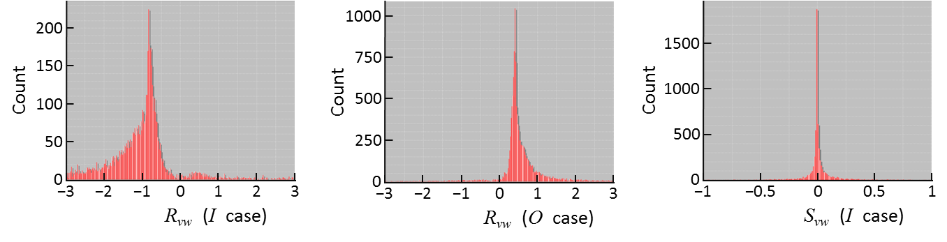
Figure 9: Histograms of third- and fourth-order statistics

To develop closures for the $r_{vw}^{vx}$ and $s_{vw}^{xy}$ terms in (5.21) and (5.22) it helpful to know how they behave statistically. In this section we present a preliminary investigation of these statistics and a possible closure for them using, as an example, the $\mathcal{H}(12,3,0.5,16,4,2,18)$ case depicted in Figure 6. For this case we compute histograms for the $R_{vw}$ and $S_{vw}$ terms in (5.21). In each case, we compile separate histograms for the case of $v$ and $w$ being in the same ground-truth community (case $I$) and in different communities (case $O$). The histograms for the $I$ and $O$ cases of $R_{vw}$ are shown in Figure 9. In the $I$ case, we tend to have $R_{vw}<0$, which makes a positive contribution to $\dot{p}^{\{v,w\}}$ in (5.21); whereas in the $O$ case the opposite occurs. Thus these third-order statistics make an important contribution to the evolution of $p^{\{v,w\}}$. On the other hand, $S_{vw}$ appears to be much less important. In the $I$ case, also shown in Figure 9, $S_{vw}$ is tightly and symmetrically clustered near 0. The $O$ case is similar. This makes sense intuitively: as mentioned at the end of Section 5.2, it seems more plausible for $v$ and $w$ being in the same community to be independent of $x$ and $y$ being in the same community than for $v$ and $w$ to be independent of $v$ and $x$. Therefore, we will make this independence assumption to obtain the fourth-order closure $s_{vw}^{xy}=0$. It remains to develop a closure for $r_{vw}^{vx}$.

The five third-order statistics must sum to one and be consistent with the second-order statistics. This is expressed by the following four equations:

$$p^{\{v\}\{w\}\{x\}}+p^{\{v\}\{w,x\}}+p^{\{w\}\{v,x\}}+p^{\{x\}\{v,w\}}+p^{\{v,w,x\}} =1,$$ (6.1)

$$p^{\{v\}\{w,x\}}+p^{\{v,w,x\}} =p^{\{w,x\}},$$ (6.2)

$$p^{\{w\}\{v,x\}}+p^{\{v,w,x\}} =p^{\{v,x\}},\;\;\text{and}$$ (6.3)

$$p^{\{x\}\{v,w\}}+p^{\{v,w,x\}} =p^{\{v,w\}}.$$ (6.4)

This leaves one degree of freedom, which we choose $p^{\{v,w,x\}}$ to represent. The constraint that the variables in (6.1)–(6.4) are non-negative imposes the following bounds on $p^{\{v,w,x\}}$:

$$p^{-} \doteq\frac{1}{2}\big{(}p^{\{w,x\}}+p^{\{v,x\}}+p^{\{v,w\}}\big{)},\;\;\text{and}$$ (6.5)

$$p^{+} \doteq\min\big{(}p^{\{w,x\}},p^{\{v,x\}},p^{\{v,w\}}\big{)}.$$ (6.6)

For consistency, a closure for $p^{\{v,w,x\}}$ should satisfy $p^{-}\leq p^{\{v,w,x\}}\leq p^{+}$. We will consider closure models that select $p^{\{v,w,x\}}\in[p^{-},p^{+}]$ as a function of $p^{\{w,x\}}$, $p^{\{v,x\}}$, and $p^{\{v,w\}}$. Many natural approximations (such as a symmetric version of $p^{\{v,w,x\}}\approx p^{\{v,w\}}p^{\{v,x\}}$) fail to satisfy $p^{-}\leq p^{\{v,w,x\}}\leq p^{+}$. The approximations $p^{\{v,w,x\}}\approx p^{+}$ and $p^{\{v,w,x\}}\approx p_{0}^{-}\doteq\max(p^{-},0)$ have poor properties. A least-squares solution is possible, but a better principle to employ is maximum entropy [38].

When applying the maximum entropy principle, one needs a suitable underlying measure space. In this discrete case, this simply means a set of atomic events which are equally likely a priori. Such events arise naturally in this case: there are $m^{3}$ of them with probabilities equal to $p_{ijk}^{vwx}$. In the absence of graph data, symmetry implies that their probabilities are each $m^{-3}$. Thus the entropy is defined as

$$H=-\sum_{i=1}^{m}\sum_{j=1}^{m}\sum_{k=1}^{m}p_{ijk}^{vwx}\log p_{ijk}^{vwx}.$$ (6.7)

In this symmetric case, the $m^{3}$ values of $p_{ijk}^{vwx}$ take only five distinct values, so we may re-write (6.7) as

$$\begin{split}H=&-p^{\{v\}\{w\}\{x\}}\log\frac{p^{\{v\}\{w\}\{x\}}}{(m)_{3}}-p^{\{v\}\{w,x\}}\log\frac{p^{\{v\}\{w,x\}}}{(m)_{2}}-p^{\{w\}\{v,x\}}\log\frac{p^{\{w\}\{v,x\}}}{(m)_{2}}\,+\\ &-p^{\{x\}\{v,w\}}\log\frac{p^{\{x\}\{v,w\}}}{(m)_{2}}-p^{\{v,w,x\}}\log\frac{p^{\{v,w,x\}}}{m},\end{split}$$ (6.8)

where $(m)_{r}\doteq m!/(m-r)!$ denotes the falling factorial. We may use (6.1)–(6.4) to express the other variables in terms of $p^{\{v,w,x\}}$, then take the derivative of $H$ with respect to $p^{\{v,w,x\}}$. This reduces to

$$\frac{dH}{dp^{\{v,w,x\}}}=\log\left(\frac{(m-2)^{2}}{4(m-1)}\frac{\big{(}p^{\{w,x\}}-p^{\{v,w,x\}}\big{)}\big{(}p^{\{v,x\}}-p^{\{v,w,x\}}\big{)}\big{(}p^{\{v,w\}}-p^{\{v,w,x\}}\big{)}}{p^{\{v,w,x\}}\big{(}p^{\{v,w,x\}}-p^{-}\big{)}^{2}}\right).$$ (6.9)

Provided $p_{0}^{-}<p^{+}$, the function in (6.9) is strictly decreasing from $\infty$ to $-\infty$ on $[p_{0}^{-},p^{+}]$, so it has a unique zero within this interval, and this zero is where $H$ attains its maximal value on $[p_{0}^{-},p^{+}]$. Finding this zero involves solving a cubic equation, which yields the maximum entropy closure for $r_{vw}^{vx}$.

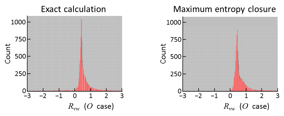
Figure 10: Third-order statistics: exact vs. closure

Figure 10 indicates how well this closure performed in the $\mathcal{H}(12,3,0.5,16,4,2,18)$ example. The histograms show good agreement: each has values that are predominantly positive, with a peak in the same place, and distributions of similar shapes, although the closure distribution is a little more spread out. This suggests that using this closure for $r_{vw}^{vx}$ along with the fourth-order closure $s_{vw}^{xy}$ is a promising idea. Unfortunately, this closure has nothing built into it that ensures $p^{\{v,w\}}$ stays in the range $[0,1]$, and, indeed numerical simulations that use it quickly produce probabilities outside this range.

To see why it fails, consider the consistency requirement $p^{-}\leq p^{+}$ mentioned above. This may be re-written

$$\big{|}p^{\{v\}\{x\}}-p^{\{w\}\{x\}}\big{|}\leq p^{\{v\}\{w\}}\leq p^{\{v\}\{x\}}+p^{\{w\}\{x\}},$$ (6.10)

i.e., the probabilities $p^{\{v\}\{w\}}$ satisfy the triangle inequality. In particular, if $p^{\{v,w\}}=1$, then $p^{\{v,x\}}=p^{\{w,x\}}$ for all nodes $x\neq v,w$. This makes sense: if $v$ and $w$ are definitely in the same community $C$, then both $p^{\{v,x\}}$ and $p^{\{w,x\}}$ mean “the probability that $x\in C$,” so it would be illogical for these values to differ. Furthermore, in the special case $a=0$, if $p^{\{v,w\}}=1$ at some time, then it will remain 1, which implies $\dot{p}^{\{v,x\}}=\dot{p}^{\{w,x\}}$. The direct verification of this fact using (5.21) leads to an expression in which $S_{vw}=-R_{vw}\neq 0$. In this case, the fourth-order terms play a crucial role in maintaining consistency, so it is not surprising truncating them entirely leads to inconsistencies. This is but one of the issues that must be addressed before principled community tracking algorithms along these lines can be developed, but we believe there is much promise in this approach of Bayesian filtering using formal evolution and measurement models

7 Conclusion

Network science has benefited from the perspectives and expertise of a variety of scientific communities. The data fusion approach has much to offer as well. It provides an integrated framework for synthesizing high-level situational awareness from messy, real-world data. It also develops tracking algorithms based on formal evolution models that maintain representations of the uncertainty of the ground-truth state. We have applied this perspective to the community detection problem in network science. We began with a derivation of the posterior probability distribution of community structure given some graph data: this is similar to the approach of [33, 34]. However, rather than seeking the community structure that maximizes this posterior probability, we developed approximations to the marginals of these distributions. In particular, we consider the pairwise co-membership probability $p^{\{v,w\}}$: the probability that nodes $v$ and $w$ are in the same community. We develop an estimate of $p^{\{v,w\}}$ based on using limited information from the graph $G$ and approximating an integral over the model’s structural parameters. The resulting method is very fast, and, when exploited to produce a single community detection result (via the utility formulation in Appendix A) yields state-of-the-art accuracy. Various uses for these $p^{\{v,w\}}$ quantities are combined in the network analysis and visualization product IGNITE.

We extended our community detection approach to tracking the evolution of time-varying communities in time-varying graph data. We proposed dynamic analogs of the stochastic blockmodel and planted partition models used in static community detection: these models are continuous-time Markov processes for the joint evolution of the communities and the graph. We derived a Bayesian filter for the current probability distribution over all community structures given the previous history of the graph data. This filter decomposes into prediction steps (during periods of constant graph data) and update steps (at times when the graph changes). The filter is over too large a state space to use directly, so we marginalized it to get state spaces of a reasonable size. These marginalized equations require closures for their higher-order terms, and we discussed one possible closure based on maximum entropy.

The community detection work could be extended to more realistic graph models, such as the degree-corrected blockmodel of [41], and the integral approximation developed in Section 3.2 could certainly be improved. There is much more work to do in the community tracking case, however. In the spectrum of methods that handle dynamic network data, the models presented are intermediate between those that use the data only to discern a static community structure (e.g., [67]) and those mentioned in Section 5 that allow not just individual node movements, but the birth, death, splitting, and merging of communities. Extending this methodology to account for these phenomena would be important for applications. Whatever model is used, some method for parameter selection must be developed. Integrating over the parameter space may be too complicated in the community tracking case, but one may be able to extend the Bayesian filter by making the input parameters themselves hidden variables, and use Hidden Markov Model (HMM) techniques for parameter learning [4]. Closures must be developed, preferably with proofs of their properties, rather than just experimental justification. Finally, to be truly useful, community tracking need to be able to incorporate ancillary, non-network information about the properties of the nodes and edges involved. Bayesian data fusion provides an excellent framework for coping with this kind of practical problem by identifying what expert knowledge is needed to extend the uncertainty management in a principled manner.

Appendix A Expected Utility Formulation

Figure 11 depicts the data fusion approach this paper takes toward community detection and tracking. Part (1) represents the model of the hidden state space in which we are interested (in this case the community assignments $\phi$ or community partitions $\pi$), including some prior probability distribution over it, and, in the dynamic case, an evolution model. Part (2) represents observed data, and the red arrow from (1) to (2) is the measurement model which assigns conditional probabilities of the data given the true state. Part (3) is Bayesian inversion, which yields the conditional probabilities of the true state given the data. When the number of possible states is large, the combinatorial explosion of part (3) must be dealt with in some manner. Thus, part (4) is some reduced representation of the full posterior distribution in (3): in this case the pairwise co-membership probabilities $p^{\{v,w\}}$. Finally, part (5) represents the end user of this inference process. The full posterior could, in principle, answer every question the end user might have about the true state, given the limitation of the data available. The reduced representation (4) should be chosen in such a way that it may be gleaned efficiently from (3), but also meet the needs of the end user (5).

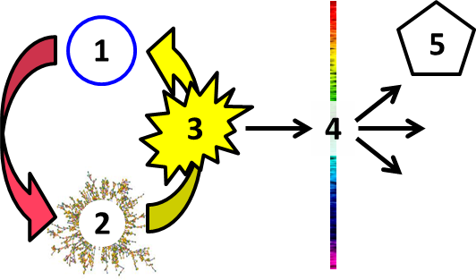
Figure 11: Five-part inference framework

The body of this paper addresses parts (1)–(4) for the community detection and tracking problems. This appendix connects that analysis to part (5). Bayesian decision theory [5] provides a way to formalize the connection. Consider the problem of how to assess the quality of some proposed (or computed) partition $\hat{\pi}$. The usual approach is to stipulate some quality function of $\hat{\pi}$ and the graph $G$. Bayesian decision theory argues for assessing the quality of $\hat{\pi}$ in terms of its agreement with the true partition $\pi$. Thus, with the cooperation of the end user in (5), we should construct a utility function $U(\hat{\pi}|\pi)$ which defines the value of being provided the answer $\hat{\pi}$ when the true partition is $\pi$. Because the ground truth partition $\pi$ is unknown, we cannot compute $U(\hat{\pi}|\pi)$. However, if we know the posterior distribution $\mathrm{Pr}(\pi|G)$, we can compute the expected utility $\mathbb{E}[U](\hat{\pi}|G)$. In general, summing over all possible partitions $\pi$ to get this expected utility is not practical, but we shall provide a generic example in which the summation reduces to one over all pairs of nodes, with the set of pairwise co-membership probabilities $p^{\{v,w\}}$ providing all necessary statistical information. In this sense, the values of $p^{\{v,w\}}$ comprise the reduced representation in part (4) of Figure 11.

Let $V=[n]$ denote the set of $n$ nodes, and $\Pi(V)$ denote the set of all partitions of $V$. For any particular $\pi\in\Pi(V)$, let $U(\hat{\pi}|\pi)$ denote the utility of the decision that $\hat{\pi}$ is the correct partition when $\pi$ is in fact correct. For any graph $G$ on $V$, one may define the quality of $\hat{\pi}$ for $G$ to be the expected value of its utility:

$$\mathbb{E}[U](\hat{\pi}|G)=\!\!\sum_{\pi\in\Pi(V)}\!\!U(\hat{\pi}|\pi)\mathrm{Pr}(\pi|G),$$ (A.1)

where $\mathrm{Pr}(\pi|G)$ is the posterior probability of $\pi$ given $G$. To simplify (A.1), assume $U(\hat{\pi}|\pi)$ is additive: i.e., that it can be expressed as

$$U(\hat{\pi}|\pi)=\sum_{\hat{C}\in\hat{\pi}}u(\pi[\hat{C}])$$ (A.2)

for some function $u$, where $\pi[\hat{C}]$ is the partition of $\hat{C}$ induced by $\pi$ (that is, the sets into which $\pi$ “chops up” $\hat{C}$). In this case, one can compute the expected utility of each community $\hat{C}\in\hat{\pi}$ given $G$,

$$\mathbb{E}[U](\hat{C}|G)=\!\!\sum_{\pi\in\Pi(V)}\!\!u(\pi[\hat{C}])\mathrm{Pr}(\pi|G),$$ (A.3)

and sum them over $\hat{C}\in\hat{\pi}$ afterward to get $\mathbb{E}[U](\hat{\pi}|G)$. Grouping the sum in (A.3) into classes based on the value of $\pi[\hat{C}]$ yields

$$\mathbb{E}[U](\hat{C}|G)=\!\!\sum_{\rho\in\Pi(\hat{C})}\!\!u(\rho)\!\!\!\!\sum_{\pi:\pi[\hat{C}]=\rho}\!\!\!\mathrm{Pr}(\pi|G).$$ (A.4)

The inner sum in (A.4) is the probability of $\rho$ given $G$, denoted $\mathrm{Pr}(\rho|G)$. By grouping the sum in (A.3) less aggressively, however, one obtains a more general result which includes (A.3) and (A.4) as special cases. For any $\hat{C}^{+}\supseteq\hat{C}$,

$$\mathbb{E}[U](\hat{C}|G)=\!\!\!\!\sum_{\rho^{+}\in\Pi(\hat{C}^{+})}\!\!\!\!u(\rho^{+}[\hat{C}])\mathrm{Pr}(\rho^{+}|G).$$ (A.5)

In particular, we let $\hat{C}^{+}=\hat{C}\cup\{v\}$ and define

$$\delta(\hat{C},v)=\mathbb{E}[U](\hat{C}^{+}|G)-\mathbb{E}[U](\hat{C}|G)-\mathbb{E}[U](\{v\}|G)$$ (A.6)

to be the increase in expected utility of merging the community $\hat{C}$ with the singleton community $\{v\}$. Using (A.5), $\delta(\hat{C},v)$ may be expressed as

$$\delta(\hat{C},v)=\!\!\!\!\sum_{\rho^{+}\in\Pi(\hat{C}^{+})}\!\!\!\!\left(u(\rho^{+})-u(\rho^{+}[\hat{C}])-u(\{\{v\}\})\right)\mathrm{Pr}(\rho^{+}|G).$$ (A.7)

This equation allows the expected utility of a community to be computed by adding one node at a time.

A.1 A generic utility model

Here we consider a simple, generic utility function in which some node $v$ has been identified as “bad,” implying that the nodes in his ground-truth community $C=\pi(v)$ are bad as well, but that decision makers are using some other partition $\hat{\pi}$, resulting in all nodes in $\hat{C}=\hat{\pi}(v)$ ending up “dead.” Let $u_{BD}$ and $u_{BA}$ be the respective utilities of a bad node being dead and being alive, and $u_{GD}$ and $u_{GA}$ be the corresponding utilities for good nodes. Summing the utilities over the cases $v\in V$ being identified as bad yields the utility function

$$\begin{split}U^{*}(\hat{\pi}|\pi)=&(u_{BD}-u_{BA}-u_{GD}+u_{GA})\!\!\!\sum_{C\in\pi,\hat{C}\in\hat{\pi}}\!\!\!\!|C\cap\hat{C}|^{2}+\\ &(u_{BA}-u_{GA})\sum_{C\in\pi}|C|^{2}+(u_{GD}-u_{GA})\sum_{\hat{C}\in\hat{\pi}}|\hat{C}|^{2}+u_{GA}n^{2}\end{split}$$ (A.8)

after some rearrangement. Assuming $u_{GA}\geq u_{GD}$ and $u_{BD}\geq u_{BA}$ (and equality does not hold for both), a convenient choice of translation and scaling yields

$$U(\hat{\pi}|\pi)=\frac{1}{2}\bigg{(}\;\sum_{C\in\pi,\hat{C}\in\hat{\pi}}\!\!\!\!|C\cap\hat{C}|^{2}-\theta\sum_{\hat{C}\in\hat{\pi}}|\hat{C}|^{2}-(1-\theta)n\bigg{)},$$ (A.9)

where the threshold $\theta=(u_{GA}-u_{GD})/(u_{GA}-u_{GD}+u_{BD}-u_{BA})\in[0,1]$ reflects the emphasis of killing bad nodes (small $\theta$, yielding large communities) versus not killing good nodes (large $\theta$, small communities). This utility function is additive: it may be decomposed according to (A.2) with

$$u(\rho)=\frac{1}{2}\bigg{(}\;\sum_{C\in\rho}|C|^{2}-\theta|\hat{C}|^{2}-(1-\theta)|\hat{C}|\bigg{)},$$ (A.10)

for any $\rho\in\Pi(\hat{C})$. Note that $u(\rho)=0$ for singleton partitions $\rho=\{\{v\}\}$.

Substituting into (A.10) into (A.7) yields

$$\delta(\hat{C},v)=\!\!\!\sum_{\rho^{+}\in\Pi(\hat{C}^{+})}\!\!\Big{(}|\rho^{+}(v)|-1-\theta|\hat{C}|\Big{)}\mathrm{Pr}(\rho^{+}|G).$$ (A.11)

This may be written $\delta(\hat{C},v)=\mathbb{E}[\rho^{+}(v)-1|G]-\theta|\hat{C}|$. The first term here is the expected number of nodes in $\hat{C}$ that are in the same community as $v$ in a random partition of $\hat{C}^{+}$, given the evidence $G$. Linearity of expectation implies

$$\mathbb{E}[\rho^{+}(v)-1|G]=\sum_{w\in\hat{C}}p^{\{v,w\}},$$ (A.12)

where $p^{\{v,w\}}=\mathrm{Pr}(\{\{v,w\}\}|G)$ is the probability that $v$ and $w$ lie in the same community, given $G$. This may be used to build up $\mathbb{E}[U](\hat{C}|G)$ by adding nodes $v$ to $\hat{C}$ one at a time, which yields the simple formula

$$\mathbb{E}[U](\hat{C}|G)=\!\!\!\sum_{\{v,w\}\subseteq\hat{C}}\!\!\!\big{(}p^{\{v,w\}}-\theta\big{)}.$$ (A.13)

Summing this over $\hat{C}$ yields an expression for the expected utility of a partition $\hat{\pi}$ given the graph $G$ which involves only sums over pairs of nodes in the same community $\hat{C}\in\hat{\pi}$:

$$\mathbb{E}[U](\hat{\pi}|G)=\!\sum_{\hat{C}\in\hat{\pi}}\!\!\sum_{\{v,w\}\subseteq\hat{C}}\!\!\!\big{(}p^{\{v,w\}}-\theta\big{)}.$$ (A.14)

References

- [1] E. Airoldi, D. M. Blei, S. E. Fienberg, A. Goldenberg, E. P. Xing, and A. X. Zheng (eds.), Statistical network analysis: Models, issues, and new directions, Springer, 2007.
- [2] Y. Bar-Shalom, P. K. Willett, and X. Tian, Tracking and data fusion: A handbook of algorithms, Yaakov Bar-Shalom, 2011.
- [3] W. F. Basener, B. P. Brooks, and D. Ross, Brouwer fixed point theorem applied to rumour transmission, Applied Mathematics Letters 19 (2006), no. 8, 841–842.
- [4] L. E. Baum and T. Petrie, Statistical inference for probabilistic functions of finte state Markov chains, Annals of Mathematical Statistics 37 (1966), 1554–1563.
- [5] J. O. Berger, Statistical decision theory and bayesian analysis, Springer, 1993.
- [6] I. Bhattacharya and L. Getoor, Entity resolution in graphs, Mining Graph Data (D. J. Cook and L. B. Holder, eds.), John Wiley & Sons, Inc., Hoboken, NJ, 2006.
- [7] E. Blasch, I. Kadar, J. Salerno, M. M. Kokar, S. Das, G. M. Powell, D. D. Corkill, and E. H. Ruspini, Issues and challenges in situation assessment (level 2 fusion), J. Advances Information Fusion 1 (2006), no. 2, 122–139.
- [8] V. D. Blondel, J.-L. Guillaume, R. Lambiotte, and E. Lefebvre, Fast unfolding of communities in large networks, J. Stat. Mech. (2008), P10008.
- [9] B. Bollobás, Modern graph theory, Springer, New York, 1998.
- [10] , Random graphs, Cambridge University Press, New York, 2001.
- [11] N. A. Christakis and J. H. Fowler, The spread of obesity in a large social network over 32 years, New England Journal of Medicine 357 (2007), 370–379.
- [12] A. Clauset, C. Moore, and M. E. J. Newman, Hierarchical structure and the prediction of missing links in networks, Nature 453 (2008), 98–101.
- [13] V. Colizza, R. Pastor-Satorras, and A. Vespignani, Reaction–diffusion processes and metapopulation models in heterogeneous networks, Nature Physics 3 (2007), 276–282.
- [14] A. Condon and R. M. Karp, Algorithms for graph partitioning on the planted partition model, Random Structures and Algorithms 18 (2001), no. 2, 116–140.
- [15] T. H. Cormen, C. E. Leiserson, R. L. Rivest, and C. Stein, Introduction to algorithms, third ed., MIT Press, 2009.
- [16] D. R. Cox and H. D. Miller, The theory of stochastic processes, Chapman & Hall/CRC, 1965.
- [17] D. F. Crouse, P. Willett, and Y. Bar-Shalom, Generalizations of Blom and Bloem’s PDF decomposition for permutation-invariant estimation, Proceedings of the IEEE International Conference on Acoustics, Speech, and Signal Processing, ICASSP, 2011, pp. 3840–3843.
- [18] P. Daniele, Dynamic networks and evolutionary variational inequalities, Edward Elgar Publishing, 2006.
- [19] T. A. Davis and Y. Hu, The University of Florida sparse matrix collection.
- [20] P. Doreian, V. Batagelj, and A. Ferligoj, Generalized blockmodeling, Cambridge University Press, New York, 2005.
- [21] P. Doreian and F. N. Stokman (eds.), Evolution of social networks, Routledge, 1997.
- [22] M. Feldmann, D. Fränken, and W. Koch, Tracking of extended objects and group targets using random matrices, IEEE Transactions on Signal Processing 59 (2011), no. 4, 1409–1420.
- [23] D. J. Fenn, M. A. Porter, M. McDonald, S. Williams, N. F. Johnson, and N. S. Jones, Dynamic communities in multichannel data: An application to the foreign exchange market during the 2007–2008 credit crisis, Chaos 19 (2009), 033119.
- [24] J. P. Ferry, Group tracking on dynamic networks, Proc. 12th Int. Conf. on Information Fusion, July 2009, pp. 930–937.
- [25] , Exact association probability for data with bias and features, J. Advances Information Fusion 5 (2010), no. 1, 41–67.
- [26] J. P. Ferry and J. O. Bumgarner, Tracking group co-membership on networks, Proc. 13th Int. Conf. on Information Fusion, July 2010.
- [27] J. P. Ferry, J. O. Bumgarner, and S. T. Ahearn, Probabilistic community detection in networks, Proc. 14th Int. Conf. on Information Fusion, July 2011.
- [28] S. Fortunato, Community detection in graphs, Physics Reports 486 (2010), no. 3–5, 75–174.
- [29] L. C. Freeman, The development of social network analysis: A study in the sociology of science, Empirical Press, 2004.
- [30] L. Grady, Random walks for image segmentation, IEEE transactions on pattern analysis and machine intelligence 28 (2006), no. 11, 1768–1783.
- [31] D. Greene, D. Doyle, and P. Cunningham, Tracking the evolution of communities in dynamic social networks., ASONAM’10, 2010, pp. 176–183.
- [32] D. L. Hall, R. Nagi, J. Llinas, J. Lavery, and A. Shirkhodaie, Multidisciplinary research in hard and soft information fusion, Proc. 13th Int. Conf. on Information Fusion, July 2010.
- [33] M. B. Hastings, Community detection as an inference problem, Phys. Rev. E 74 (2006), no. 3, 035102.
- [34] J. M. Hofman and C. H. Wiggins, A Bayesian approach to network modularity, Phys. Rev. Lett. 100 (2008), 258701.
- [35] J. Hopcroft, O. Khan, B. Kulis, and B. Selman, Tracking evolving communities in large linked networks, Proc. Natl. Acad. Sci. USA 101 (2004), no. suppl. 1, 5249–5253.
- [36] A. Jain and R. Dubes, Algorithms for clustering data, Prentice Hall, 1988.
- [37] S. Janson, T. Łuczak, and A. Ruciński, Random graphs, John Wiley & Sons, New York, 2000.
- [38] E. T. Jaynes, Probability theory: The logic of science (vol 1), Cambridge University Press, 2003.
- [39] A. H. Jazwinski, Stochastic processes and filtering, Academic Press, 1970.
- [40] R. E. Kalman, A new approach to linear filtering and prediction problems, Transactions of the ASME—Journal of Basic Engineering, Series D 82 (1960), 35–45.
- [41] B. Karrer and M. E. J. Newman, Stochastic blockmodels and community structure in networks, Phys. Rev. E 83 (2011), no. 1, 016107.
- [42] W. O. Kermack and A. G. McKendrick, A contribution to the mathematical theory of epidemics, Proc. Roy. Soc. Lond. A 115 (1927), 700–721.
- [43] A. Lancichinetti and S. Fortunato, Benchmarks for testing community detection algorithms on directed and weighted graphs with overlapping communities, Phys. Rev. E 80 (2009), no. 1, 016118.
- [44] A. Lancichinetti, S. Fortunato, and J. Kertész, Detecting the overlapping and hierarchical community structure in complex networks, New Journal of Physics 11 (2009), 033015.
- [45] A. Lancichinetti, M. Kivelä, J. Saramäki, and S. Fortunato, Characterizing the community structure of complex networks, PLoS One 5 (2010), no. 8, e11976.
- [46] R. T. A. J. Leenders, Models for network dynamics: A markovian framework, Journal of Mathematical Sociology 20 (1995), no. 1, 1–21.
- [47] J. Leskovec, L. Adamic, and B. Huberman, The dynamics of viral marketing, ACM Transactions on the Web 1 (2007), no. 1, 5–es.
- [48] J. Leskovec, J. Kleinberg, and C. Faloutsos, Graphs over time: Densification laws, shrinking diameters and possible explanations, KDD ’05: Proc. 11th ACM SIGKDD Int. Conf. on Knowledge Discovery and Data Mining (KDD) (New York, NY), ACM Press, 2005.
- [49] J. Leskovec, K. J. Lang, A. Dasgupta, and M. W. Mahoney, Community structure in large networks: Natural cluster sizes and the absence of large well-defined clusters, Internet Mathematics 6 (2009), no. 1, 29–123.
- [50] T. G. Lewis, Network science: Theory and applications, Wiley, 2009.
- [51] M. E. Liggins, D. L. Hall, and J. Llinas (eds.), Handbook of multisensor data fusion, 2nd edition ed., CRC Press, Boca Raton, FL, 2009.
- [52] M. McPherson, L. Smith-Lovin, and J. M. Cook, Birds of a feather: Homophily in social networks, Ann. Rev. Sociology 27 (2001), 415–444.
- [53] S. Mori and C.-Y. Chong, Track-to-track association metric – i.i.d.-non-Poisson cases –, Proc. 6th Int. Conf. on Information Fusion, July 2003.
- [54] B. Nadler, S. Lafon, R. R. Coifman, and I. G. Kevrekidis, Diffusion maps, spectral clustering and eigenfunctions of Fokker–Planck operators, Advances in Neural Information Processing Systems 18 (2005), 955–962.
- [55] M. E. J. Newman, Networks: An introduction, Oxford University Press, USA, 2010.
- [56] M. E. J. Newman and M. Girvan, Finding and evaluating community structure in networks, Phys. Rev. E 69 (2004), 026113.
- [57] M. E. J. Newman and E. A. Leicht, Mixture models and exploratory analysis in networks, Proc. Natl. Acad. Sci. USA 104 (2007), 9564–9569.
- [58] J. M. Ortega, Matrix theory: A second course, Springer, 1987.
- [59] G. Palla, A.-L. Barabási, and T. Vicsek, Quantifying social group evolution, Nature 446 (2007), 664–667.
- [60] G. Palla, I. Derényi, I. Farkas, and T. Vicsek, Uncovering the overlapping community structure of complex networks in nature and society, Nature 435 (2005), 814–818.
- [61] J. Reichardt and S. Bornholdt, Detecting fuzzy community structures in complex networks with a Potts model, Phys. Rev. Lett. 93 (2004), 218701.
- [62] , Statistical mechanics of community detection, Phys. Rev. E 74 (2006), 016110.
- [63] P. Ronhovde and Z. Nussinov, Multiresolution community detection for megascale networks by information-based replica correlations, Phys. Rev. E 80 (2009), no. 1, 016109.
- [64] M. Rosvall and C. T. Bergstrom, Maps of random walks on complex networks reveal community structure, Proc. Natl. Acad. Sci. USA 105 (2008), no. 4, 1118–1123.
- [65] , Mapping change in large networks, PLoS One 5 (2010), no. 1, e8694.
- [66] , Multilevel compression of random walks on networks reveals hierarchical organization in large integrated systems, PLoS One 6 (2011), no. 4, e18209, arXiv:1010.0431v1.
- [67] C. R. Shalizi, M. F. Camperi, and K. L. Klinkner, Discovering functional communities in dynamical networks, in Airoldi et al. [1], pp. 140–157.
- [68] T. A. B. Snijders, G. G. van de Bunt, and C. E. G. Steglich, Introduction to stochastic actor-based models for network dynamics, Social Networks 32 (2010), no. 1, 44–60.
- [69] A. N. Steinberg and C. L. Bowman, Revisions to the JDL data fusion model, in Liggins et al. [51], pp. 45–68.
- [70] L. D. Stone, C. A. Barlow, and T. L. Corwin, Bayesian multiple target tracking, Artech House, Inc., Norwood, MA, USA, 1999.
- [71] R. Sulo, T. Berger-Wolf, , and R. Grossman, Meaningful selection of temporal resolution for dynamic networks, Proc. 8th Workshop on Mining and Learning with Graphs (Washington, DC), ACM Press, July 2010, pp. 127–136.
- [72] C. Tantipathananandh and T. Berger-Wolf, Constant-factor approximation algorithms for identifying dynamic communities, Proc. 15th ACM SIGKDD international conference on knowledge discovery and data mining (Paris, France), ACM Press, July 2009, pp. 827–836.
- [73] C. Tantipathananandh, T. Berger-Wolf, and D. Kempe, A framework for community identification in dynamic social networks, Proc. 13th ACM SIGKDD international conference on knowledge discovery and data mining (San Jose, CA), ACM Press, August 2007, pp. 717–726.
- [74] A. L. Traud, E. D. Kelsic, P. J. Mucha, and M. A. Porter, Comparing community structure to characteristics in online collegiate social networks, to appear in SIAM Review (2011).
- [75] T. W. Valente, Social network thresholds in the diffusion of innovations, Social Networks 18 (1996), 69–89.
- [76] P. K. Varshney, Distributed detection and data fusion, Springer, 1996.
- [77] S. Wasserman and K. Faust, Social network analysis, Cambridge University Press, 1994.
- [78] N. Wiener, Extrapolation, interpolation, and smoothing of stationary time series, Wiley, 1949.
- [79] W. W. Zachary, An information flow model for conflict and fission in small groups, J. Anthropological Research 33 (1977), 445–473.