Majorana neutrino magnetic moments in the gauge mediated supersymmetry breaking MSSM model

Abstract

Supersymmetric models with broken $R$-parity provide mechanisms that allow to generate Majorana neutrino masses and magnetic moments through virtual particle-sparticle loops. This constitutes an attractive alternative to the see-saw mechanism. In this paper we present a detailed calculation of the transition magnetic moments of a Majorana neutrino in gauge mediated supersymmetry breaking MSSM without $R$-parity. We base our analysis on the renormalization group evolution of the MSSM parameters, which are unified at the GUT scale.

I Introduction

After establishing the fact that neutrinos do oscillate nu-osc , the window to physics beyond the Standard Model (SM) has been opened. It is difficult to guess to what extend the already known theory of elementary particles and interactions needs altering. It is customary to believe, however, that the SM should be treated as a low-energy approximation of a more general theory, which will not only work for high energies, thus describing the creation of the Universe, but should also use a unified description of all the interactions, presumably including gravity. A good candidate seems to be somehow connected with the string theory, which in turn requires supersymmetry (as well as additional spatial dimensions) for consistency.

A close cooperation between the development of theory and experiments is essential. Despite the fact that direct testing of these models in the ultra-high energy regime is by now impossible, different models may foresee certain features of some elementary particles, branching ratios and others. These subtle clues, when found in future generation experiments, may lead to favoring some and ruling out the other models, providing an important insight into high-energy exotic physics. One cannot therefore underestimate the importance of study of different theories beyond the SM and their implications.

One of the most promising concepts that extends beyond the SM is supersymmetry (SUSY). It is strongly connected with the string theory, which in order to be able to describe not only interactions (bosonic strings) but also matter (fermionic strings) requires the introduction of SUSY. SUSY provides an elegant way of describing fermionic and bosonic fields grouped in a single supermultiplet, and it is a basic exercise to show that each supermultiplet must consist of equal number of degrees of freedom of both kinds. Therefore, introduction of SUSY unifies in some sense the description of matter and interactions. What is more, the Minimal Supersymmetric Standard Model (MSSM; see mssm ; kazakov and references therein for a review) possesses the attractive feature that the gauge couplings unify at the energy $m_{\rm GUT}\sim 10^{16}$ GeV, which is not true in the ordinary SM. It is remarkable that in order to go beyond the SM in a consistent way one is forced to accept a whole bunch of new ideas like supersymmetry, extra dimensions, grand unification (GUT) and others. The problem, however, is that nobody can really state the actual details of these models. For example, supposing that supersymmetry exists, it needs to be broken, as it is not observed in our energy regime. Of course the details of the mechanism of this breaking are not known. The difficulty with extra dimensions is that one needs to justify why they cannot be seen, why do they not open, what is the mechanism of compactification and stabilization. The pattern and mechanism of unification of matter and interactions at $m_{\rm GUT}$ or $m_{\rm Planck}$ can also be only a guess.

As mentioned at the very beginning, the only link we directly investigate, leading beyond the SM, are neutrinos. In spite of the fact that it is a neutral particle, in certain exotic models it may possess non-zero transition magnetic moments (in the case of Majorana neutrinos this is the only possible type of magnetic moment; the Dirac neutrinos may possess the transition as well as the diagonal magnetic moments). This happens in all supersymmetric models in which the so-called $R$-parity is not conserved barbier ; aul83 ; valle ; np ; rbreaking . In principle this feature should leave a clear signature, but the present sensitivities of the experiments are at best five orders of magnitude to weak. The observation of an electromagnetic interaction of the neutrino would be a breakthrough and may give us important information about details of the exotic models.

The problem of generating Majorana neutrino mass and transition magnetic moments in $R$-parity violating MSSM has been widely discussed in the literature Haug ; Bhatta ; Abada ; rpvneutrinos ; mg ; mg-art09 ; mg-art15 . Many older approaches used certain simplifying assumptions about the low-energy mass spectrum of the MSSM model. This has been corrected by the use of GUT conditions and renormalization group equations (RGE) mg ; mg-art09 ; mg-art15 , which made the whole discussion dependent on a few unification parameters only. Up to our best knowledge, all calculations made so far used the supergravity mechanism of supersymmetry breaking.

In this paper we present detailed calculations performed assuming the gauge mediated supersymmetry breaking mechanism, for the whole allowed parameter space. The paper is organized as follows. In the next section we define the model, which is the minimal supersymmetric standard model with gauge mediated supersymmetry breaking and not conserved $R$-parity. In Section III we describe our procedure of obtaining the low-energy spectrum of the model, together with different constraints we impose on the results. Next, we discuss the Majorana neutrino transition magnetic moments and present numerical results. A short conclusion follows at the end.

II RpV MSSM with gauge mediated supersymmetry breaking

The Minimal Supersymmetric Standard Model mssm ; kazakov is a minimal extension of the usual SM which incorporates supersymmetry. It implies that each particle gains a superpartner with spin different by 1/2 unit. There is also an additional Higgs doublet introduced, in order to assign masses to the up- and down-type particles. In result, the number of particles in MSSM roughly doubles that of the SM.

In basic formulation of the MSSM one assumes ad-hoc the conservation of the lepton and baryon numbers. This is achieved by the introduction of an artificial symmetry called the $R$-parity. It is defined as $R=(-1)^{3B+L+2S}$, where $B$ is the baryon number, $L$ the lepton number, and $S$ the spin of the particle. The definition implies that all ordinary SM particles have $R=+1$ and all their superpartners have $R=-1$. In theories preserving $R$-parity the product of $R$ of all the interacting particles in a vertex of a Feynman diagram must be equal to $1$. It follows that a SUSY particle must decay into another SUSY particle, thus the lightest SUSY particle must remain stable and is considered a good candidate for the cold dark matter. In many models this particle is the lightest neutralino, but sometimes the gluino takes its place. In the case of gauge mediated supersymmetry breaking the lightest stable SUSY particle is the gravitino.

The main motivation for the introduction of $R$-parity is the conservation of $L$ and $B$ numbers. However, we already know that at least the flavour lepton numbers $L_{e}$, $L_{\mu}$, and $L_{\tau}$ are not conserved, as has been seen in the neutrino oscillation experiments. There is also a strong suspicion that at higher energies the full $L$ symmetry may not be exact. From formal theoretical point of view, nothing motivates the rejection of interaction terms that do violate the $R$-parity. This leads us to $R$-parity violating (RpV) models, which exhibit richer and more interesting phenomenology.

The full RpV MSSM model is described by the superpotential, which includes the Lagrangian as its $F-$term. It consists of two parts: $W=W^{MSSM}+W^{RpV}$. The $R$-parity conserving part of the superpotential of MSSM is usually written as

$$W^{MSSM} = \epsilon_{ab}[(\mathbf{Y}_{E})_{ij}L_{i}^{a}H_{u}^{b}\bar{E}_{j}+(\mathbf{Y}_{D})_{ij}Q_{ix}^{a}H_{d}^{b}\bar{D}_{j}^{x}$$ (1)

$$+ (\mathbf{Y}_{U})_{ij}Q_{ix}^{a}H_{u}^{b}\bar{U}_{j}^{x}+\mu H_{d}^{a}H_{u}^{b}],$$

while its RpV part reads

$$W^{RpV} = \epsilon_{ab}\left[\frac{1}{2}\lambda_{ijk}L_{i}^{a}L_{j}^{b}\bar{E}_{k}+\lambda^{\prime}_{ijk}L_{i}^{a}Q_{jx}^{b}\bar{D}_{k}^{x}\right]$$ (2)

$$+ \frac{1}{2}\epsilon_{xyz}\lambda^{\prime\prime}_{ijk}\bar{U}_{i}^{x}\bar{D}_{j}^{y}\bar{D}_{k}^{z}+\epsilon_{ab}\kappa^{i}L_{i}^{a}H_{u}^{b}.$$

The Y’s are 3$\times$3 Yukawa matrices. $L$ and $Q$ are the $SU(2)$ left-handed doublets while $\bar{E}$, $\bar{U}$ and $\bar{D}$ denote the right-handed lepton, up-quark and down-quark $SU(2)$ singlets, respectively. $H_{d}$ and $H_{u}$ mean two Higgs doublets. We have introduced color indices $x,y,z=1,2,3$, generation indices $i,j,k=1,2,3=e,\mu,\tau$ and the $SU(2)$ spinor indices $a,b=1,2$.

The mass terms (self-interaction terms) for the Higgs bosons, sfermions, and gauginos take the standard form:

$${\cal L}^{mass} = \mathbf{m}^{2}_{H_{d}}h_{d}^{\dagger}h_{d}+\mathbf{m}^{2}_{H_{u}}h_{u}^{\dagger}h_{u}+q^{\dagger}\mathbf{m}^{2}_{Q}q+l^{\dagger}\mathbf{m}^{2}_{L}l$$

$$+ u\mathbf{m}^{2}_{U}u^{\dagger}+d\mathbf{m}^{2}_{D}d^{\dagger}+e\mathbf{m}^{2}_{E}e^{\dagger}$$

$$+ \frac{1}{2}\left(M_{1}\tilde{B}^{\dagger}\tilde{B}+M_{2}\tilde{W_{i}}^{\dagger}\tilde{W^{i}}+M_{3}\tilde{g_{\alpha}}^{\dagger}\tilde{g^{\alpha}}+h.c.\right),$$

where the second part represents bino, wino, and gluinos ($\alpha=1,\dots,8$), and lower case letters denote the scalar part of the respective superfield.

There are a few schemes of supersymmetry breaking among which the two most popular are the supergravity (SUGRA) and the gauge mediated (GMSB) mechanisms. In SUGRA kazakov ; sugra the SUSY breaking occurs at the Planck scale, so that no supersymmetry is observed in the whole energy regime except the $m_{\rm Planck}$, where gravity enters the game.

In the GMSB mechanism kazakov ; gmsb the scale of SUSY breaking is much lower, and is defined by the characteristic scale of an intermediate messenger sector. The assumption is, that SUSY is broken in a hidden (secluded) sector, whose detailed structure does not change the phenomenology of the low-energy world. In our approach we assumed that the secluded sector consists of a gauge singlet superfield $\hat{S}$, whose lowest $S$ and $F$ components acquire vacuum expectation values (vev).

Figure 1: The gauge mediated scheme of supersymmetry breaking (GMSB).

Supersymmetry breaking is communicated to the visible world via the messenger sector (see Fig. 1). The interaction among superfields of the secluded and messenger sectors is described by the superpotential

$$W=\lambda_{i}\hat{S}\Phi_{i}{\overline{\Phi}_{i}}.$$ (4)

where $\Phi_{i}$ and $\overline{\Phi}_{i}$ denote appropriate messenger superfields. Because of nonzero vev of the lowest $S$ and $F$ components of superfield $\hat{S}$, fermionic components of the messenger superfields gain Dirac masses $M_{i}=\lambda_{i}S$ and determine in this way the messenger scale $M$. Simultaneously mass matrices of their scalar superpartners

$$\left(\begin{array}[]{cc}|\lambda_{i}S|^{2}&\lambda_{i}F\\ \lambda_{i}^{*}F^{*}&|\lambda_{i}S|^{2}\end{array}\right)$$ (5)

have eigenvalues $|\lambda_{i}S|^{2}\pm|\lambda_{i}F|$.

It is easy to see that vev of $S$ generates masses for fermionic and bosonic components of messenger superfields, while vev of $F$ destroys degeneration of these masses, which results in supersymmetry breaking. Defining $F_{i}\equiv\lambda_{i}F$ one can introduce a new parameter $\Lambda_{i}\equiv F_{i}/S$ measuring the fermion–boson mass splitting,

$$m_{f} = M_{i},$$

$$m_{b} = M_{i}\sqrt{1\pm\frac{\Lambda_{i}}{M_{i}}}.$$ (6)

Parameter $\Lambda$ and the messenger scale $M$ are in the following treated as free parameters of the model.

Messenger superfields transmit SUSY breaking to the visible sector. It is realized through loops containing insertions of $S$ and results in gaugino and scalar masses at $M$ scale:

$$M_{\tilde{\lambda}_{i}}(M)=k_{i}\frac{\alpha_{i}(M)}{4\pi}\Lambda_{G},$$ (7)

$$m^{2}_{\tilde{f}}(M)=2\sum_{i=1}^{3}C_{i}^{\tilde{f}}k_{i}\left(\frac{\alpha_{i}(M)}{4\pi}\right)^{2}\Lambda_{S}^{2},$$ (8)

where $i=1,2,3$ is the gauge group index, and

$$\Lambda_{G}=\sum_{k=1}^{N_{g}}n_{k}\frac{F_{k}}{M_{k}}g\left(\frac{F_{k}}{M_{k}^{2}}\right),$$ (9)

$$\Lambda_{S}^{2}=\sum_{k=1}^{N_{g}}n_{k}\frac{F_{k}}{M_{k}^{2}}f\left(\frac{F_{k}}{M_{k}^{2}}\right),$$ (10)

with $k$ being the flavor index. In Eqs. (9) and (10) $n_{k}$ is the doubled Dynkin index of the messenger superfield representation with flavor $k$. Coefficients $C_{i}^{\tilde{f}}$ are the quadratic Casimir operators of sfermions. For $d$-dimensional representation of $SU(d)$ their eigenvalues are $C=(d^{2}-1)/2d$. In the case of $U(1)$ group, $C=Y^{2}=(Q-T_{3})^{2}$. It follows that coefficients $k_{i}$ are equal to $5/3$, $1$, and $1$, for $SU(3)$, $SU(2)$, and $U(1)$, respectively. The normalization here is conventional and assures that all $k_{i}\alpha_{i}$ meet at the GUT scale. Finally, the functions $f$ and $g$ have the following forms:

$$g(x)=\frac{1}{x^{2}}[(1+x)\log(1+x)]+(x\to-x),$$ (11)

$$f(x) = \frac{1+x}{x^{2}}\bigg{[}\log(1+x)-2Li_{2}\left(\frac{x}{1+x}\right)$$ (12)

$$+ {1\over 2}Li_{2}\left(\frac{2x}{1+x}\right)\bigg{]}+(x\to-x).$$

In the minimal model of GMSB there is only one messenger field flavor. Thus, dropping flavor indices, one can write Eqs. (7) and (8), using the explicit forms Eqs. (9) and (10), as

$$M_{\tilde{\lambda}_{i}}(M)=Nk_{i}\frac{\alpha_{i}(M)}{4\pi}\Lambda g\left(\frac{\Lambda}{M}\right),$$ (13)

$$m^{2}_{\tilde{f}}(M)=2N\sum_{i=1}^{3}C_{i}^{\tilde{f}}k_{i}\left(\frac{\alpha_{i}(M)}{4\pi}\right)^{2}\Lambda^{2}f\left(\frac{\Lambda}{M}\right)\ {\bf 1},$$ (14)

where $C_{1}^{\tilde{f}}=Y^{2},C_{2}^{\tilde{f}}=3/4$ for $SU(2)_{L}$ doublets and 0 for singlets, $C_{3}^{\tilde{f}}$ is equal to $4/3$ for $SU(3)_{C}$ triplets and 0 for singlets. In Eq. (14) ${\bf 1}$ denotes the unit matrix in generation space and guarantees the lack of flavor mixing in soft breaking mass matrices at messenger scale. $N$, the so-called generation index, is given by $N=\sum_{i=1}^{N_{g}}n_{i}$, where $N_{g}$ means the total number of generations. In this paper we study the following two cases: (1) a single flavor of $5+\overline{5}$ representation of $SU(5)$, with $SU(2)_{L}$ doublets ($l$ and $\tilde{l}$) and $SU(3)$ triplets ($q$ and $\tilde{q}$), and (2) a single flavor of both representations $5+\overline{5}$ and $10+\overline{10}$ of the $SU(5)$ group. In case (1) $N$ is equal to 1, while in case (2) $N=1+3=4$, because for $10+\overline{10}$ representation of $SU(5)$ the doubled Dynkin index is equal to 3.

III Obtaining and constraining the low-energy spectrum of the model

The MSSM model has more than one hundred free parameters, which drastically decreases its predictive power. The possible way out is to use certain unification conditions at high energy scale $m_{\rm GUT}\sim 10^{16}$GeV and derive the low-energy values of all parameters by means of the renormalization group equations. The set of free parameters can in this way be reduced to few. This widely accepted approach connects supersymmetry and grand unified theories, and is appropriate in the SUGRA case. The main difference between SUGRA and GMSB is that in the latter all the parameters are evolved between the weak scale $m_{\rm Z}$ and the messenger scale $M\ll m_{\rm GUT}$. Besides, due to new interactions with the messenger sector, the mass matrices are constructed in a different way, which gives gravitino as the lightest SUSY particle, and results in further corrections.

In our case the free parameters of the model are: $\Lambda$, the splitting between fermion and boson masses, $M$, the characteristic energy scale of the messenger sector, $\tan\beta\equiv v_{u}/v_{d}$, where $v_{u}$ and $v_{d}$ are vevs of the $H_{u}$ and $H_{d}$ superfields, and sgn$(\mu)$.

The whole procedure of obtaining the low-energy spectrum is explained in great detail in Ref. mg-gmsb and here we will recall the basic steps only. Everything starts with evolving all gauge and Yukawa couplings up to the messenger scale $M$. Despite the fact that the heaviest third generation dominates, and it is customary to drop the dependence on the remaining generations, we use all three of them in our equations. For the RGE evolution the one-loop standard model equations drtjones are used below the mass threshold $M_{\rm SUSY}$, where SUSY particles start to contribute, and the MSSM RGE martinvaughn above that scale. In our case the two-loop corrections, as well as corrections coming from the RpV parts, can be safely neglected (for a discussion of this problem see Ref. mg-art1 ). Initially, scale $M_{\rm SUSY}$ is taken to be equal to 1 TeV, but this value is modified during the running of the relevant masses. In the next step the gaugino and sfermion soft mass matrices are constructed using Eqs. (13) and (14), and the RGE evolution of all the quantities is performed back to the $m_{\rm Z}$ scale. Meanwhile the electroweak symmetry breaking (Higgs sector) is handled, which allows to obtain the low-energy mass spectrum of the model.

Of course not all combinations of the values of the initial parameters lead to a physically acceptable mass spectrum. We test the obtained results against four additional constraints, ie.: (1) finite values of Yukawa couplings at the GUT scale; (2) proper treatment of the electroweak symmetry breaking; (3) requirement of physically acceptable mass eigenvalues at low energies; (4) FCNC phenomenology. The full discussion of the allowed parameter range for our model, coming from these constraints, is discussed in Ref. mg-gmsb .

IV Majorana neutrino transition magnetic moments in GMSB MSSM

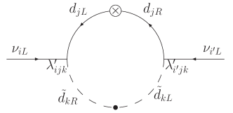
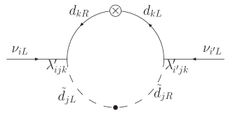
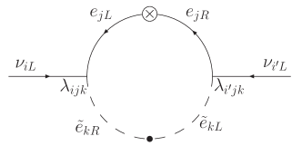
Figure 2: The basic 1–loop diagrams giving rise to the Majorana neutrino mass in the $R$-parity violating MSSM. The transition magnetic moment is obtained by attaching an external photon to the loops.

The introduction of supersymmetry means doubling the number of particles and introducing a lot of new possible interactions among them. SUSY with broken $R$-parity extends the possibility of exotic processes to occur. It is well known, for example, that Majorana neutrinos may acquire masses without the see-saw mechanism, due to one-loop processes in which a neutrino decays into a particle-sparticle pair, which combines into another neutrino of different flavour. The leading contributions to such a process are schematically depicted on Fig. 2. In this paper we consider two possibilities, with a quark and a squark, and with a charged lepton and a slepton inside the loop. Other contributions, like the mixing of neutrinos with neutralinos, are much weaker mg-art15 and are dropped here.

These processes effectively expand the neutrino–neutrino interaction vertex into a loop of virtual charged particles. This means that one may attach an external photon to the loop; the amplitude of such interaction would be proportional to the neutrino magnetic moment. The observation of the electromagnetic interaction of a neutrino will be a strong suggestion in favour of the RpV physics.

The problem of generating neutrino mass matrix from the RpV loops has been extensively discussed in the literature Haug ; Bhatta ; Abada ; rpvneutrinos , and various approaches and approximations have been used by different authors. Our method mg ; mg-art09 ; mg-art15 , which involves the careful generation of the low-energy spectrum of the model seems to be the most complete by now. The calculation of the magnetic moments bases on the knowledge of the neutrino mass matrix, and the latter may be obtained from the experimental values of the mixing angles, under the assumption of certain (normal or inverted) hierarchy of the neutrino masses.

The contribution to the magnetic moments coming from the squark–quark loop reads mg-art09 :

$$\mu_{\nu_{ii^{\prime}}}^{q} = (1-\delta_{ii^{\prime}})\frac{12Q_{d}m_{e}}{16\pi^{2}}\sum_{jkl}\Bigg{\{}\lambda^{\prime}_{ijk}\lambda^{\prime}_{i^{\prime}kl}\sum_{a}V_{ja}V_{la}\frac{w^{q}_{ak}}{m_{d^{a}}}$$ (15)

$$- \lambda^{\prime}_{ijk}\lambda^{\prime}_{i^{\prime}lj}\sum_{a}V_{ka}V_{la}\frac{w^{q}_{aj}}{m_{d^{a}}}\Bigg{\}}\mu_{B},$$

where the loop integral $w$ takes the form

$$w^{q}_{jk}=\frac{\sin 2\theta^{k}}{2}\left(\frac{x_{2}^{jk}\ln x_{2}^{jk}-x_{2}^{jk}+1}{(1-x_{2}^{jk})^{2}}-(x_{2}\to x_{1})\right).$$ (16)

Here $Q_{d}=1/3$ is the $d$-quark charge in units of $e$, and $m_{e}$ denotes the electron mass. $V=V_{\rm CKM}$ is the Cabibbo–Kobayashi–Maskawa quark mixing matrix, as we take into account the fact that quarks may mix inside the loops. $\mu_{B}$ denotes the Bohr magneton. We have defined dimensionless quantities $x_{1}^{jk}\equiv m_{d^{j}}^{2}/m_{\tilde{d}_{1}^{k}}^{2}$ and $x_{2}^{jk}\equiv m_{d^{j}}^{2}/m_{\tilde{d}_{2}^{k}}^{2}$ representing particle to sparticle mass ratios squared.

In the case of the slepton–lepton loop two modifications are in order. Firstly, the mixing of leptons is negligible, secondly, leptons are colorless, so a factor of three drops out from the formula. We end up with:

$$\mu_{\nu_{ii^{\prime}}}^{\ell} = (1-\delta_{ii^{\prime}})\frac{4Q_{e}m_{e}}{16\pi^{2}}$$

$$\times \sum_{jk}\lambda_{ijk}\lambda_{i^{\prime}kj}\left(\frac{w^{\ell}_{jk}}{m_{e^{j}}}-\frac{w^{\ell}_{kj}}{m_{e^{k}}}\right)\mu_{B},$$

where the loop integral is equal to

$$w^{\ell}_{jk}=\frac{\sin 2\phi^{k}}{2}\left(\frac{y_{2}^{jk}\ln y_{2}^{jk}-y_{2}^{jk}+1}{(1-y_{2}^{jk})^{2}}-(y_{2}\to y_{1})\right).$$ (18)

Again, we have defined dimensionless quantities $y_{1}^{jk}\equiv m_{e^{j}}^{2}/m_{\tilde{e}_{1}^{k}}^{2}$ and $y_{2}^{jk}\equiv m_{e^{j}}^{2}/m_{\tilde{e}_{2}^{k}}^{2}$.

As one can see, in order to calculate $\mu_{\nu}$ one needs to know the RpV couplings $\lambda$ and $\lambda^{\prime}$. These are in principle unknown free parameters of the model but fortunately it is possible to get rid of this obstacle by the use of the mass matrices. The latter may be expressed as

$${\cal M}_{ii^{\prime}}^{q} = \frac{3}{16\pi^{2}}\sum_{jkl}\Bigg{\{}\left(\lambda^{\prime}_{ijk}\lambda^{\prime}_{i^{\prime}kl}\sum_{a}V_{ja}V_{la}v^{q}_{ak}m_{d^{a}}\right)$$ (19)

$$+ \left(\lambda^{\prime}_{ijk}\lambda^{\prime}_{i^{\prime}lj}\sum_{a}V_{ka}V_{la}v^{q}_{aj}m_{d^{a}}\right)\Bigg{\}},$$

$${\cal M}_{ii^{\prime}}^{\ell}=\frac{1}{16\pi^{2}}\sum_{jk}\lambda_{ijk}\lambda_{i^{\prime}kj}(v^{\ell}_{jk}m_{e^{j}}+v^{\ell}_{kj}m_{e^{k}}),$$ (20)

with $v^{\ell,q}$ being another loop integrals mg-art09 . Now, we assume that each mechanism (ie. each combination of indices labeling $\lambda$ and $\lambda^{\prime}$) may be analyzed separately. This is a usual approach, which is justified by the assumption that there is no fine-tuning between different processes that contribute to $\cal M$. In this convenient situation only one element from the sums in $\cal M$ is present at a time, thus reducing the expressions to a much simpler form. This allows one to substitute the unknown products $\lambda\lambda$ and $\lambda^{\prime}\lambda^{\prime}$ in Eqs. (15) and (IV) by the respective mass matrix elements. The advantage of such approach is obvious, as one may construct $\cal M$ numerically using experimental data.

Finally one gets for the magnetic moments (for more details see Ref. mg-art09 )

$$\mu_{\nu_{ii^{\prime}}}^{q} \simeq (1-\delta_{ii^{\prime}}){\cal M}^{q}_{ii^{\prime}}f^{q}_{\rm SUSY},$$ (21)

$$\mu_{\nu_{ii^{\prime}}}^{\ell} \simeq (1-\delta_{ii^{\prime}}){\cal M}^{\ell}_{ii^{\prime}}f^{\ell}_{\rm SUSY},$$ (22)

where the functions $f_{\rm SUSY}$ convert the neutrino masses into magnetic moments and depend on the particles masses and V matrix elements. Their explicit form and values for different SUSY input parameters can be found in mg-art09 , but overall these are numbers between roughly $0.5\times 10^{-15}$ and $2.7\times 10^{-18}$. The full transition magnetic moment would consist of both contributions, ie.

$$\mu_{\nu_{ii^{\prime}}}=\mu_{\nu_{ii^{\prime}}}^{\ell}+\mu_{\nu_{ii^{\prime}}}^{q}.$$ (23)

Table 1: Lower and upper bounds on the Majorana neutrino transition magnetic moments in GMSB MSSM, assuming normal (NH) or inverted hierarchy (IH), and two different structures of the messenger sector with the generation index $N=1,4$. The whole allowed parameter space has been considered. Here, sgn$(\mu)=+1$. The unit is the Bohr magneton $\mu_{B}$.

hier.	N	$\mu_{\nu_{e\mu}}$, $\mu_{\nu_{e\tau}}$	$\mu_{\nu_{\mu\tau}}$
NH	1	$(0.38,28.3)\times 10^{-19}$	$(0.28,20.5)\times 10^{-18}$
NH	4	$(0.73,66.1)\times 10^{-20}$	$(0.53,47.9)\times 10^{-19}$
IH	1	$(0.36,26.2)\times 10^{-20}$	$(0.33,24.0)\times 10^{-18}$
IH	4	$(0.68,61.3)\times 10^{-21}$	$(0.62,56.0)\times 10^{-19}$

Table 2: Same as Tab.1 but for sgn$(\mu)=-1$.

hier.	N	$\mu_{\nu_{e\mu}}$, $\mu_{\nu_{e\tau}}$	$\mu_{\nu_{\mu\tau}}$
NH	1	$(0.39,23.8)\times 10^{-19}$	$(0.28,17.3)\times 10^{-18}$
NH	4	$(0.16,6.67)\times 10^{-19}$	$(0.11,4.84)\times 10^{-18}$
IH	1	$(0.36,22.1)\times 10^{-20}$	$(0.33,20.2)\times 10^{-18}$
IH	4	$(0.15,6.19)\times 10^{-20}$	$(0.13,5.65)\times 10^{-18}$

Figure 3: Neutrino magnetic moment $\mu_{\nu_{e\mu}}$ for certain values of the GMSB parameters. Here, sgn$(\mu)=+1$ and normal hierarchy of neutrino masses is assumed.

Figure 4: Same as Fig. 3 but for sgn$(\mu)=-1$.

We have calculated the transition magnetic moments $\mu_{\nu_{e\mu}}$, $\mu_{\nu_{e\tau}}$, and $\mu_{\nu_{\mu\tau}}$ using the following values of the input parameters:

$$3\leq\tan\beta\leq 40,$$ (24)

$$100\hbox{ TeV}\leq\Lambda<M,$$ (25)

$$M=200,500,800,1000\hbox{ TeV},$$ (26)

$$\mathrm{sgn}(\mu)=\pm 1,\quad N=1,4.$$ (27)

The $\Lambda$ parameter was incremented by 1 for $M=200\hbox{ TeV}$, and by 10 for $M=500,800,1000\hbox{ TeV}$. $\tan\beta$ was incremented by 1.

The construction of the neutrino mass matrix ${\cal M}$ is straightforward. We use the standard trigonometric parameterization of ${\cal M}$ and the following values of the mass and mixing parameters nu-osc ; nu-mass : $\Delta m_{12}^{2}=7.1\times 10^{-5}\hbox{ eV}^{2}$, $\Delta m_{23}^{2}=2.1\times 10^{-3}\hbox{ eV}^{2}$, $\sin^{2}(\theta_{12})=0.2857$, $\sin^{2}(\theta_{23})=0.5$, $\sin^{2}(\theta_{13})=0$. As will be seen later, the actual numbers chosen here are not essential. In the matter of fact, one of the most recent analysis suggests the best-fit value of the $\sin^{2}(\theta_{13})$ parameter to be slightly above zero fogli . However, in our case this change plays no role, as the dominant part, which determines the overall order of magnitude of $\mu_{\nu}$, is the $f_{\rm SUSY}$ function. Additionally, we assume that the lightest neutrino mass is zero, and that the CP symmetry is conserved, which eliminates all the phase dependencies. This results for the normal hierarchy (NH) in

$${\cal M}^{\rm NH}=\pmatrix{2.41&2.69&2.69\cr 2.69&25.53&19.51\cr 2.69&19.51&25.53}\hbox{ meV},$$ (28)

and for the inverted hierarchy (IH) in

$${\cal M}^{\rm IH}=\pmatrix{45.27&0.25&0.25\cr 0.25&22.80&22.80\cr 0.25&22.80&22.80}\hbox{ meV}.$$ (29)

Fig. 3 presents values of the $\mu_{\nu_{e\mu}}$ transition magnetic moment for sgn$(\mu)=+1$ and normal hierarchy of the neutrino masses. The non-rectangular shapes come from the constraints on the low-energy spectrum, and the higher the value of $M$ is chosen, the more steep the results are. For example, for $M\sim 1000\hbox{ TeV}$ the difference between lowest and highest values of $\mu_{\nu}$ reaches three orders of magnitude, while for small $M\sim 200\hbox{ TeV}$ $\mu_{\nu}$ is nearly constant. The dependence on $\Lambda$ is monotonic, but changes its character for $\tan\beta$ equals roughly 25. For small $\tan\beta$ $\mu_{\nu}$ is an decreasing function of $\Lambda$, while for high $\tan\beta$ it becomes an increasing function. The steepness of this function, as was stated above, increases with $M$. The general behaviour is that for small $\Lambda$ the dependence on $\tan\beta$ becomes strong, while the values of $\mu_{\nu_{e\mu}}$ converge for higher $\Lambda$ and become nearly insensitive on $\tan\beta$. The difference between $N=1$ and $N=4$ is that for higher $N$ the overall order of magnitude is decreased by one. Also the resulting mass spectrum is different, so that the shapes in Fig. 3 (lower row) are more constrained, than those for $N=1$ (upper row).

A similar plot for sgn$(\mu)=-1$ is presented on Fig. 4. The change in the sign of the $\mu$ parameter results in a completely different behaviour of the magnetic moments as functions of the input parameters. For $N=1$ there are two discontinued regions, which separate roughly at $\Lambda\approx 200\hbox{ TeV}$. The remark about monotonicity and its dependence on $\tan\beta$, which was visible in the previous case, is valid also here, but to much weaker extend, except the narrow region $\Lambda\approx 200\hbox{ TeV}$. Of course, for the case $M=200\hbox{ TeV}$, for which $\Lambda<200\hbox{ TeV}$ (recall that always $\Lambda<M$), this feature isn’t present. So for sgn$(\mu)=-1$ and $N=1$ the $\Lambda$ parameter dominates the change in behaviour of the magnetic moments. When switching to $N=4$, the shapes become nearly smooth surfaces. The dependence on $\tan\beta$ is quite weak, in comparison with the previous cases, while the dependence on $\Lambda$ is a monotonic one with decreasing character. The $M$ parameter shows its impact in the same way as for sgn$(\mu)=+1$, ie. it stretches the shapes along the $\mu_{\nu}$ axis. The gain here is only one order of magnitude, when comparing the cases $M=200\hbox{ TeV}$ and $M=1000\hbox{ TeV}$.

It is worth to notice, that the assumption of inverted hierarchy would not change qualitatively the behaviour of $\mu_{\nu}$, and therefore we do not include separate plots for this case. The only change would be an overall shift of the results along the $\mu_{\nu}$ axis, according to different values of the mass matrix elements for the NH and IH cases.

Also the remaining two transition magnetic moments, $\mu_{\nu_{e\tau}}$ and $\mu_{\nu_{\mu\tau}}$, exhibit very similar behaviour. The $\mu_{\nu_{e\tau}}$ magnetic moment is to a very good approximation equal to $\mu_{\nu_{e\mu}}$, while the $\mu_{\nu_{\mu\tau}}$ will have values shifted up by roughly one order of magnitude (see below).

A summary of the upper and lower limits of the magnetic moments for all considered combinations of the input parameters are presented in Tabs. 1 and 2. In most cases, they span over two-three orders of magnitude. There is also a general trend that $\mu_{\nu_{\mu\tau}}$ has a factor of 10 higher values than $\mu_{\nu_{e\mu}}\approx\mu_{\nu_{e\tau}}$, which comes from the fact that respective mass matrix elements scale in the same way [cf. Eqs. (28) and (29)].

V Conclusions

In the present paper we have used the gauge mediated supersymmetry breaking version of the minimal supersymmetric standard model without $R$-parity to calculate Majorana neutrino transition magnetic moments. In order to reduce the number of free parameters, we have assumed a GUT unification at high energy scale $m_{\rm GUT}\sim 10^{16}\hbox{ GeV}$, and then used the RGE equations to render the values of mass parameters and coupling constants to the low-energy regime.

The magnetic moments are in our approach dependent on the choice of the following parameters: $\Lambda$, $M$, $N$, $\tan\beta$, sgn$(\mu)$, and the phenomenological neutrino mass matrix ${\cal M}$. The latter can be calculated using the mixing parameters extracted from experiments, assuming normal or inverted pattern of neutrino mass hierarchy.

We have discovered that the weakest dependence of $\mu_{\nu}$ comes from the ${\cal M}$ matrix, which enters the formulas (21) as a simple multiplicative factor. The dependence on $\Lambda$, $M$, $N$, and $\tan\beta$ is rather complicated and difficult to describe. It is presented on Figs. 3 and 4. A substantial qualitative change in the behaviour of $\mu_{\nu}$ can be observed when the sign of the $\mu$ parameter is changed. In general, while for sgn$(\mu)=+1$ the small and large values of $\tan\beta$ changed qualitatively the behaviour of $\mu_{\nu}$, such a collapse for sgn$(\mu)=-1$ is driven by the $\Lambda$ parameter.

This all shows, that even if the neutrino magnetic moment would be observed in an experiment, in most cases it will not allow to state definite conclusions about the values of the paramaters in the context of the discussed model. With some luck, it may, however, serve as a clue about the neutrino mass hierarchy, if it happens to place in a region covered by only one range listed in Tabs. 1 and 2.

References

- (1) S. Fukuda et al. (Super-Kamiokande Collaboration), Phys. Rev. Lett. 81, 1562 (1998); Y. Ashie et al. (Super-Kamiokande Collaboration), Phys. Rev. Lett. 93, 101801 (2004); Phys. Rev. D 71, 112005 (2005); T. Araki et al. (KamLAND Collaboration), Phys. Rev. Lett. 94, 081801 (2005); Q.R. Ahmed et al. (SNO Collaboration), Phys. Rev. Lett. 87, 071301 (2001); Phys. Rev. Lett. 89, 011301 (2002); Phys. Rev. Lett. 89, 011302 (2002); B. Aharmin et al. (SNO Collaboration), Phys. Rev. C 72 055502 (2005); M. Apollonio et al. (CHOOZ Collaboration), Phys. Lett. B 466, 415 (1999); Eur. Phys. J. C 27, 331 (2003); G.L. Fogli, et al., Phys. Rev. D 66, 093008 (2002).
- (2) H.E. Haber and G.L. Kane, Phys. Rep. 117, 75 (1985).
- (3) D.I. Kazakov, Beyond the Standard Model (In Search of Supersymmetry), lectures given at the European School on High Energy Physics, Caramulo (2000), and Schwarzwald Workshop, Bad Liebenzell (2000), hep-ph/0012288.
- (4) R. Barbier et al., Phys. Rep. 420, 1 (2005).
- (5) C. Aulakh and R. Mohapatra, Phys. Lett. B 119, 136 (1982); G.G. Ross and J.W.F Valle, Phys. Lett. B 151, 375 (1985); J. Ellis et al., Phys. Lett. B 150, 142 (1985); A. Santamaria and J.W.F. Valle, Phys. Lett. B 195, 423 (1987); Phys. Rev. D 39, 1780 (1989); Phys. Rev. Lett. 60, 397 (1988); A. Masiero and J.W.F. Valle, Phys. Lett. B 251, 273 (1990).
- (6) M.A. Diaz, J.C. Romao, and J.W.F. Valle, Nucl. Phys. B 524, 23 (1998); A. Akeroyd et al., Nucl. Phys. B 529,3 (1998); A.S. Joshipura, M. Nowakowski, Phys. Rev. D 51, 2421 (1995); Phys. Rev. D 51, 5271 (1995).
- (7) M. Nowakowski and A. Pilaftsis, Nucl. Phys. B 461, 19 (1996).
- (8) L.J. Hall and M. Suzuki, Nucl. Phys. B 231, 419 (1984); G.G. Ross and J.W.F. Valle, Phys. Lett. B 151, 375 (1985); R. Barbieri, D.E. Brahm, L.J. Hall, and S.D. Hsu, Phys. Lett. B 238, 86 (1990); J.C. Ramao and J.W.F. Valle, Nucl. Phys. B 381, 87 (1992); H. Dreiner and G.G. Ross, Nucl. Phys. B 410, 188 (1993); D. Comelli et al., Phys. Lett. B 324, 397 (1994); G. Bhattacharyya, D. Choudhury, and K. Sridhar, Phys. Lett. B 355, 193 (1995); G. Bhattacharyya and A. Raychaudhuri, Phys. Lett. B 374, 93 (1996); A.Y. Smirnov, F. Vissani, Phys. Lett. B 380, 317 (1996); L.J. Hall and M. Suzuki, Nucl. Phys. B 231, 419 (1984).
- (9) O. Haug, J.D. Vergados, A. Faessler, and S. Kovalenko, Nucl. Phys. B 565, 38 (2000).
- (10) G. Bhattacharyya, H.V. Klapdor-Kleingrothaus, and H. Päs, Phys. Lett. B 463, 77 (1999).
- (11) A. Abada and M. Losada, Phys. Lett. B 492, 310 (2000); Nucl. Phys. B, 585, 45 (2000).
- (12) S. Davidson and M. Losada, Phys. Rev. D 65 075025 (2002); Y. Grossman and S. Rakshit, Phys. Rev. D 69 093002 (2004).
- (13) M. Góźdź, W.A. Kamiński, and F. Šimkovic, Phys. Rev. D 70, 095005 (2004); Int. J. Mod. Phys. E, 15, 441 (2006); Acta Phys. Polon. B 37, 2203 (2006).
- (14) M. Góźdź, W.A. Kamiński, F. Šimkovic, and A. Faessler, Phys. Rev. D 74 055007 (2006).
- (15) M. Góźdź, W.A. Kamiński, Phys. Rev. D 78, 075021 (2008).
- (16) H.P. Nilles, Phys. Lett. B 115, 193 (1982); A.H. Chamseddine, R. Arnowitt, and P. Nath, Phys. Rev. Lett. 49, 970 (1982); Nucl. Phys. B 227, 121 (1983); R. Barbieri, S. Ferrara, and C.A. Savoy, Phys. Lett. B 119, 343 (1982); E. Cremmer, P. Fayet and L. Girardello, Phys. Lett. B 122, 41 (1983); L. Ibáñez, Phys. Lett. B 118, 73 (1982); H. P. Nilles, M. Srednicki, and D. Wyler, Phys. Lett. B 120, 346 (1983).
- (17) M. Dine and A.E. Nelson, Phys. Rev. D 48, 1277 (1993); M. Dine, A.E. Nelson, and Y. Shirman, Phys. Rev. D 51, 1362 (1995); M. Dine, A.E. Nelson, Y. Nir, and Y. Shirman, Phys. Rev. D 53, 2658 (1996).
- (18) M. Góźdź, W.A. Kamiński, and A. Wodecki, Phys, Rev. C 69, 025501 (2004).
- (19) D.R.T. Jones, Phys. Rev. D 25, 581 (1982).
- (20) S.P. Martin and M.T. Vaughn, Phys. Rev. D 50, 2282 (1994).
- (21) M. Góźdź and W.A. Kamiński, Phys. Rev. D 69, 076005 (2004).
- (22) G. Altarelli and F. Feruglio, New J.Phys. 6, 106 (2004), and references therein.
- (23) G.L. Fogli et al., Phys. Rev. D 78, 033010 (2008).