Electrodynamics of a split-ring Josephson resonator in a microwave line

Abstract

We consider the coupling of an electromagnetic wave to a split-ring Josephson oscillator or radio-frequency SQUID in the hysteretic regime. This device is similar to an atomic system in that it has a number of steady states. We show that one can switch between these with a suitable short external microwave pulse. The steady states can be characterized by their resonant lines which are of the Fano type. Using a static magnetic field, we can shift these spectral lines and lift their degeneracy.

I Introduction

In the past decade artificial materials (metamaterials) have been developed by inserting metal split-rings or rods as metaatoms into dielectric materials. This way negative index materials have been fabricated Veselago:06 , Pendry:04 . These metaatoms spaced periodically enable the medium to have an engineered electromagnetic response. In principle such an artificial atom has many advantages over a real atom. In real materials, the dipole moment of the atom is very small and the interaction with electromagnetic field is small. Therefore to realize significant interactions, large densities are necessary. On the contrary an artificial atom can be constructed with a high dielectric or a high magnetic dipole moment so that it will respond strongly to electromagnetic waves.

Many candidates for artificial atoms have been proposed, most of them with intrinsic nonlinearities. Among them are resonant conductive elements with inserted (nonlinear) diodes Lapin:2003 , split-ring resonators loaded with varactor diodes Katko:2010 , Kerr materials Zharov:2003 or laser amplifiers Gabitov_Kennedy:2010 . Unfortunately many of these systems exhibit large losses. To remedy this problem it has been been suggested to work with superconducting split-ring resonator arrays. An example is the study Chen:Yang:10 using from high-temperature superconducting films. See also the review Anlage:11 for more details.

Among these superconducting meta-materials are the split-ring Josephson resonators subsequently referred to as SRR-JJ where a Josephson junction, a superconducting weak link, is embedded in the slit. In the Josephson community, this device is called an RF SQUID for Radio Frequency Superconducting Quantum Interference Device Barone Likharev .

The device we consider is shown in the left panel of Fig. 1. It is a split ring resonator in which is embedded a Josephson junction. Practically it can be made using a ring like strip of superconducting material where a small region was oxidized to make the junction. The right panel of Fig. 1 shows the electric representation of the device, an inductance $L$ for the strip and the Resistive Shunted Junction (RSJ) model for the Josephson junction (JJ). The latter represents the junction as a resistor $R$, a capacity $C$ and the nonlinear element in parallel. This last element is the sine coupling $I_{c}\sin(\Phi/\Phi_{0})$ where $\Phi$ is the magnetic flux and $\Phi_{0}$ is the reduced flux quantum $\Phi_{0}=\hbar/(2e)$.

The use of these devices in metamaterials was advocated by Lazarides Lazarides:06 lt07 and by the authors Maim:Gabi:10 . The electrodynamics of such metamaterials where split-rings are coupled inductively was investigated in Lazarides:06 ; lt07 . It leads to a 2D discrete sine-Gordon equation. For weak external radio-frequency forcing and small densities, this dilute gas of artificial atoms demonstrates a nonlinear magnetic response Maim:Gabi:07 .

Such arrays of SRR-JJ are difficult to analyze because the coupling between the artificial atoms is partly inductive, partly capacitive. Another point is that the field couples to the phase of the Josephson junctions so that the system should have two components. For these reasons, in this article we study the dilute system where each SRR-JJ can be considered as isolated although coupled to an electromagnetic wave. We consider the so-called hysteretic regime where the system has controlled metastable states and show that one can switch from the ground state to one of these excited states by applying a suitable flux pulse. Then we can detect these states by examining the reflection coefficient of an electromagnetic wave incident on the device, this is a kind of spectroscopy. More precisely, the resonance observed are asymetric, of the Fano type. This is interesting because it is observed for many plasmonic systemskivshar_fano .

The article is organized as such. In section 2 we present the basic equations of the model and analyze it’s steady states. In section 3 we show how to switch from one state to another by applying a suitable flux pulse. Section IV discusses the scattering of an electromagnetic wave by a SRR-JJ and this leads to a spectroscopy of the steady states.

II The model

We consider here that the SRR-JJ is subject to irradiation by a microwave field. The equations describing the system light-ring are the generalized pendulum equation for the flux and the Maxwell equation for the electromagnetic field. The Maxwell equations can be written as

$$\nabla\times\mathbf{E} =-\mathbf{B}_{,t},\qquad\nabla\cdot\mathbf{D}=0,$$

$$\nabla\times\mathbf{B} =\mathbf{E}_{,t},\qquad\nabla\cdot\mathbf{B}=0.$$

where ${\bf E}$ and ${\bf H}$ are respectively the electric field and the magnetic field, and the subscritpts indicate the partial derivative. The fields $\mathbf{B},{\bf H}$ and $\mathbf{E},\mathbf{D}$ are related by

$$\mathbf{B}=\mu_{0}\mathbf{H}+\mathbf{M},\qquad\mathbf{D}=\varepsilon_{0}\mathbf{E}+\mathbf{P},$$

where $\mathbf{M}$ and $\mathbf{P}$ are respectively the magnetization and polarisation of the medium. In the dispersionless limit we can write $\mathbf{D}=\varepsilon_{0}\varepsilon\mathbf{E}$ . The magnetization $\mathbf{M}$ is located in the thin plane layer that is embedded into a dielectric surrounding with permittivity $\varepsilon$ at a point $z=0$. The magnetization can then be represented as

$$\mathbf{M}(t,\mathbf{r})=\mathbf{m}(t)n_{r}l\delta(z),$$

where $l$ is the film thickness, $n_{r}$ is the density of SRR-JJ and $\mathbf{m}(t)$ is the magnetic moment of the ring Maim:Gabi:10 .

We assume that the plane electromagnetic wave propagates along the z-axis and is polarized so that $\mathbf{H}$ is parallel to the y axis, the normal to the plane of the SRR-JJ and $\mathbf{E}$ is parallel to the x axis (see Fig. 1). Since all the magnetic moments of the SRR-JJ in the layer are parallel, the magnetization is parallel to $\mathbf{H}$. In this case the Maxwell equations take the form

$$E_{,z}=-(\mu_{0}H_{,t}+M_{,t}),\qquad H_{,z}=-\varepsilon_{0}\varepsilon E_{,t}.$$

They imply the wave equation

$$H_{,zz}-\mu_{0}\varepsilon_{0}\varepsilon H_{,tt}=\varepsilon_{0}M_{,tt}$$ (1)

Ohm’s law applied to the ring gives

$$\mathcal{E}=U_{L}+U_{C},$$

where $\mathcal{E}$ is the electromotive force induced by the magnetic field of the electromagnetic pulse incident on the ring.

$$\mathcal{E}=-\frac{\partial\Phi}{\partial t}\approx-SH_{,t}(0,t),$$

and where $S$ is the surface enclosed by the ring. We neglect the resistance of this loop which we assume to be made of superconductive material. Following Josephson’s second relation, the voltage across the junction is

$$U_{C}=\frac{\hbar}{2e}\frac{\partial\varphi}{\partial t}=\Phi_{0}\frac{\partial\varphi}{\partial t},$$

where $\varphi$ is the phase of the junction. The inductance $L$ due to the loop of the SRR results in the voltage

$$U_{L}=L\frac{\partial I}{\partial t}$$

where $I$ is the current in the loop. Taking into account Ohm’s law together with these definitions we obtain

$$\Phi+\Phi_{0}\varphi+LI=0,$$

or

$$I=-L^{-1}(\Phi+\Phi_{0}\varphi).$$ (2)

The Resistive Shunted Junction model for the Josephson junction together with Kirchoff’s law for the current imply

$$I=I_{C}+I_{J}+I_{R}=C\frac{\partial U_{C}}{\partial t}+I_{c}\sin\varphi+I_{R}$$

$$=C\Phi_{0}\frac{\partial^{2}\varphi}{\partial t^{2}}+I_{c}\sin\varphi+{\Phi_{0}\over R}\frac{\partial\varphi}{\partial t}$$

Thus the variable $\varphi$ evolves according to

$$C\Phi_{0}\frac{\partial^{2}\varphi}{\partial t^{2}}+{\Phi_{0}\over R}\frac{\partial\varphi}{\partial t}+I_{c}\sin\varphi=-L^{-1}(\Phi+\Phi_{0}\varphi).$$

In this equation the flux $\Phi$ has two components, the incident magnetic flux and the flux induced by the current in the loop of the SRR-JJ. That is

$$\Phi=SH_{in}(t)-\frac{S}{2}\sqrt{\frac{\varepsilon_{0}}{\varepsilon\mu_{0}}}\frac{\partial M}{\partial t}.$$

Since $M=n_{r}lSI(t)$ we have

$$M=-n_{r}lSL^{-1}(\Phi+\Phi_{0}\varphi).$$

The wave equation (1) can be rewritten as

$$H_{,zz}-\mu_{0}\varepsilon_{0}\varepsilon H_{,tt}=\varepsilon_{0}\tilde{m}_{,tt}\delta(z)$$

where the one ring magnetization $\tilde{m}$ can be defined as

$$\tilde{m}(t)=n_{r}lSI(t).$$

Taking into account the definition of the current (2) one can write

$$\tilde{m}(t)=-n_{r}lSL^{-1}(\Phi+\Phi_{0}\varphi)=-n_{r}lSL^{-1}(SH+\Phi_{0}\varphi).$$

The phase variable $\varphi$ is governed by the equation

$$\frac{\partial^{2}\varphi}{\partial t^{2}}+{1\over RC}\frac{\partial\varphi}{\partial t}+\frac{I_{c}}{C\Phi_{0}}\sin\varphi=-{1\over LC}\frac{SH(0,t)}{\Phi_{0}}.$$

The natural units of time, flux and space are given by

$$\omega_{T}=1/\sqrt{LC},~{}~{}\Phi_{0},~{}~{}z_{0}={c\over\omega_{T}\sqrt{\varepsilon}},$$

where $\omega_{T}$ is the Thompson frequency and $z_{0}$ is the inverse of the Thompson wave number. Hence, we can introduce the new dimensionless variables

$$h=SH/\Phi_{0},\qquad\tau=\omega_{T}t,\qquad\zeta=z/z_{0}.$$

In terms of these variables the final equations are

$$h_{,\zeta\zeta}-h_{,\tau\tau}=-\kappa(h+\varphi)_{,\tau\tau}\delta(\zeta),$$ (3)

$$\varphi_{,\tau\tau}+\alpha\varphi_{,\tau}+\varphi+\beta\sin\varphi=-h,$$ (4)

where the parameters $\alpha,~{}~{}\beta$ and $\kappa$ are

$$\alpha={1\over R}\sqrt{L\over C},~{}~{}\beta={LI_{c}\over\Phi_{0}},~{}~{}\kappa=\frac{n_{r}lS\varepsilon_{0}\omega_{T}}{L\sqrt{\varepsilon}}.$$

Figure 1: The left panel shows a schematic view of the electromagnetic wave incident on the split ring Josephson junction resonator in the $(y,z)$ plane. The right panel shows the equivalent circuit of the split-ring using the Resistively Shunted Junction model for the Josephson junction.

The system of equations (3,4) is our principal model and we will investigate it in detail throughout the article.

Let us briefly recall the main properties of the SRR-JJ equation (4). It can be written as the 1st order system

$$\varphi_{,\tau}=\psi,$$ (5)

$$\psi_{,\tau}=-\alpha\psi-\beta\sin(\varphi)-\varphi+h,$$ (6)

whose fixed points are $(0,0)$ and $(\varphi^{*},0)$ where

$$-\beta\sin(\varphi^{*})-\varphi^{*}+h=0.$$ (7)

A plot of the above relation indicates that for $\beta<4.34$, the equation has no solution so that there is only the $(0,0)$ fixed point. For large $\beta$, the fixed points can be approximated using an asymptotic expansion

$$\varphi^{*}=\varphi^{(0)}+{1\over\beta}\varphi^{(1)}+{1\over\beta^{2}}\varphi^{(2)}+\dots$$

We get the approximation of the fixed points as

$$\varphi^{*}=n\pi+{1\over\beta}(-1)^{n}(h-n\pi)+\dots,$$ (8)

where $n$ is an integer.

In the absence of damping $\alpha=0$ and forcing $h=0$, the system is Hamiltonian with

$${\cal H}(\varphi,\varphi_{,\tau})={1\over 2}\varphi_{,\tau}^{2}+\beta(1-\cos\varphi)+{1\over 2}\varphi^{2}\equiv{1\over 2}\varphi_{,\tau}^{2}+U(\varphi).$$ (9)

The stable fixed points correspond to the minima of the potential $U(\varphi)$ and the even values of the integer $n$. Fig. 2 shows a plot of the potential $U(\varphi)$ for $\beta=1,9.76$ and $100$. For $\beta=1$ shown as a continuous curve (red online) there is only one fixed point $\varphi=0$. For $\beta=9.76$ shown in dashed line (green online) there are three minima corresponding to stable fixed points, $\varphi=0,\pm\phi^{*}$ where $\varphi^{*}\approx 2\pi$. For $\beta=100$ there are many stable fixed points.

For this one degree of freedom Hamiltonian, the orbits are the contour levels of the Hamiltonian. An important orbit is the separatrix connecting the two unstable fixed points $\varphi=\varphi^{*}\approx\pi$. It is given by $\mathcal{H}=\mathcal{H}(\varphi^{*},0)$. Fig. 3 shows the phase portrait for $\beta=9.76$. For this value there are only five fixed points. Notice the closed orbits around the fixed points, the closed orbits surrounding the three stable fixed points.

Figure 2: Potential energy $U(\varphi)=\beta(1-\cos\varphi)+{1\over 2}\varphi^{2}$ with three different values of $\beta$, $\beta=1,9.76$ and $100$.

Figure 3: Phase portrait $(\varphi,\varphi_{\tau})$ of the Hamiltonian system (9) ($\alpha=0$) for $\beta=9.76$ and $\mathcal{H}=0$. The contour levels presented are 0.1, 1, 5, 17., 25.0360499136927 (separatrix) , 30.,40. and 50.

Another point is that the incident flux can be used to modify the energy levels of the system. Assuming the incident flux to be constant we can add a term to the potential and obtain the generalized potential

$$U(\varphi)=\beta(1-\cos\varphi)+{1\over 2}\varphi^{2}-h\varphi,$$ (10)

where $h$ is the normalized incident flux, assumed constant. This expression is plotted in Fig. 4 for $\beta=15$ and $h=0,1.8\pi$ and $4.5\pi$. The minima are symmetric for $h=0$ and they are shifted to the left and the corresponding value of the potential is decreased. By applying a sufficiently large continuous field one can then shift the system from one state to the other. Notice that for the large field $h=4.5\pi$, there is a fourth minimum, around $7\pi$.

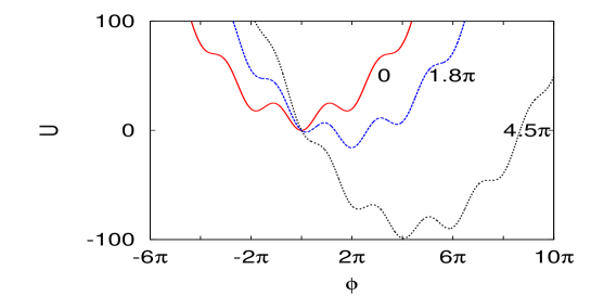
Figure 4: Potential energy $U(\varphi)=\beta(1-\cos\varphi)+{1\over 2}\varphi^{2}-h\varphi$ for three different values of the static incident flux $h=0,1.8\pi$ and $4.5\pi$.

To summarize, the SRR-JJ has energy states $U(\varphi)$ near $2n\pi$. The number of these states is controlled by the parameter $\beta$ i.e. the ratio of the flux to the flux quantum and the magnetic field $h$. In the next section, we will select the incident flux $h$ to move the system from one equilibrium to another.

III Switching between equilibrium states

We consider now that the state of the system can be shifted from one fixed point to another via an incident flux. For a short lived perturbation, the system then relaxes freely to a minimum of energy. The influence of the damping is essential , it should be present to allow the relaxation but small to preserve the picture of the potential. To examine how an incident flux will shift the system from one equilibrium position to another it is useful to analyze the work equation. To obtain it, we multiply (4) by $\varphi_{,\tau}$ and integrate over time. We get the difference in energy

$$E(\tau_{2})-E(\tau_{1})\equiv\left[{1\over 2}\varphi_{,\tau}{}^{2}+\beta(1-\cos\varphi)+{1\over 2}\varphi^{2}\right]_{\tau_{1}}^{\tau_{2}}=$$

$$=\int_{\tau_{1}}^{\tau_{2}}d\tau h\varphi_{\tau}-\alpha\int_{\tau_{1}}^{\tau_{2}}d\tau\varphi_{\tau}^{2}.$$ (11)

The first term on the right hand side is the forcing while the second one is the damping term. When a square pulse is applied to the system, such that

$$h(\tau)=a,~{}{\rm for}~{}\tau_{1}<\tau<\tau_{2},~{}~{}~{}0~{}~{}{\rm elsewhere}$$

the first integral is $a[\varphi(\tau_{2})-\varphi(\tau_{1})]$. If the system is started at $(0,0)$ in phase space so that the $E(\tau_{1})=0$ and $\varphi(\tau_{1})=0$, we have

$$E(\tau_{2})=a\varphi(\tau_{2})-\alpha\int_{\tau_{1}}^{\tau_{2}}d\tau\varphi_{\tau}^{2},$$

so that $\varphi(\tau_{2})$ determines how much energy is fed into the system. When the pulse is long $\tau_{2}>>\tau_{1}$ $\varphi(\tau)$ will relax and oscillate so that there are values of $\tau_{2}$ such that $\varphi(\tau_{2})~{}0$. In that case no energy gets fed into the system. A sure way to avoid this is to take a narrow pulse.

The natural frequency of the oscillator around the $(0,0)$ fixed point is

$$\omega_{0}=\sqrt{\beta+1},$$ (12)

which for $\beta=9.76$ gives $\omega_{0}\approx 3.28$ and a period $T_{0}=2\pi/\omega_{0}\approx 1.91$. To simplify matters we now consider a pulse of duration much smaller than $T_{0}$. This is experimentally feasible. For the present analysis the pulse duration is very small so that it can be approximated by the Dirac delta function $h(\tau)=a\delta(\tau)$, where $a$ is a parameter. Let us analyze briefly the solution. The equation (4) becomes

$$\varphi_{\tau\tau}+(\alpha+\delta)\varphi_{\tau}+\beta\sin(\varphi)+\varphi=a\delta(\tau).$$ (13)

Integrating the equation on a small interval of size $\epsilon$ around 0, we get

$$[\varphi_{\tau}]_{-\epsilon}^{\epsilon}+\alpha[\varphi]_{-\epsilon}^{\epsilon}+\int_{-\epsilon}^{\epsilon}d\tau(\beta\sin\varphi+\varphi)=a.$$ (14)

We now take the limit $\epsilon\to 0$. We will assume continuity of the phase so that $[\varphi]_{-\epsilon}^{\epsilon}\to 0$. The third term being the integral of a continuous function tends to 0 when the bounds tend to 0. Assuming $\varphi_{\tau}(0_{-})=0$ we get $\varphi_{\tau}(0_{+})=a$ so that such a short incident pulse will just give momentum to the system. With these initial conditions we solve equation (4) numerically using a Runge-Kutta algorithm with step correction of order 4 and 5.

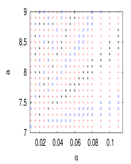
Figure 5: Parameter plane $(\alpha,a)$ showing the different final states reached by the system, the left focus $*$ (blue online), the center focus $+$ (red online) and the right focus $\times$ (green online). The parameter $\beta=9.76$.

We will now explore systematically the plane $(\alpha,a)$ characteristic of the incident pulse. The plot in the $(\alpha,a)$ parameter plane shown in Fig. 5 shows the final states, $O$ the central focus ($+$), $R$ the right focus ($\times$) and $L$ the left focus $*$ reached by the system. Notice how these are organized in ”tongues” following the sequence $O~{}R~{}O~{}L~{}O~{}R~{}O~{}L\dots$ as one sweeps the plane counterclock-wise starting from the horizontal axis. This simple geometrical picture can be understood by examining Fig. 3. In the case of small damping, the separatrices around the fixed points are not affected very much. Their perimeter is proportional to the probability of reaching one fixed point or another. The system is moving clock-wise along the orbits. Assume the system reaches the central point $O$ for a given set of parameters. If the damping is increased, the orbit might not reach $O$ but will settle in $L$. Similarly if more kinetic energy is given to the oscillator, it might reach $R$ instead of $O$.

Another important point is that the impulse given to the resonator must be very short so that it relaxes following a free dynamics. The typical frequencies of these devices are about 500 GHz so the impulse must be around 5 Thz.

Now that we have seen how to prepare the system in a given state, it is important to check if this state is really reached. For that one can use a small signal to analyze the state by reflection or transmission. This is the object of the next section.

IV Microwave spectroscopy of the SRR-JJ

We assume that the ring is submitted to a fixed magnetic field $h_{s}$ and that it is in a local minimum $\varphi_{s}$ of the potential. Then we send in a small electromagnetic pulse $\delta H$ and examine the response $\delta\varphi$ of the ring using the scattering theory. The linearized equations for $\delta h,~{}\delta\varphi$ read

$$\delta h_{\zeta\zeta}-\delta h_{\tau\tau}=-\gamma\left(-\delta\Phi_{\tau\tau}+\delta h_{tt}\right)\delta(\zeta),$$

(15)

$$\delta\Phi_{\tau\tau}+\alpha\delta\Phi_{\tau}+\beta\cos(\varphi_{s})\delta\Phi+\delta\Phi=\delta h.$$

We now assume periodic solutions

$$\delta h=h_{a}e^{i\omega\tau},~{}\delta\varphi=\varphi_{a}e^{i\omega\tau},$$ (16)

and obtain the reduced system

$$h_{a,\zeta\zeta}+\omega^{2}h_{a}=\gamma\omega^{2}\left(-\varphi_{a}+h_{a}\right)\delta(\zeta),$$

(17)

$$\left[-\omega^{2}+i\alpha\omega+1+\beta\cos(\varphi_{s})\right]\varphi_{a}=h_{a}.$$

In the scattering we assume the electromagnetic wave to be incident from the left of the film located at $\zeta=0$. We then have

$$h_{a}=e^{-i\omega\zeta}+\mathcal{R}e^{i\omega\zeta}~{},\zeta<0~{};~{}~{}~{}~{}h_{a}=\mathcal{T}e^{-i\omega\zeta},\zeta>0~{}~{},$$ (18)

where $\mathcal{R}$ is the amplitude of the reflected wave and $\mathcal{T}$ the amplitude of the transmitted wave. We have the following interface conditions at $\zeta=0$

$$h_{a}(0^{-})=h_{a}(0^{+}),~{}~{}[h_{a,\zeta}]_{0^{-}}^{0^{+}}=\omega^{2}\gamma\left(-\varphi_{a}(0)+h_{a}(0)\right).$$ (19)

They imply two equations for $\mathcal{R}$ and $\mathcal{T}$ from which we obtain the transmission coefficient

$$\mathcal{T}={2(-\omega^{2}+1+\beta\cos\varphi_{s}+i\omega\alpha)\over D},$$ (20)

the reflection coefficient

$$\mathcal{R}={-\alpha\gamma\omega^{2}+i\gamma\omega(\beta\cos\varphi_{s}-\omega^{2})\over D},$$ (21)

and where the denominator is

$$D=2(-\omega^{2}+1+\beta\cos\varphi_{s})+\alpha\gamma\omega^{2}+i[2\alpha\omega-\gamma\omega(\beta\cos\varphi_{s}-\omega^{2})].$$ (22)

The square of the modulus of $R$ is

$$|\mathcal{R}|^{2}={\alpha^{2}\gamma^{2}\omega^{4}+\gamma^{2}\omega^{2}(\beta\cos\varphi_{s}-\omega^{2})^{2}\over|D|^{2}}.$$ (23)

As seen in section 3, the split-ring oscillator has a finite number of equilibria $\varphi_{s}$ depending on the parameter $\beta$. We will assume that $\alpha=0$ throughout the section. This damping does not change the width of the resonances, it only affects the bounds of $|R|$. For $\alpha=0,~{}0<|R|<1$ while for $\alpha>0,~{}\alpha<|R|<1-\alpha$. When $\alpha=0$ $|\mathcal{R}|^{2}$ is an even function of $\omega$, therefore we will only consider $\omega>0$.

As a first example we consider $h=0$ and $\beta=9.76$ corresponding to the potential plotted in Fig. 2.

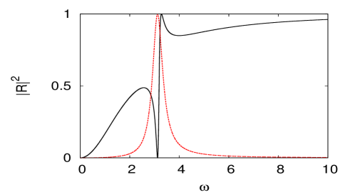
Figure 6: Square of the modulus of the reflection coefficient $|R|^{2}$ as a function of the frequency $\omega$ for $\beta=9.76,~{}h=0,~{}\varphi_{s}=0$ for a large coupling $\gamma=1$. The dashed line (red online) presents the reflection coefficient $|R|^{2}$ for a polarized dielectric film for comparison.

The reflection coefficient is plotted in Fig. 6 for $\gamma=1$ and $\varphi_{s}=0$. Notice how the resonance is asymetric around a minimum $\omega_{s}$. The system is passing for low frequencies only. This line shape is a typical Fano resonance nm11 due to the nonlocal coupling associated to the $\varphi_{\tau\tau}$ term in the right hand side of the wave equation (3). To see this, we have reported in Fig. 6 the reflection coeffcient for a simple polarized dielectric film ckm06 . This simpler system is passing for all frequencies except for a narrow band around the resonant frequency $\omega_{s}$. The expression for the resonant frequencies $\omega_{s}$ can be obtained by considering the minima of $|\mathcal{R}|^{2}$. These correspond to the second term in the numerator of (23) being zero. We get

$$\omega_{s}=\sqrt{\beta\cos\varphi_{s}}.$$ (24)

Let us now examine the influence of the different parameters on the reflection coefficient. Fig. 7 shows the reflection coefficient $|R|^{2}$ for the two steady states $\varphi_{s}$ and $\gamma=1$ (left panel) and $\gamma=0.2$ (right panel).

Figure 7: Square of the modulus of the reflection coefficient $|R|^{2}$ as a function of the frequency $\omega$ for $\beta=9.76$ and $H=0$ for a large coupling $\gamma=1$ (left panel) and a small coupling $\gamma=0.2$ (right panel).

For the large coupling the resonance is sharp although for large $\omega$ we recover $|R|=1$. The value of the steady state $\varphi_{s}$ also influences $|R|$. In Fig. 7, the continuous curve corresponds to $\varphi_{s}=0$ and the dashed line corresponds to $\varphi_{s}=\pm 5.66$, the two additional local minima. The two curves are very close and the reflection coefficient does not indicate if we are in the left or right minimum. Notice also that the system only passes low frequencies for $\gamma=1$. On the contrary for $\gamma=0.2$ it is globally passing for all frequencies except for a narrow band around $\omega_{s}$. These plots would enable to extract the coupling parameter from a SRR-JJ.

As a second example we consider $\beta=9.76$ and $h=1.8\pi$ corresponding to the potential plotted in Fig. 4. There are three minima given in the table I. The reflection coefficient $|R|^{2}$ is plotted in Fig. 8. Now it is possible to distinguish the ”left” minimum 1 from the ”right” minimum 3 because the non zero magnetic field $h$ has lifted the degeneracy.

${\rm index}$	1	2	3
$\varphi_{s}$	0.550	6.224	11.875
$\omega_{s}$	2.884	3.121	2.742

Table 1: Spectroscopy data $(\omega_{s},\varphi_{s})$ for a split-ring oscillator with three steady states. The parameters are $\beta=9.76,~{}~{}h=1.8\pi,~{}\gamma=1,~{}\alpha=0$.

Figure 8: Square of the modulus of the reflection coefficient $|R|^{2}$ as a function of the frequency $\omega$ for the three different equilibria indicated in Table I. The parameters are $\beta=9.76,~{}~{}h=1.8\pi,~{}~{}\gamma=1$ and $\alpha=0$.

Finally we consider $h=0$ and $\beta=30$ for which the potential $U(\phi)$ has five minima indicated in the table II. The square of the modulus of the reflection coefficient (23) is plotted in Fig. 9 for the five different equilibria. In the example shown, the spectroscopy data $(\omega_{s},\varphi_{s})$ is given in table II. Again there is no possibility to distinguish whether the system is in the left or the right minimum.

${\rm index}$	1	2	3	4	5
$\varphi_{s}$	0	6.08	12.15	18.2	24.18
$\omega_{s}$	5.477	5.420	5.238	4.888	4.169

Table 2: Spectroscopy data $(\omega_{s},\varphi_{s})$ for a split-ring oscillator with five steady states. The parameters are $\beta=30,~{}\gamma=1,~{}\alpha=0.01$.

Figure 9: Square of the modulus of the reflection coefficient $|R|^{2}$ as a function of the frequency $\omega$ for the five different equilibria indicated in Table II. The index of the minima is indicated in the plot. The parameters are $\beta=30,~{}~{}\gamma=1$ and $\alpha=0.01$.

V Conclusion

We considered the interaction of an electromagnetic wave with a split-ring Josephson resonator. For appropriately chosen parameters, the resonator has excited states whose number can be controlled by carefully tuning the inductance and capacity of the ring. The existence of these excited states makes this system similar to an artificial atom with discrete energy levels. Other artificial atoms containing nonlinear elements like a diode Lapin:2003 , a Kerr material Zharov:2003 or a laser amplifier Gabitov_Kennedy:2010 would not give these discrete levels. In addition, since the oscillator is operating in the superconducting regime the losses are very small as opposed to the current metamaterials.

First we assumed that there are just two excited states and showed how an incident magnetic flux can shift the system from the ground state to one of these excited states. By sending a microwave field on the resonator we can perform a spectroscopy of it and characterize in which state it is. Using a scattering theory formalism we computed the reflection and transmission coefficients for the wave. These have a specific minimum that we can compute analytically. Another interesting feature is the form of the resonance which is Fano like and very different from the one obtained for a ferroelectric thin film ckm06 . Note that the right and left minima are undistinguishable with this measurement and that a static magnetic field will lift this degeneracy. We hope this analysis will be useful to experimentalists studying split ring Josephson resonators.

Acknowledgements
The authors thank Matteo Cirillo, Alexei Ustinov and Alexey Yulin for very helpful discussions. JGC and AM thank the University of Arizona for its support. AIM is grateful to the Laboratoire de Mathématiques, INSA de Rouen for hospitality and support. The computations were done at the Centre de Ressources Informatiques de Haute-Normandie. This research was supported by RFBR grants No. 09-02-00701-a.

References

- (1) V. Veselago, L. Braginsky, V. Shklover, Ch. Hafner, Negative Refractive Index Materials J. Computational and Theoretical Nanoscience. 3, 1-30 (2006)
- (2) J.B. Pendry, Negative refraction, Contemporary Physics. 45, 191-202 (2004)
- (3) M. Lapine, M. Gorkunov, and K. H. Ringhofer Nonlinearity of a metamaterial arising from diode insertions into resonant conductive elements, Phys.Rev. B67, 065601(R) (2003)
- (4) A.R. Katko, Shi Gu, J.P. Barrett, Bogdan-Ioan Popa, G. Shvets, and S.A. Cummer, Phase Conjugation and Negative Refraction using Nonlinear Active Metamaterials Phys.Rev.Lett. 105, 123905 (2010).
- (5) A.A. Zharov, I.V. Shadrivov, and Yu. S. Kivshar, Nonlinear Properties of Left-Handed Metamaterials, Phys.Rev.Lett. 91, 037401 (2003)
- (6) I.R. Gabitov, B. Kennedy, A.I. Maimistov, Coherent Amplification of Optical Pulses in Metamaterials IEEE Journal of Selected Topics in Quantum Electronics 16, 401 - 409 (2010).
- (7) Hou-Tong Chen, Hao Yang, Ranjan Singh, John F. O’Hara, Abul K. Azad, Stuart A. Trugman, Q. X. Jia, and Antoinette J. Taylor, Tuning the Resonance in High-Temperature Superconducting Terahertz Metamaterials Phys.Rev.Lett. 105, 247402 (2010).
- (8) S. M. Anlage, The physics and applications of superconducting metamaterials J. Opt. 13, 024001 (2011).
- (9) A. Barone and G. Paterno, Physics and Applications of the Josephson effect, J. Wiley, (1982).
- (10) K. Likharev, Dynamics of Josephson junctions and circuits, Gordon and Breach, (1986).
- (11) N. Lazarides, M. Eleftheriou, and G. P. Tsironis, Discrete Breathers in Nonlinear Magnetic Metamaterials, Phys.Rev.Lett. 97, 157406 (2006)
- (12) N. Lazarides and G. P. Tsironis, rf superconducting quantum interference device metamaterials, Appl. Phys. Lett. 90, 163501, (2007).
- (13) A.I. Maimistov, I. Gabitov, Nonlinear response of a thin metamaterial film con-taining Josephson junctions, Opt.Commun. 283, 1633-1639 (2010).
- (14) A.I. Maimistov, I.R. Gabitov, Nonlinear optical effects in artificial materials, Eur. Phys. J. Special Topics. 147, 265-286 (2007)
- (15) A. E. Miroshnichenko, S. Flach and Y. S. Kivshar, Fano resonances in nanoscale structures, Rev. Mod. Phys., 82, 2257 - 2298, (2010).
- (16) U. Naether and M. I Molina, Phys.Rev. A 84, 043808, (2011).
- (17) J.-G. Caputo, E. V. Kazantseva, A.I. Maimistov, Phys.Rev. B 75, 014113, (2007).