Searching for super-WIMPs in leptonic heavy meson decays

Abstract

We study constraints on the models of bosonic super-weakly interacting particle (super-WIMP) dark matter (DM) with DM masses $m_{X}\sim\mathcal{O}(1-100)$ keV from leptonic decays $M\rightarrow\ell\bar{\nu}_{\ell}+X$, where $M=B^{\pm},D^{\pm},D_{s}^{\pm}$ is a heavy meson state. We focus on two cases where $X$ denotes either a light pseudoscalar (axion-like), or a light vector state that couples to the standard model (SM) through kinetic mixing. We note that for a small DM mass these decays are separately sensitive to DM couplings to quarks, but not its mass.

I Introduction

There is evidence that the amount of dark matter (DM) in the Universe by far dominates that of the luminous matter. It comes from a variety of cosmological sources such as the rotation curves of galaxies DMgalaxies , gravitational lensing DMlensing , features of CMB Komatsu:2010fb and large scale structures Allen:2002eu . While the presence of DM is firmly established, its basic properties are still subject of a debate. If dark matter is comprised of some fundamental particle, experimentally-measured properties, such as its relic abundance or production cross-sections can be predicted. Experimental measurements of the abundance $\Omega_{DM}h^{2}\sim 0.12$ by WMAP collaboration WMAP can be used to place constraints on the masses and interaction strengths of those DM particles. Indeed, the relation

$$\Omega_{DM}h^{2}\sim\langle\sigma_{ann}v_{rel}\rangle^{-1}\propto\frac{M^{2}}{g^{4}},$$ (1)

with $M$ and $g$ being the mass and the interaction strength associated with DM annihilation, implies that, for a weakly-interacting massive particle (WIMP) of DM, the mass scale should be set around the electroweak scale. Yet, difficulties in understanding of small-scale gravitational clustering in numerical simulations with WIMPs may lead to preference being given to much lighter DM particles. Particularly there has been interest in studying models of light dark matter particle with masses of the keV range Pospelov:2008jk ; Pospelov:2007mp . According to Eq. (1), the light mass of dark matter particle then implies a superweak interaction between the dark matter and standard model (SM) sector SWIMP:1 . Several models with light $\cal{O}$(keV-MeV) DM particles, or super-WIMPs, have been proposed Pospelov:2008jk ; Pospelov:2007mp .

One of the main features of the super-WIMP models is that DM particles do not need to be stable against decays to even lighter SM particles Pospelov:2008jk . This implies that one does not need to impose an ad-hoc $Z_{2}$ symmetry when constructing an effective Lagrangian for DM interactions with the standard model fields, so DM particles can be emitted and absorbed by SM particles. Due to their extremely small couplings to the SM particles, experimental searches for super-WIMPs must be performed at experiments where large statistics is available. In addition, the experiments must be able to resolve signals with missing energy Batell:2009yf . Super-B factories fit this bill perfectly.

In this paper we focus on bosonic super-WIMP models Pospelov:2008jk ; Pospelov:2007mp for dark matter candidates and attempt to constrain their couplings with the standard model through examining leptonic meson decays. The idea is quite straightforward. In the standard model the leptonic decay width of, say, a $B$-meson, i.e. the process $B\rightarrow\ell\bar{\nu}$, is helicity-suppressed by $(m_{\ell}/m_{B})^{2}$ due to the left-handed nature of weak interactions Rosner:2010ak ,

$$\Gamma(B\rightarrow\ell\bar{\nu})=\frac{G_{F}^{2}}{8\pi}|V_{ub}|^{2}f_{B}^{2}m_{B}^{3}\frac{m_{\ell}^{2}}{m_{B}^{2}}\biggl{(}1-\frac{m_{\ell}^{2}}{m_{B}^{2}}\biggr{)}^{2}.$$ (2)

Similar formulas are available for charmed meson $D^{+}$ and $D_{s}$ decays with obvious substitution of parameters. The only non-perturbative parameter affecting Eq. (2), the heavy meson decay constant $f_{B}$, can be reliably estimated on the lattice Davies:2010ip , so the branching ratio for this process can be predicted quite reliably.

The helicity suppression arises from the necessary helicity flip on the outgoing lepton due to angular momentum conservation as initial state meson is spinless. The suppression can be overcome by introducing a third particle to the final state that contributes to total angular momentum Burdman:1994ip (see Fig. 1).

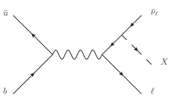
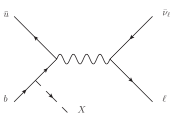
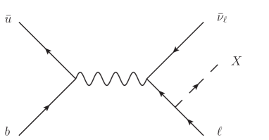
Figure 1: Diagrams for the super-WIMP emission in $B\to\ell\bar{\nu}_{\ell}X$. Similar diagrams exist for $D_{(s)}$ decays. Note that the graph (b) is absent for the vector light dark matter particles discussed in section IV.

If that particle is a light DM candidate, helicity suppression is traded for a small coupling strength of DM-SM interaction. In this case, the charged lepton spectrum of the 3-body $B\rightarrow\ell\bar{\nu}_{\ell}+X$ (with $X$ being the DM candidate) process will be markedly different from the spectrum of two-body $B\rightarrow\ell\bar{\nu}_{\ell}$ decay. Then, the rate for the process $B\to\ell+\not{E}$, with $\not{E}$ being missing energy, can be used to constrain properties of light DM particles.

We shall consider two examples of super-WIMPs, the “dark photon” spin-1 particle, and a spin-0, axion-like state. The discussion of the vector dark matter effects is similar to a calculation of the radiative leptonic decay Burdman:1994ip , i.e. the spin of the added DM particle brings the required unit of angular momentum. In the case of axion-like DM candidate, there is a derivative coupling to the SM allowing the pseudoscalar particle to carry orbital angular momentum and hence overcome helicity suppression as well. As a side note, we add that the models of new physics considered here are very different from the models that are usually constrained in the new physics searches with leptonic decays of heavy mesons Dobrescu:2008er .

This paper is organized as follows. In Section II we examine the decay width for the process $M\rightarrow\ell\bar{\nu}_{\ell}+X$ for $X=a$ being a spin-0 particle. We consider a particular two-Higgs doublet model, taking into account DM-Higgs mixing in Section III. In Section IV we consider constraints on a spin-1 super-WIMP candidate. We conclude in Section V.

II Simple Axion-Like Dark Matter

We consider first an “axion-like” dark matter (ALDM) model, as suggested in Pospelov:2008jk and study the tree-level interactions with the standard model fermions. The most general Lagrangian consists of a combination of dimension-five operators,

$$\mathcal{L}_{a}=-\frac{\partial_{\mu}a}{f_{a}}\bar{\psi}\gamma^{\mu}\gamma_{5}\psi+\frac{C_{\gamma}}{f_{a}}aF_{\mu\nu}\widetilde{F}^{\mu\nu},$$ (3)

where $X=a$ is the DM particle and the coupling constant $f_{a}$ has units of mass. Taking into account the chiral anomaly we can substitute the second term with a combination of vector and axial-vector fermionic currents,

$$\mathcal{L}_{a}=-\biggl{(}\frac{1}{f_{a}}+\frac{4\pi C_{\gamma}}{f_{a}\alpha}\biggr{)}\partial_{\mu}a\ \bar{\psi}\gamma^{\mu}\gamma_{5}\psi-im_{\psi}\biggl{(}\frac{8\pi C_{\gamma}}{f_{a}\alpha}\biggr{)}a\bar{\psi}\gamma_{5}\psi.$$ (4)

The Feynman diagrams that contribute to the meson decay, for example $B\rightarrow\ell\bar{\nu}_{\ell}+a$, are shown by Fig 1. The amplitude for the emission of $a$ in the transition $M\rightarrow\ell\bar{\nu}_{\ell}+a$ can be written as

$${\cal A}_{M\to\ell\bar{\nu}a}={\cal A}_{\ell}+{\cal A}_{q},$$ (5)

where ${\cal A}_{q}$, the quark contribution, represents emission of $a$ from the quarks that build up the meson and ${\cal A}_{\ell}$, the leptonic contribution, describe emission of $a$ from the final state leptons.

Let’s consider the lepton amplitude first. Here we can parameterize the axial matrix elements contained in the amplitude in terms of the decay constant $f_{B}$ such as

$$\langle 0|\bar{u}\gamma^{\mu}\gamma_{5}b|B\rangle=if_{B}P_{B}^{\mu},$$ (6)

If the mass of the axion-like DM particle is small ($m_{a}\rightarrow 0$), the leptonic contribution simplifies to

$$\mathcal{A}_{\ell}=i\sqrt{2}G_{F}V_{ub}\frac{f_{B}}{f_{a}}m_{\ell}\biggl{(}\frac{m_{\ell}}{2k\cdot p_{\ell}}[\bar{u}_{\ell}\not k(1-\gamma_{5})v_{\nu}]-[\bar{u}_{\ell}(1-\gamma_{5})v_{\nu}]\biggr{)}.$$ (7)

Here $k$ is the DM momentum. Clearly, this contribution is proportional to the lepton mass and can, in principle, be neglected in what follows. The contribution to the decay amplitude from the DM emission from the quark current is

$$\mathcal{A}_{q}=i\langle 0|\bar{u}\Gamma^{\mu}b|B\rangle[\bar{u}_{\ell}\gamma_{\mu}(1-\gamma_{5})v_{\nu}]$$ (8)

where the current $\bar{u}\Gamma^{\mu}b$ is obtained from the diagrams in Figure 1 (a) and (c),

$$\Gamma^{\mu}=\frac{G_{F}}{\sqrt{2}f_{a}}V_{ub}\biggl{[}\frac{(\not k\gamma_{5})(\not k-\not{p_{u}}+m_{u})\gamma^{\mu}(1-\gamma_{5})}{m_{a}^{2}-2p_{u}\cdot k}+\frac{\gamma^{\mu}(1-\gamma_{5})(\not{p_{b}}-\not k+m_{b})(\not k\gamma_{5})}{m_{a}^{2}-2p_{b}\cdot k}\biggr{]}.$$ (9)

Since the meson is a bound state of quarks we must use a model to describe the effective quark-antiquark distribution. We choose to follow Refs. Szczepaniak:1990dt and Lepage:1980fj , where the wave function for a ground state meson $M$ can be written in the form

$$\psi_{M}=\frac{I_{c}}{\sqrt{6}}\phi_{M}(x)\gamma_{5}(\not{P_{M}}+M_{M}g_{M}(x)).$$ (10)

Here $I_{c}$ is the identity in color space and $x$ is the momentum fraction carried by one of the quarks. For a heavy meson $H$ it would be convenient to assign $x$ as a momentum fraction carried by the heavy quark. Also, for a heavy meson, $g_{H}\sim 1$, and in the case of a light meson $g_{L}=0$. For the distribution amplitudes of a heavy or light meson we use

$$\phi_{L}\ \sim \ x(1-x),$$ (11)

$$\phi_{H}\ \sim \ \left[\frac{(m^{2}/M_{H}^{2})}{1-x}+\frac{1}{x}-1\right]^{-2},$$ (12)

where $m$ is the mass of the light quark and the meson decay constant is related to the normalization of the distribution amplitude,

$$\int^{1}_{0}\phi_{M}(x)dx=\frac{f_{M}}{2\sqrt{6}}.$$ (13)

The matrix element can then be calculated by integrating over the momentum fraction Lepage:1980fj

$$\langle 0|\bar{q}\Gamma^{\mu}Q|M\rangle=\int^{1}_{0}dx\ \mbox{Tr}\left[\Gamma^{\mu}\psi_{M}\right].$$ (14)

Neglecting the mass of the axion-like DM particle, the decay amplitude in the $B^{\pm}$ case simplifies to

$$\mathcal{A}_{q}=i\frac{\sqrt{3}G_{F}V_{ub}M_{B}}{f_{a}(k\cdot P_{B})}\left(M_{B}\Phi_{1}^{B}-m_{b}\Phi_{0}^{B}\right)\left[\bar{\ell}\not k(1-\gamma_{5})\nu\right],$$ (15)

where $m_{b}$ is the mass of the $b$-quark (or, in general, a down-type quark in the decay), and we defined

$$\Phi_{n}^{M}=\int^{1}_{0}\frac{\phi_{M}(x)}{x(1-x)}x^{n}dx$$ (16)

The total decay width is, then,

$$\Gamma_{B\rightarrow a\ell\nu_{\ell}} = \frac{G_{F}^{2}f_{B}^{2}|V_{ub}|^{2}M_{B}^{5}}{64\pi^{3}f_{a}^{2}}\left[\frac{1}{6}(2\rho^{2}+3\rho^{4}+12\rho^{4}\log\rho-6\rho^{6}+\rho^{8})\right.$$ (17)

$$+ \left.g_{B}^{2}\ \Phi(m_{b},M_{B})^{2}(1-6\rho^{2}-12\rho^{4}\log\rho+3\rho^{4}+2\rho^{6})\right],$$

where $\rho\equiv m_{\ell}/m_{B}$. Also,

$$\Phi(m_{b},M_{B})=\frac{m_{b}\Phi_{0}-M_{B}\Phi_{1}}{f_{B}M_{B}}.$$ (18)

Note that $\Phi(m_{b},M_{B})\propto 1/m$, which is consistent with spin-flipping transition in a quark model, which would explain why this part of the decay rate is not proportional to $m_{\ell}$. Similar results for other heavy mesons, like $D^{+}$ and $D^{+}_{s}$ are obtained by the obvious substitution of relevant parameters, such as masses, decay constants and CKM matrix elements.

Experimentally, the leptonic decays of heavy mesons are best studied at the $e^{+}e^{-}$ flavor factories where a pair of $M^{+}M^{-}$ heavy mesons are created. The study is usually done by fully reconstructing one of the heavy mesons and then by finding a candidate lepton track of opposite sign to the tagged meson. The kinematical constraints on the lepton are then used to identify the decays with missing energy as leptonic decay.

In the future super-B factories, special studies of the lepton spectrum in $M\to\ell+$missing energy can be done using this technique to constrain the DM parameters from Eq. (17). The lepton energy distributions, which are expected to quite different for the three-body decays $B^{-}\rightarrow a\ell^{-}\bar{\nu}_{\ell}$ are shown (normalized) in Fig. 2 for each lepton decay process. However, we can put some constraints on the DM coupling parameters using the currently available data on $M\to\ell\bar{\nu}_{\ell}$. The experimental procedure outlined above implies that what is experimentally detected is the combination,

$$\Gamma_{\mbox{\tiny exp}}(M\to\ell\bar{\nu}_{\ell})\ = \ \Gamma_{\mbox{\tiny SM}}(M\to\ell\bar{\nu}_{\ell})+\int_{E<E_{0}}dE_{a}\frac{d\Gamma(M\to a\ell\bar{\nu}_{\ell})}{dE_{a}}$$ (19)

$$= \ \Gamma_{\mbox{\tiny SM}}(M\to\ell\bar{\nu}_{\ell})\ \left[1+R_{a}(E_{0})\right],$$

where $E_{0}$ is the energy cutoff that is specific for each experiment. Equivalently, cutoff in $q^{2}$ can also be used. In the above formula we defined

$$R_{a}(E_{0})=\frac{1}{\Gamma_{\mbox{\tiny SM}}(M\to\ell\bar{\nu}_{\ell})}\int_{E<E_{0}}dE_{a}\frac{d\Gamma(M\to a\ell\bar{\nu}_{\ell})}{dE_{a}}.$$ (20)

Our bounds on the DM couplings from different decay modes are reported in Table 1 for the cutoff values of $E_{0}=100$ MeV.

Channel (Seen)	Experiment (Maximum)	Standard Model	$f_{a}^{2}R_{a}(E_{0})$ $E_{0}=100~{}\mbox{MeV}$	$R_{\gamma_{s}}(E_{0}^{\prime})$ $E_{0}^{\prime}=50~{}\mbox{MeV}$	$R_{\gamma_{s}}(E_{0}^{\prime})$ $E_{0}^{\prime}=100~{}\mbox{MeV}$	$R_{\gamma_{s}}(E_{0}^{\prime})$ $E_{0}^{\prime}=300~{}\mbox{MeV}$
$\mathcal{B}\left(B^{\pm}\rightarrow\tau^{\pm}\bar{\nu}_{\tau}\right)$	$1.7\times 10^{-4}$	$7.9\times 10^{-5}$	$1.6\times 10^{2}$	$4.9\times 10^{-5}$	$1.9\times 10^{-4}$	$1.9\times 10^{-3}$
$\mathcal{B}\left(D^{\pm}\rightarrow\mu^{\pm}\bar{\nu}_{\mu}\right)$	$3.8\times 10^{-4}$	$3.6\times 10^{-4}$	$3.1\times 10^{3}$	$4.0\times 10^{-3}$	$1.8\times 10^{-2}$	$1.7\times 10^{-2}$
$\mathcal{B}\left(D_{s}^{\pm}\rightarrow\mu^{\pm}\bar{\nu}_{\mu}\right)$	$5.9\times 10^{-3}$	$5.3\times 10^{-3}$	$4.6\times 10^{2}$	$2.0\times 10^{-4}$	$7.8\times 10^{-4}$	$6.0\times 10^{-3}$
$\mathcal{B}\left(D_{s}^{\pm}\rightarrow\tau^{\pm}\bar{\nu}_{\tau}\right)$	$5.4\times 10^{-2}$	$5.1\times 10^{-2}$	$6.5\times 10^{0}$	$2.1\times 10^{-5}$	$8.0\times 10^{-5}$	$6.2\times 10^{-4}$
Channel (Unseen)
$\mathcal{B}\left(B^{\pm}\rightarrow e^{\pm}\bar{\nu}_{e}\right)$	$~{}<1.9\times 10^{-6}$	$8.3\times 10^{-12}$	$6.6\times 10^{7}$	$4.6\times 10^{2}$	$1.8\times 10^{3}$	$1.6\times 10^{4}$
$\mathcal{B}\left(B^{\pm}\rightarrow\mu^{\pm}\bar{\nu}_{\mu}\right)$	$~{}<1.0\times 10^{-6}$	$3.5\times 10^{-7}$	$1.8\times 10^{3}$	$1.1\times 10^{-2}$	$4.3\times 10^{-2}$	$3.6\times 10^{-1}$
$\mathcal{B}\left(D^{\pm}\rightarrow e^{\pm}\bar{\nu}_{e}\right)$	$~{}<8.8\times 10^{-6}$	$8.5\times 10^{-9}$	$3.1\times 10^{6}$	$1.9\times 10^{2}$	$7.6\times 10^{2}$	$7.1\times 10^{3}$
$\mathcal{B}\left(D^{\pm}\rightarrow\tau^{\pm}\bar{\nu}_{\tau}\right)$	$~{}<1.2\times 10^{-3}$	$9.7\times 10^{-4}$	$1.0\times 10^{1}$	$1.7\times 10^{-3}$	$7.7\times 10^{-3}$	$6.2\times 10^{-2}$
$\mathcal{B}\left(D_{s}^{\pm}\rightarrow e^{\pm}\bar{\nu}_{e}\right)$	$~{}<1.2\times 10^{-4}$	$1.2\times 10^{-7}$	$9.8\times 10^{6}$	$8.6\times 10^{0}$	$3.3\times 10^{1}$	$2.6\times 10^{2}$

Table 1: Constraints on $f_{a}$ from various decays. The last three columns represent possible soft photon pollution of $M\to\ell\bar{\nu}_{\ell}$ decays for three different values of photon energy cutoff.

Note that similar expressions for the leptonic decays of the light mesons, such as $\pi\to a\ell\bar{\nu}$ and $K\to a\ell\bar{\nu}$ come out to be proportional to the mass of the final state lepton. This is due to the fact that in the light meson decay the term proportional to $g$ vanishes. Thus, those decays do not offer the same relative enhancement of the three-body decays due to removal of the helicity suppression in the two-body channel. It is interesting to note that the same is also true for the heavy mesons if a naive Non-Relativistic Constituent Quark Model (NRCQM), similar to the one used in Refs. Chang:1997re ; Lu:2002mn is employed. We checked that a simple replacement

$$p_{b}=\frac{m_{b}}{m_{B}}P_{B},\qquad\qquad p_{u}=\frac{m_{u}}{m_{B}}P_{B}$$ (21)

advocated in Chang:1997re ; Lu:2002mn is equivalent to use of a symmetric (with respect to the momentum fraction carried by the heavy quark) distribution amplitude, which is not true in general.

Currently, the SM predictions for the $B^{-}\rightarrow\ell^{-}\bar{\nu}_{\ell}$ decay for $\ell=\mu,e$ are significantly smaller than the available experimental upper bounds Asner:2010qj ; PDG2010:1 , which is due to the smallness of $V_{ub}$ and the helicity suppression of this process. Thus, even in the standard model, there is a possibility that some of the processes $B^{-}\rightarrow\gamma_{s}\ell^{-}\bar{\nu}_{\ell}$, with $\gamma_{s}$ being the soft photon , are missed by the experimental detector. Such photons would affect the bounds on the DM couplings reported in Table 1.

The issue of the soft photon “contamination” of $B^{-}\rightarrow\ell^{-}\bar{\nu}_{\ell}$ is non-trivial if model-independent estimates of the contributions are required (for the most recent studies, see Becirevic:2009aq ). In order to take those into account, the formula in Eq. (19) should be modified to

$$\Gamma_{\mbox{\tiny exp}}(M\to\ell\bar{\nu}_{\ell})\ =\ \Gamma_{\mbox{\tiny SM}}(M\to\ell\bar{\nu}_{\ell})\ \left[1+R_{a}(E_{0})+R_{\gamma_{s}}(E_{0}^{\prime})\right].$$ (22)

In general, the experimental soft photon cutoff $E_{0}^{\prime}$ could be different from the DM emission cutoff $E_{0}$. Since we are only interested in the upper bounds on the DM couplings, this issue is not very relevant here, as the amplitudes with soft photons do not interfere with the amplitudes with DM emission. Nevertheless, for the purpose of completeness, we evaluated the possible impact of undetected soft photons using NRCQM as seen in Chang:1997re ; Lu:2002mn . The results are presented in Table 1 for different values of cutoff on the photon’s energy. We present the NRCQM mass parameters in Table  2 with the decay constants calculated in Lucha:2010dh .

(a)   $B^{\pm}\rightarrow\ell\bar{\nu}_{\ell}a$

(b)   $D^{\pm}\rightarrow\ell\bar{\nu}_{\ell}a$

(c)   $D_{s}^{\pm}\rightarrow\ell\bar{\nu}_{\ell}a$

Figure 2: Normalized electron (dashed) and muon (solid) energy distributions for the heavy ($B^{\pm},D^{\pm},D_{s}^{\pm}$) meson decay channels. Here $m_{a}=0$ and $x=E_{\ell}/m_{B}$.

The relevant plots for $D$ ($D_{s}$) decays can be obtained upon substitution $M_{B}\to M_{D(D_{s})}$, $f_{B}\to f_{D(D_{s})}$, and $V_{ub}\to V_{cd(cs)}$. Note that there is no CKM suppression for $D_{s}$ decays. In order to bound $f_{a}$ we use the experimentally seen transitions $B\to\tau\bar{\nu}$, $D_{(s)}\to\mu\bar{\nu}$, and $D_{s}\to\tau\bar{\nu}$. We note that the soft photon “contamination” can be quite large, up to $10\%$ of the standard model prediction for the two body decay.

Quark	Constituent Mass
$m_{u}$	$335.5$ MeV
$m_{d}$	$339.5$ MeV
$m_{s}$	$486$ MeV
$m_{c}$	$1550$ MeV
$m_{b}$	$4730$ MeV

Table 2: Constituent quark masses Scadron:2006dy used in calculations.

The resulting fits on $f_{a}$ can be found in Table 3. As one can see, the best constraint comes from the $D^{\pm}\rightarrow\mu^{\pm}\bar{\nu}_{\mu}$ decay where experimental and theoretical branching ratios are in close agreement.

Channel	$f_{a},MeV$
$\mathcal{B}\left(B^{\pm}\rightarrow\tau^{\pm}\bar{\nu}_{\tau}\right)$	12
$\mathcal{B}\left(D^{\pm}\rightarrow\mu^{\pm}\bar{\nu}_{\mu}\right)$	236
$\mathcal{B}\left(D_{s}^{\pm}\rightarrow\mu^{\pm}\bar{\nu}_{\mu}\right)$	62
$\mathcal{B}\left(D_{s}^{\pm}\rightarrow\tau^{\pm}\bar{\nu}_{\tau}\right)$	11

Table 3: Constraint on $f_{a}$ using the various seen decay channels.

III Axion-like Dark Matter in a Type II Two Higgs Doublet Models

A generic axion-like DM considered in the previous section was an example of a simple augmentation of the standard model by an axion-like dark matter particle. A somewhat different picture can emerge if those particles are embedded in more elaborate beyond the standard model (BSM) scenarios. For example, in models of heavy dark matter of the “axion portal”-type Nomura:2008ru , spontaneous breaking of the Peccei-Quinn (PQ) symmetry leads to an axion-like particle that can mix with the CP-odd Higgs $A^{0}$ of a two Higgs Doublet model (2HDM). For the sufficiently small values of its mass this state itself can play a role of the light DM particle. The decays under consideration can be derived from the $B\rightarrow\ell\nu A^{0}$ amplitude. An interesting feature of this model is the dependence of the light DM coupling upon the quark mass. This means that the decay rate would be dominated by the contributions enhanced by the heavy quark mass. This would also mean that the astrophysical constraints on the axion-like DM parameters might not probe all of the parameter space in this model.

In a concrete model Nomura:2008ru , the PQ symmetry $U(1)_{PQ}$ is broken by a large vacuum expectation value $\langle S\rangle\equiv f_{a}\gg v_{EW}$ of a complex scalar singlet $\Phi$. As in Freytsis:2009ct , we shall work in an interaction basis so that the axion state appears in $\Phi$ as

$$\Phi=f_{a}\exp\left[\frac{ia}{\sqrt{2}f_{a}}\right]$$ (23)

and $A^{0}$ appears in the Higgs doublets in the form

$$\Phi_{u}=\left(\begin{array}[]{c}v_{u}\exp\biggl{[}\frac{i\cot\beta}{\sqrt{2}v_{EW}}A^{0}\biggr{]}\\ 0\end{array}\right),\qquad\Phi_{d}=\left(\begin{array}[]{c}0\\ v_{d}\exp\biggl{[}\frac{i\tan\beta}{\sqrt{2}v_{EW}}A^{0}\biggr{]}\end{array}\right),$$ (28)

where we suppress the charged and CP-even Higgses for simplicity and define $\tan\beta=v_{u}/v_{d}$ and $v_{EW}=\sqrt{v_{u}^{2}+v_{d}^{2}}\equiv\frac{m_{W}}{g}$. We choose the operator that communicates PQ charge to the standard model to be of the form

$$\mathcal{L}=\lambda\Phi^{2}\Phi_{u}\Phi_{d}+h.c.$$ (29)

This term contains the mass terms and, upon diagonalizing, the physical states in this basis are given by Freytsis:2009ct

$$a_{p}\ = \ a\cos\theta-A^{0}\sin\theta$$ (30)

$$A^{0}_{p}\ = \ a\sin\theta+A^{0}\cos\theta$$ (31)

where $\tan\theta=(v_{EW}/f_{a})\sin{2\beta}$. Here $a_{p}$ denotes the “physical” axion-like state. Thus, the amplitude for $B\rightarrow\ell\nu a_{p}$ can be derived from

$$\mathcal{M}(B\rightarrow\ell\nu a_{p})=-\sin\theta\mathcal{M}(B\rightarrow\ell\nu A^{0})+\cos\theta\ \mathcal{M}(B\rightarrow\ell\nu a)$$ (32)

In a type II 2HDM Freytsis:2009ct ; Branco:2011iw , the relevant Yukawa interactions of the CP-odd Higgs with fermions are given by

$$\mathcal{L}_{A^{0}f\bar{f}}=\frac{ig\tan\beta}{2m_{W}}m_{d}\bar{d}\gamma_{5}dA^{0}+\frac{ig\cot\beta}{2m_{W}}m_{u}\bar{u}\gamma_{5}uA^{0}$$ (33)

where $d=\{d,s,b\}$ refers to the down type quarks and $u=\{u,c,t\}$ refers to the up type quarks. The interaction with leptons are the same as above with $d\rightarrow\ell$ and $u\rightarrow\nu$.

In the axion portal scenario the axion mass is predicted to lie within a specific range of $360<m_{a}\leq 800$ MeV to explain the galactic positron excess Nomura:2008ru . Using the quark model introduced in the previous section we obtain the decay width

$$\Gamma\left(B\rightarrow\ell\nu_{\ell}a_{p}\right)\ = \ \frac{G_{F}^{2}|V_{ub}|^{2}m_{B}^{3}}{256\pi^{3}\left(f_{a}^{2}+v_{EW}^{2}\sin^{2}{2\beta}\right)}$$

$$\times \left[\cos 2\beta\left(m_{u}\Phi^{B}_{1}+m_{b}(\Phi^{B}_{0}-\Phi^{B}_{1})\right)+5\left[m_{b}(\Phi^{B}_{1}-\Phi^{B}_{0})+m_{u}\Phi^{B}_{1}\right]\right]^{2}$$

$$\times \Biggl{[}12x_{a}^{4}\log(x_{a})-4x_{a}^{6}+3x_{a}^{4}+(\rho-1)^{4}(4(\rho-2)\rho+1)-12(\rho-1)^{4}\log(1-\rho)\Biggr{]}\qquad$$

Here we defined $x_{a}=m_{a}/m_{B}$, and $\rho=m_{\ell}/m_{B}$. If we assume $f_{a}\gg v_{EW}\sin{2\beta}$ we can then provide bounds on $f_{a}$ as seen in Table 4.

	$f_{a}(MeV)$	$f_{a}(MeV)$	$f_{a}(MeV)$	$f_{a}(MeV)$
Channel	$\tan{\beta}=1$	$\tan{\beta}=5$	$\tan{\beta}=10$	$\tan{\beta}=20$
$\mathcal{B}\left(B^{\pm}\rightarrow\tau^{\pm}\bar{\nu}_{\tau}\right)$	70	340	357	361
$\mathcal{B}\left(D^{\pm}\rightarrow\mu^{\pm}\bar{\nu}_{\mu}\right)$	416	2874	3078	3131
$\mathcal{B}\left(D_{s}^{\pm}\rightarrow\mu^{\pm}\bar{\nu}_{\mu}\right)$	532	1380	1499	1529

Table 4: Constraint on $f_{a}$ using the observed decays for various $\tan{\beta}$s.

Just like in the previous section, the results for other decays, such as $D_{(s)}\to\ell\bar{\nu}_{\ell}$, can be obtained by the trivial substitution of masses and decay constants.

IV Light Vector Dark Matter

Another possibility for a super-WIMP particle is a light (keV-range) vector dark matter boson (LVDM) coupled to the SM solely through kinetic mixing with the hypercharge field strength Pospelov:2008jk . This can be done consistently by postulating an additional $U(1)_{V}$ symmetry. The relevant terms in the Lagrangian are

$$\mathcal{L}=-\frac{1}{4}F_{\mu\nu}F^{\mu\nu}-\frac{1}{4}V_{\mu\nu}V^{\mu\nu}-\frac{\kappa}{2}V_{\mu\nu}F^{\mu\nu}+\frac{m_{V}^{2}}{2}V_{\mu}V^{\mu}+\mathcal{L}_{h^{\prime}},$$ (35)

where $\mathcal{L}_{h^{\prime}}$ contains terms with, say, the Higgs field which breaks the $U(1)_{V}$ symmetry, $\kappa$ parameterizes the strength of kinetic mixing, and, for simplicity, we directly work with the photon field $A_{\mu}$. In this Lagrangian only the photon $A_{\mu}$ fields (conventionally) couple to the SM fermion currents.

It is convenient to rotate out the kinetic mixing term in Eq. (35) with field redefinitions

$$A\rightarrow A^{\prime}-\frac{\kappa}{\sqrt{1-\kappa^{2}}}V^{\prime}, V\rightarrow\frac{1}{\sqrt{1-\kappa^{2}}}V^{\prime}.$$ (36)

The mass $m_{V}$ will now be redefined as $m_{V}\rightarrow\frac{m_{V}}{\sqrt{1-\kappa^{2}}}$. Also, both $A_{\mu}^{\prime}$ and $V_{\mu}^{\prime}$ now couple to the SM fermion currents via

$$\mathcal{L}_{f}=-eQ_{f}A^{\prime}_{\mu}\bar{\psi}_{f}\gamma^{\mu}\psi_{f}-\frac{\kappa eQ_{f}}{\sqrt{1-\kappa^{2}}}V^{\prime}_{\mu}\bar{\psi}_{f}\gamma^{\mu}\psi_{f},$$ (37)

where $Q_{f}$ is the charge of the interacting fermion thus introducing our new vector boson’s coupling to the SM fermions. Calculations can be now carried out with the approximate modified charge coupling for $\kappa\ll 1$,

$$\frac{\kappa e}{\sqrt{1-\kappa^{2}}}\approx\kappa e.$$ (38)

As we can see, in this case the coupling of the physical photon did not change much compared to the original field $A_{\mu}$, while the DM field $V_{\mu}^{\prime}$ acquired small gauge coupling $\kappa e$. It is now trivial to calculate the process $B\rightarrow\ell\bar{\nu}V_{DM}$, as it can be done similarly to the case of the soft photon emission in Sect. II. Employing the gauge condition $\epsilon\cdot k=0$ for the DM fields, the amplitudes become in the limit $m_{V}\rightarrow 0$

$$\mathcal{A}_{q} = i\frac{G_{F}V_{ub}\kappa e\epsilon^{*\alpha}}{6k\cdot p_{B}}\left[A^{\mu}_{\alpha}\bar{\ell}\gamma_{\mu}(1-\gamma_{5})\nu_{\ell}+B\bar{\ell}\gamma_{\alpha}(1-\gamma_{5})\nu_{\ell}+C_{\alpha}\bar{\ell}(1-\gamma_{5})\nu_{\ell},+D^{\mu}\bar{\ell}\sigma_{\mu\alpha}(1+\gamma_{5})\nu_{\ell}\right]$$ (39)

with the coefficients

$$A_{\alpha}^{\mu}\quad = \quad\left[3\sqrt{2}f_{B}-2\sqrt{3}(\Phi^{B}_{0}+\Phi^{B}_{1})\right]k^{\mu}q^{\alpha}-2\sqrt{3}(\Phi^{B}_{0}-3\Phi^{B}_{1})i\epsilon^{\mu\alpha\sigma\rho}k_{\sigma}q_{\rho},$$ (40)

$$B\quad = \quad-\left[3\sqrt{2}f_{B}-2\sqrt{3}(\Phi^{B}_{0}+\Phi^{B}_{1})\right](k\cdot q)-\frac{3}{\sqrt{2}}f_{B}m_{B}^{2}$$ (41)

$$\quad-\ 2\sqrt{3}gm_{B}\left[m_{2}(\phi_{0}-3\phi_{1})+2m_{B}\phi_{1}\right],$$

$$C_{\alpha}\quad = \quad 3\sqrt{2}f_{B}m_{\ell}\frac{q^{\alpha}k\cdot p_{\ell}-p_{\ell}^{\alpha}k\cdot q}{k\cdot p_{\ell}},$$ (42)

$$D^{\mu}\quad = \quad-3\sqrt{2}if_{B}m_{\ell}\frac{k\cdot q}{k\cdot p_{\ell}}k^{\mu},$$ (43)

and $q=p_{\ell}+p_{\nu}$.

(a) $~{}B^{\pm}\rightarrow\ell\bar{\nu}_{\ell}V_{DM}$

(b) $~{}D^{\pm}\rightarrow\ell\bar{\nu}_{\ell}V_{DM}$

(c) $~{}D_{s}^{\pm}\rightarrow\ell\bar{\nu}_{\ell}V_{DM}$

Figure 3: Normalized electron (dashed) and muon (solid) energy distributions for the heavy {$(B^{\pm},D^{\pm},D_{s}^{\pm}$} meson decay channels. Here $m_{a}=0$ and $x=E_{\ell}/m_{B}$.

Again, we fit the parameter $\kappa$ using the same data as in the axion-like DM case. The results are shown in Figure 5 where the $D^{\pm}\rightarrow\mu^{\pm}\bar{\nu}_{\mu}V$ decay can yield the best bound.

Channel	$\kappa^{-2}R_{V}(E_{0})$ $E_{0}=100$ MeV	$\kappa$
$\mathcal{B}\left(B^{\pm}\rightarrow\tau^{\pm}\bar{\nu}_{\tau}\right)$	$8.8\times 10^{-3}$	$\leq 11.6$
$\mathcal{B}\left(D^{\pm}\rightarrow\mu^{\pm}\bar{\nu}_{\mu}\right)$	$5.7\times 10^{-1}$	$\leq 0.31$
$\mathcal{B}\left(D_{s}^{\pm}\rightarrow\mu^{\pm}\bar{\nu}_{\mu}\right)$	$5.4\times 10^{-2}$	$\leq 1.49$
$\mathcal{B}\left(D_{s}^{\pm}\rightarrow\tau^{\pm}\bar{\nu}_{\tau}\right)$	$1.3\times 10^{-4}$	$\leq 20.8$
$\mathcal{B}\left(B^{\pm}\rightarrow e^{\pm}\bar{\nu}_{e}\right)$	$1.8\times 10^{3}$	$\leq 11.2$
$\mathcal{B}\left(B^{\pm}\rightarrow\mu^{\pm}\bar{\nu}_{\mu}\right)$	$1.0\times 10^{-1}$	$\leq 4.17$
$\mathcal{B}\left(D^{\pm}\rightarrow e^{\pm}\bar{\nu}_{e}\right)$	$1.5\times 10^{3}$	$\leq 0.83$
$\mathcal{B}\left(D^{\pm}\rightarrow\tau^{\pm}\bar{\nu}_{\tau}\right)$	$1.8\times 10^{-4}$	$\leq 36.4$
$\mathcal{B}\left(D_{s}^{\pm}\rightarrow e^{\pm}\bar{\nu}_{e}\right)$	$5.2\times 10^{2}$	$\leq 1.37$

Table 5: Constraints on $\kappa$ using various decay channels. All other values are the same as in Table 1.

Using the best constraint on $\kappa$ from the $D^{\pm}\rightarrow\mu^{\pm}\bar{\nu}_{\mu}V$ decay we can limit the contribution to yet-to-be-seen decays in Table 6.

Channel	$\mathcal{B}(\kappa=0.31$)
$\mathcal{B}\left(B^{\pm}\rightarrow e^{\pm}\bar{\nu}_{e}\right)$	$1.4\times 10^{-9}$
$\mathcal{B}\left(B^{\pm}\rightarrow\mu^{\pm}\bar{\nu}_{\mu}\right)$	$3.6\times 10^{-9}$
$\mathcal{B}\left(D^{\pm}\rightarrow e^{\pm}\bar{\nu}_{e}\right)$	$1.2\times 10^{-6}$
$\mathcal{B}\left(D^{\pm}\rightarrow\tau^{\pm}\bar{\nu}_{\tau}\right)$	$1.7\times 10^{-8}$
$\mathcal{B}\left(D_{s}^{\pm}\rightarrow e^{\pm}\bar{\nu}_{e}\right)$	$6.2\times 10^{-6}$

Table 6: Contributions to various yet-to-be-seen channels using the the fit on $\kappa$ in Table 5.

As we can see, the constraints on the kinetic mixing parameter $\kappa$ are not very strong, but could be improved in the next round of experiments at super-flavor factories.

V Conclusions

We considered constraints on the parameters of different types of bosonic super-WIMP dark matter from leptonic decays of heavy mesons. The main idea rests with the fact that in the standard model the two-body leptonic decay width of a heavy meson $M=\{B^{\pm},D^{\pm},D_{s}^{\pm}\}$, or $\Gamma(M\rightarrow\ell\bar{\nu})$, is helicity-suppressed by $(m_{\ell}/m_{B})^{2}$ due to the left-handed nature of weak interactions Rosner:2010ak . A similar three-body decay $M\rightarrow\ell\bar{\nu_{\ell}}X$ decay, which has similar experimental signature, is not helicity suppressed. We put constraints on the couplings of such DM particles to quarks. We note that the models of new physics considered here are very different from the models that are usually constrained in the new physics searches with leptonic decays of heavy mesons Dobrescu:2008er .

We would like to thank Andrew Blechman, Gil Paz, and Rob Harr for useful discussions. This work was supported in part by the U.S. National Science Foundation CAREER Award PHY–0547794, and by the U.S. Department of Energy under Contract DE-FG02-96ER41005.

References

• (1) F. Zwicky, Helv. Phys. Acta 6, 110 (1933); V. C. Rubin and W. K. Ford, Jr., Astrophys. J. 159 (1970) 379-403; V. C. Rubin, N. Thonnard, and W. K. Ford, Jr., Astrophys. J. 238 (1980) 471.
• (2) A. Refregier, Ann. Rev. Astron. Astrophys.  41, 645 (2003); Tyson, J. A., Kochanski, G. P.,  dell’Antonio, I. P. 1998,  Astrophys.  J. 498, L107
• (3) E. Komatsu et al., arXiv:1001.4538 [astro-ph.CO].
• (4) S. W. Allen, A. C. Fabian, R. W. Schmidt and H. Ebeling, Mon. Not. Roy. Astron. Soc.  342, 287 (2003).
• (5) J. Dunkley et al., (WMAP Collaboration), Astrophys. J. Suppl. 180, 306 (2009).
• (6) M. Pospelov, A. Ritz and M. B. Voloshin, Phys. Rev.  D 78, 115012 (2008).
• (7) M. Pospelov, A. Ritz and M. B. Voloshin, Phys. Lett.  B 662, 53 (2008).
• (8) J. L. Feng, A. Rajaraman, and F. Takayama, Phys. Rev. Lett. 91 (2003) 011302; J. L. Feng, A. Rajaraman, and F. Takayama, Phys. Rev. D68 (2003) 063504; S. Dodelson and L. M. Widrow, Phys. Rev. Lett. 72, 17 (1994); A. D. Dolgov and S. H. Hansen, Astropart. Phys. 16, 339 (2002).
• (9) B. Batell, M. Pospelov and A. Ritz, Phys. Rev.  D 79, 115008 (2009); B. Batell, M. Pospelov and A. Ritz, arXiv:0911.4938 [hep-ph]; R. Essig, P. Schuster and N. Toro, Phys. Rev.  D 80, 015003 (2009); R. Essig, R. Harnik, J. Kaplan and N. Toro, Phys. Rev.  D 82, 113008 (2010); A. Badin and A. A. Petrov, Phys. Rev.  D 82, 034005 (2010)
• (10) For a recent review of experimental analyses, see, e.g., J. L. Rosner, S. Stone, [arXiv:1002.1655 [hep-ex]].
• (11) G. Burdman, J. T. Goldman, D. Wyler, Phys. Rev.  D51, 111-117 (1995); D. Becirevic, B. Haas and E. Kou, Phys. Lett.  B 681, 257 (2009); G. Chiladze, A. F. Falk and A. A. Petrov, Phys. Rev. D 60, 034011 (1999).
• (12) See, e.g., B. A. Dobrescu and A. S. Kronfeld, Phys. Rev. Lett.  100, 241802 (2008); M. Artuso, B. Meadows and A. A. Petrov, Ann. Rev. Nucl. Part. Sci.  58, 249 (2008); A. G. Akeroyd and F. Mahmoudi, JHEP 0904, 121 (2009).
• (13) C. T. H. Davies, C. McNeile, E. Follana, G. P. Lepage, H. Na and J. Shigemitsu, Phys. Rev.  D 82, 114504 (2010).
• (14) A. Szczepaniak, E. M. Henley and S. J. Brodsky, Phys. Lett.  B 243, 287 (1990).
• (15) G. P. Lepage and S. J. Brodsky, Phys. Rev.  D 22, 2157 (1980).
• (16) C. H. Chang, J. P. Cheng and C. D. Lu, Phys. Lett.  B 425, 166 (1998).
• (17) C. D. Lu and G. L. Song, Phys. Lett.  B 562, 75 (2003).
• (18) D. Asner et al. [Heavy Flavor Averaging Group Collaboration], arXiv:1010.1589 [hep-ex].
• (19) D. Becirevic, B. Haas and E. Kou, Phys. Lett.  B 681, 257 (2009) [arXiv:0907.1845 [hep-ph]].
• (20) K. Nakamura et al. (Particle Data Group), J. Phys. G 37, 075021 (2010).
• (21) W. Lucha, D. Melikhov and S. Simula, arXiv:1011.3723 [hep-ph].
• (22) M. D. Scadron, R. Delbourgo and G. Rupp, J. Phys. G 32, 735 (2006).
• (23) Y. Nomura and J. Thaler, Phys. Rev.  D 79, 075008 (2009).
• (24) M. Freytsis, Z. Ligeti and J. Thaler, Phys. Rev.  D 81, 034001 (2010).
• (25) G. C. Branco, P. M. Ferreira, L. Lavoura, M. N. Rebelo, M. Sher and J. P. Silva, arXiv:1106.0034 [hep-ph]; A. E. Blechman, A. A. Petrov and G. Yeghiyan, JHEP 1011, 075 (2010).