Asymptotic methods for stochastic dynamical systems with small non-Gaussian Lévy noise*

Abstract.

The goal of the paper is to analytically examine escape probabilities for dynamical systems driven by symmetric $\alpha$-stable Lévy motions. Since escape probabilities are solutions of a type of integro-differential equations (i.e., differential equations with nonlocal interactions), asymptotic methods are offered to solve these equations to obtain escape probabilities when noises are sufficiently small. Three examples are presented to illustrate the asymptotic methods, and asymptotic escape probability is compared with numerical simulations.

1. Introduction

Stochastic dynamical systems are mathematical models from complex phenomena in biological, geophysical, physical and chemical sciences, under random fluctuations. Unlike the situation for deterministic dynamical systems, an orbit of a stochastic system could vary wildly from one sample to another. It is thus desirable to have efficient tools to quantify stochastic dynamical behaviors. The escape probability is such a tool.

Non-Gaussian random fluctuations are widely observed in various areas such as physics, biology, seismology, electrical engineering and finance [15, 7, 9]. Lévy motions are a class of non-Gaussian processes whose sample paths are discontinuous in time. For a dynamical system driven by Lévy motions, almost all orbits are discontinuous in time. In fact, these orbits are càdlàg (right-continuous with left limit at each time instant), i.e., each of these orbits has countable jumps in time. Due to these jumps, an orbit could escape an open domain without passing through its boundary. In this case, the escape probability is the likelihood that an orbit, starting inside an open domain $D$, exits this domain first by landing in a target domain $U$ in $D^{c}$ (the complement of domain $D$).

For brevity, in this paper we only consider scalar stochastic dynamical systems. Let $\{X_{t},t\geqslant 0\}$ be a real-valued Markov process defined on a complete filtered probability space $(\Omega,{\mathcal{F}},\{{\mathcal{F}}_{t}\}_{t\geqslant 0},{\mathbb{P}})$. Let $D$ be an open domain in ${\mathbb{R}}$. Define the exit time

$$\tau_{D^{c}}:=\inf\{t>0:X_{t}\in D^{c}\},$$

where $D^{c}$ is the complement of $D$ in ${\mathbb{R}}$. Namely, $\tau_{D^{c}}$ is the first time when $X_{t}$ hits $D^{c}$.

When $X_{t}$ has càdlàg paths which have countable jumps in time, starting at $x\in D$, the first hitting of $D^{c}$ may occur either on the boundary $\partial D$ or somewhere in $D^{c}$. For this reason, we take a subset $U$ of the closed set $D^{c}$, and define the likelihood that $X_{t}$ exits firstly from $D$ by landing in the target set $U$ as the escape probability from $D$ to $U$, denoted by $p(x)$. That is,

$$p(x)={\mathbb{P}}\{X_{\tau_{D^{c}}}(x)\in U\}.$$

If $X_{t}$ is a solution process of a dynamical system driven by a symmetric $\alpha$-stable Lévy motion, by [8, 10], the escape probability $p(x)$ solves the following Balayage-Dirichlet “exterior” value problem:

$$\left\{\begin{array}[]{l}Ap=0,\;\;x\in D,\\ p|_{D^{c}}=\varphi,\end{array}\right.$$ (3)

where $A$ is the infinitesimal generator of $X_{t}$ and $\varphi$ is defined as follows

$$\varphi(x)=\left\{\begin{array}[]{l}1,\quad x\in U,\\ 0,\quad x\in D^{c}\setminus U.\end{array}\right.$$

However, Eq.(3) is usually an integro-differential equation and it is hard to obtain exact representations for its solutions. Here we use asymptotic methods to examine its solutions. More precisely, (i) for a dynamical system driven by a Brownian motion combined with a symmetric $\alpha$-stable Lévy motion, an asymptotic solution of Eq.(3), or escape probability $p(x)$ from $D$ to $U$, is obtained by a regular perturbation method; (ii) for a dynamical system driven by a symmetric $\alpha$-stable Lévy motion alone, the escape probability $p(x)$ is obtained by a singular perturbation method.

This paper is arranged as follows. In Section 2, we introduce symmetric $\alpha$-stable Lévy motions and their infinitesimal generators. In Section 3, a regular perturbation method is applied to examine escape probability for dynamical systems driven jointly by Brownian motion and symmetric $\alpha$-stable Lévy motions. Escape probabilities for dynamical systems driven by symmetric $\alpha$-stable Lévy motions alone are studied in Section 4 by a singular perturbation method. Three examples are presented in Section 5.

2. Preliminaries

In this section, we recall basic concepts and results that will be needed throughout the paper.

Definition 2.1.

A process $L_{t}=(L_{t})_{t\geqslant 0}$ with $L_{0}=0$ a.s. is a Lévy process or Lévy motion if

(i) $L_{t}$ has independent increments; that is, $L_{t}-L_{s}$ is independent of $L_{v}-L_{u}$ if $(u,v)\cap(s,t)=\emptyset$;

(ii) $L_{t}$ has stationary increments; that is, $L_{t}-L_{s}$ has the same distribution as $L_{v}-L_{u}$ if $t-s=v-u>0$;

(iii) $L_{t}$ is stochastically continuous;

(iv) $L_{t}$ is right continuous with left limit.

The characteristic function for $L_{t}$ is

$${\mathbb{E}}\left(\exp\{izL_{t}\}\right)=\exp\{t\Psi(z)\},\quad z\in{\mathbb{R}}.$$

We only consider scalar Lévy motions here. The function $\Psi:{\mathbb{R}}\rightarrow\mathcal{C}$ is called the characteristic exponent of the Lévy process $L_{t}$. By Lévy-Khintchine formula, there exist a nonnegative number $Q$, a measure $\nu$ on ${\mathbb{R}}$ satisfying

$$\nu(\{0\})=0~{}\mbox{and}~{}\int_{{\mathbb{R}}\setminus\{0\}}(|u|^{2}\wedge 1)\nu(\mathrm{d}u)<\infty,$$

and also a real number $\gamma$ such that

$$\Psi(z) = i\gamma z-\frac{1}{2}Qz^{2}+\int_{{\mathbb{R}}\setminus\{0\}}\big{(}e^{izu}-1-izu1_{|u|\leqslant 1}\big{)}\nu(\mathrm{d}u).$$ (5)

The measure $\nu$ is called the Lévy measure, $Q$ is the diffusion, and $\gamma$ is the drift.

We now introduce a special class of Lévy motions, i.e., the symmetric $\alpha$-stable Lévy motions $L_{t}^{\alpha}$.

Definition 2.2.

For $\alpha\in(0,2)$. A scalar symmetric $\alpha$-stable Lévy motion $L_{t}^{\alpha}$ is a Lévy process with characteristic exponent

$$\Psi(z)=-|z|^{\alpha},\quad z\in{\mathbb{R}}.$$

Thus, for a scalar symmetric $\alpha$-stable Lévy motion $L_{t}^{\alpha}$, the diffusion $Q=0$, the drift $\gamma=0$, and the Lévy measure $\nu$ is given by

$$\nu(\mathrm{d}u)=\frac{C_{1,\alpha}}{|u|^{1+\alpha}}\mathrm{d}u,\quad C_{1,\alpha}=\frac{\alpha\Gamma((1+\alpha)/2)}{2^{1-\alpha}\pi^{1/2}\Gamma(1-\alpha/2)}.$$

Let ${\mathcal{C}}_{0}({\mathbb{R}})$ be the space of continuous functions $f$ on ${\mathbb{R}}$ satisfying $\lim\limits_{|x|\rightarrow\infty}f(x)=0$ with norm $\|f\|_{{\mathcal{C}}_{0}({\mathbb{R}})}=\sup\limits_{x\in{\mathbb{R}}}|f(x)|$. Let ${\mathcal{C}}^{2}_{0}({\mathbb{R}})$ be the set of $f\in{\mathcal{C}}_{0}({\mathbb{R}})$ such that $f$ is twice differentiable and the first and second order derivatives of $f$ belong to ${\mathcal{C}}_{0}({\mathbb{R}})$. Let ${\mathcal{L}}_{\alpha}$ be the infinitesimal generator of $L_{t}^{\alpha}$. By [12, Theorem 31.5],

$$({\mathcal{L}}_{\alpha}f)(x)=\left\{\begin{array}[]{l}\int_{{\mathbb{R}}\setminus\{0\}}\big{(}f(x+u)-f(x)\big{)}\nu(\mathrm{d}u),\quad\qquad\qquad\qquad 0<\alpha<1,\\ \int_{{\mathbb{R}}\setminus\{0\}}\big{(}f(x+u)-f(x)-f^{\prime}(x)u1_{|u|\leqslant 1}\big{)}\nu(\mathrm{d}u),\qquad\alpha=1,\\ \int_{{\mathbb{R}}\setminus\{0\}}\big{(}f(x+u)-f(x)-f^{\prime}(x)u\big{)}\nu(\mathrm{d}u),\qquad\quad 1<\alpha<2,\end{array}\right.$$

where $f\in{\mathcal{C}}_{0}^{2}({\mathbb{R}})$. For any $\varepsilon>0$, $\varepsilon L_{t}^{\alpha}$ is also a scalar symmetric $\alpha$-stable Lévy motion, and its Lévy measure $\nu^{\varepsilon}(B)=\nu(\frac{1}{\varepsilon}B)$ for $B\in\mathscr{B}({\mathbb{R}})$ (Borel $\sigma$-algebra on ${\mathbb{R}}$). Thus, its infinitesimal generator is

$$({\mathcal{L}}_{\alpha}f)(x)=\left\{\begin{array}[]{l}\int_{{\mathbb{R}}\setminus\{0\}}\big{(}f(x+u)-f(x)\big{)}\nu^{\varepsilon}(\mathrm{d}u),\quad\qquad\qquad\qquad 0<\alpha<1,\\ \int_{{\mathbb{R}}\setminus\{0\}}\big{(}f(x+u)-f(x)-f^{\prime}(x)u1_{|u|\leqslant 1}\big{)}\nu^{\varepsilon}(\mathrm{d}u),\qquad\alpha=1,\\ \int_{{\mathbb{R}}\setminus\{0\}}\big{(}f(x+u)-f(x)-f^{\prime}(x)u\big{)}\nu^{\varepsilon}(\mathrm{d}u),\qquad\quad 1<\alpha<2,\end{array}\right.$$

Applying the representation of $\nu$, one can obtain that

$$({\mathcal{L}}_{\alpha}f)(x)=\left\{\begin{array}[]{l}\varepsilon^{\alpha}\int_{{\mathbb{R}}\setminus\{0\}}\big{(}f(x+u)-f(x)\big{)}\nu(\mathrm{d}u),\quad\qquad\qquad\qquad 0<\alpha<1,\\ \varepsilon^{\alpha}\int_{{\mathbb{R}}\setminus\{0\}}\big{(}f(x+u)-f(x)-f^{\prime}(x)u1_{|u|\leqslant 1}\big{)}\nu(\mathrm{d}u),\qquad\alpha=1,\\ \varepsilon^{\alpha}\int_{{\mathbb{R}}\setminus\{0\}}\big{(}f(x+u)-f(x)-f^{\prime}(x)u\big{)}\nu(\mathrm{d}u),\qquad\quad 1<\alpha<2,\end{array}\right.$$

3. Escape probability of a SDE with a Brownian motion and a symmetric $\alpha$-stable Lévy motion

Let $\{W(t)\}_{t\geqslant 0}$ be a scalar standard ${\mathcal{F}}_{t}$-adapted Brownian motion, and $L_{t}^{\alpha}$ a scalar symmetric $\alpha$-stable Lévy motion with $\alpha\in(0,2)$ and independent of $W_{t}$. Consider the following scalar stochastic differential equation, with the drift coefficient $b$, the diffusion coefficient $\sigma$ and intensity $\varepsilon(>0)$ of Lévy noise,

$$\left\{\begin{array}[]{l}\mathrm{d}X_{t}=b(X_{t})\,\mathrm{d}t+\sigma(X_{t})\,\mathrm{d}W_{t}+\varepsilon\mathrm{d}L_{t}^{\alpha},\\ X_{0}=x.\end{array}\right.$$ (11)

Assume that the drift $b$ and the diffusion $\sigma(\neq 0)$ satisfy the following conditions:

(H_b) there exists a constant $C_{b}>0$ such that for $x,y\in{\mathbb{R}}$

$$|b(x)-b(y)|\leqslant C_{b}|x-y|\cdot\log(|x-y|^{-1}+\mathrm{e});$$

(H_σ) there exists a constant $C_{\sigma}>0$ such that for $x,y\in{\mathbb{R}}$

$$|\sigma(x)-\sigma(y)|^{2}\leqslant C_{\sigma}|x-y|^{2}\cdot\log(|x-y|^{-1}+\mathrm{e}).$$

Under (H_b) and (H_σ), it is well known that there exists a unique strong solution to Eq.(11)(see [11]). This solution will be denoted by $X_{t}(x)$. By Theorem 3.3 in [10], the escape probability $p(x)$ for $X_{t}(x)$ with $0<\alpha<1$, from $D=(A,B)$ to $U=[B,\infty)$, satisfies the following integro-differential equation

$$b(x)p^{\prime}(x)+\frac{1}{2}\sigma^{2}(x)p^{{}^{\prime\prime}}(x)+\varepsilon^{\alpha}\int_{{\mathbb{R}}\setminus\{0\}}\left(p(x+u)-p(x)\right)\nu(\mathrm{d}u)=0,\quad x\in(A,B),$$ (12)

and the ‘exterior’ conditions

$$p(x)|_{(-\infty,A]}=0,\qquad p(x)|_{[B,\infty)}=1.$$ (13)

We consider the solution for $p(x)$, when $\varepsilon>0$ is sufficiently small. Assume that $p(x)$ has the following regular expansion

$$p(x)=p_{0}(x)+\varepsilon^{\alpha}p_{1}(x)+\varepsilon^{2\alpha}p_{2}(x)+\cdots.$$ (14)

Substituting (14) into (12) and equating like powers of $\varepsilon$, we obtain a system of equations for the recursive determination of $p_{j}(x)$. The leading-order equation for $p_{0}(x)$ is

$$b(x)p_{0}^{{}^{\prime}}(x)+\frac{1}{2}\sigma^{2}(x)p_{0}^{{}^{\prime\prime}}(x)=0,\qquad x\in(A,B)$$ (15)

with boundary conditions

$$p_{0}(A)=0,\qquad p_{0}(B)=1.$$ (16)

Using the boundary conditions, we solve Problem (15) and (16) to get

$$p_{0}(x)=\frac{\int_{A}^{x}e^{-\int_{A}^{s}\phi(u)\mathrm{d}u}\mathrm{d}s}{\int_{A}^{B}e^{-\int_{A}^{s}\phi(u)\mathrm{d}u}\mathrm{d}s},$$

where $\phi(u):=2b(u)/\sigma^{2}(u)$.

Next, the equation for $p_{1}(x)$ is

$$b(x)p_{1}^{{}^{\prime}}(x)+\frac{1}{2}\sigma^{2}(x)p_{1}^{{}^{\prime\prime}}(x)+\int_{{\mathbb{R}}\setminus\{0\}}\left(p_{0}(x+u)-p_{0}(x)\right)\nu(\mathrm{d}u)=0,\quad x\in(A,B),$$ (17)

with boundary conditions

$$p_{1}(A)=0,\qquad p_{1}(B)=1.$$ (18)

Set

$$g(x):=\int_{{\mathbb{R}}\setminus\{0\}}\left(p_{0}(x+u)-p_{0}(x)\right)\nu(\mathrm{d}u).$$

Then Eq.(17) is transformed into the following equation

$$b(x)p_{1}^{{}^{\prime}}(x)+\frac{1}{2}\sigma^{2}(x)p_{1}^{{}^{\prime\prime}}(x)+g(x)=0,\qquad x\in(A,B).$$ (19)

By solving Problem (19) and (18) we get

$$p_{1}(x) = \int_{A}^{x}e^{-\int_{A}^{s}\phi(u)\mathrm{d}u}\left(\int_{A}^{s}\frac{-2g(u)}{\sigma^{2}(u)}\cdot e^{\int_{A}^{u}\phi(v)\mathrm{d}v}\mathrm{d}u\right)\mathrm{d}s$$

$$-p_{0}(x)\int_{A}^{B}e^{-\int_{A}^{s}\phi(u)\mathrm{d}u}\left(\int_{A}^{s}\frac{-2g(u)}{\sigma^{2}(u)}\cdot e^{\int_{A}^{u}\phi(v)\mathrm{d}v}\mathrm{d}u\right)\mathrm{d}s+p_{0}(x).$$

Thus we have an asymptotic expression for escape probability, i.e., solution of Eq.(12), for $\varepsilon$ sufficiently small,

$$p(x)\approx p_{0}(x)+\varepsilon^{\alpha}p_{1}(x).$$ (20)

By the same deduction as above, we could obtain an asymptotic expression for escape probability of $X_{t}(x)$ with $1\leqslant\alpha<2$.

4. Escape probability of a SDE with a symmetric $\alpha$-stable Lévy motion

Consider the following stochastic differential equation with a symmetric $\alpha$-stable Lévy motion, with $1<\alpha<2$, on ${\mathbb{R}}$

$$\left\{\begin{array}[]{l}\mathrm{d}X_{t}=b(X_{t})\,\mathrm{d}t+\varepsilon\mathrm{d}L_{t}^{\alpha},\\ X_{0}=x,\end{array}\right.$$ (23)

where the drift $b$ satisfies (H_b).

By [14, Theorem 3.1], Eq.(23) has a unique solution $X_{t}(x)$. From Theorem 3.3 in [10], the escape probability $p(x)$, for $X_{t}(x)$ from $D=(A,B)$ to $U=[B,\infty)$, satisfies the following integro-differential equation

$$b(x)p^{\prime}(x)+\varepsilon^{\alpha}\int_{{\mathbb{R}}\setminus\{0\}}\big{(}p(x+u)-p(x)-p^{\prime}(x)u\big{)}\nu(\mathrm{d}u)=0,$$

$$x\in(A,B),$$ (24)

with the ‘exterior’ conditions

$$p(x)|_{(-\infty,A]}=0,$$ (25)

$$p(x)|_{[B,\infty)}=1.$$ (26)

We now try to construct an asymptotic solution of (24), (25) and (26) for sufficiently small $\varepsilon>0$. We consider the following four different cases, depending on the dynamical behavior of the corresponding deterministic dynamical system $\dot{x}=b(x)$.

Case 1: $b(x)>0$ for $x\in(A,B)$. In this case the deterministic dynamical system $\dot{x}=b(x)$ has no equilibrium states and all orbits move to the right.

Thus it is reasonable to require that $p(x)\rightarrow 1$ as $\varepsilon\rightarrow 0$. We assume that $p(x)$ has the following expansion

$$p(x)=p_{0}(x)+\varepsilon^{\alpha}p_{1}(x)+\varepsilon^{2\alpha}p_{2}(x)+\cdots.$$ (27)

Substituting (27) into (24) and equating like powers of $\varepsilon$, we obtain a system of equations for the recursive determination of $p_{j}(x)$. The leading-order equation for $p_{0}(x)$ is

$$b(x)p_{0}^{{}^{\prime}}(x)=0,\qquad x\in(A,B),$$

and thus $p_{0}(x)=1$ for $x\in(A,B)$, because $p(x)\rightarrow 1$ as $\varepsilon\rightarrow 0$. Since $p_{0}(x)$ does not satisfy the boundary condition (25), it is necessary to construct a boundary layer correction to $p_{0}(x)$ near $x=A$.

We introduce a stretched variable

$$\xi=\frac{x-A}{\varepsilon^{\beta}}$$

with $\beta>0$ determined later. Defining $F(\xi)=p_{0}(A+\xi\varepsilon^{\beta})$ and inserting it into Eq.(24), we obtain

$$b(A+\xi\varepsilon^{\beta})F^{\prime}(\xi)\varepsilon^{-\beta}+\varepsilon^{\alpha-\alpha\beta}\int_{{\mathbb{R}}\setminus\{0\}}\big{(}F(\xi+u)-F(\xi)-F^{\prime}(\xi)u\big{)}\nu(\mathrm{d}u)=0.$$ (28)

Set $-\beta=\alpha-\alpha\beta$. That is, we take $\beta=\frac{\alpha}{\alpha-1}$. Multiplying Eq.(28) with $\varepsilon^{\beta}$ and letting $\varepsilon\rightarrow 0$, we get

$$b(A)F^{\prime}(\xi)+\int_{{\mathbb{R}}\setminus\{0\}}\big{(}F(\xi+u)-F(\xi)-F^{\prime}(\xi)u\big{)}\nu(\mathrm{d}u)=0,$$ (29)

with the boundary condition

$$F(\xi)=0,\quad\xi\leqslant 0,$$ (30)

and the matching condition

$$\lim\limits_{\xi\rightarrow\infty}F(\xi)=1.$$ (31)

By [5], we know that the system (29)-(31) is solvable, although the solution cannot be expressed in terms of elementary functions. For the special example we consider in Section 5, the boundary layer function will be constructed explicitly. So,

$$p_{0}(x)=F\left(\frac{x-A}{\varepsilon^{\frac{\alpha}{\alpha-1}}}\right).$$

Thus an asymptotic solution of $p(x)$ is, for sufficiently small $\varepsilon$,

$$p(x)\approx F\left(\frac{x-A}{\varepsilon^{\frac{\alpha}{\alpha-1}}}\right).$$

Case 2: $b(x)<0$ for $x\in(A,B)$. Again, in this case the deterministic dynamical system $\dot{x}=b(x)$ has no equilibrium states and all orbits move to the left.

Thus as $\varepsilon\rightarrow 0$, $p(x)\rightarrow 0$. We assume that $p(x)$ has the following expansion

$$p(x)=p_{0}(x)+\varepsilon^{\alpha}p_{1}(x)+\varepsilon^{2\alpha}p_{2}(x)+\cdots.$$ (32)

Similar to Case 1, we obtain the leading-order equation for $p_{0}(x)$

$$b(x)p_{0}^{{}^{\prime}}(x)=0,\qquad x\in(A,B).$$

So, $p_{0}(x)=0$ for $x\in(A,B)$, because $p(x)\rightarrow 0$ as $\varepsilon\rightarrow 0$. Since $p_{0}(x)$ does not satisfy the boundary condition (26), it is necessary to construct a boundary layer correction to $p_{0}(x)$ near $x=B$.

We introduce a stretched variable

$$\varsigma=\frac{B-x}{\varepsilon^{\beta}},$$

where $\beta$ is the same as one in Case 1. Defining $G(\varsigma)=p_{0}(B-\varsigma\varepsilon^{\beta})$ and inserting it into Eq.(24), we obtain

$$-b(B-\varsigma\varepsilon^{\beta})G^{\prime}(\varsigma)\varepsilon^{-\beta}+\varepsilon^{\alpha-\alpha\beta}\int_{{\mathbb{R}}\setminus\{0\}}\big{[}G(\varsigma-u)-G(\varsigma)-G^{\prime}(\varsigma)(-u)\big{]}\nu(\mathrm{d}u)=0.$$ (33)

Multiplying Eq.(33) with $\varepsilon^{\beta}$ and letting $\varepsilon\rightarrow 0$, we obtain

$$-b(B)G^{\prime}(\varsigma)+\int_{{\mathbb{R}}\setminus\{0\}}\big{(}G(\varsigma+u)-G(\varsigma)-G^{\prime}(\varsigma)u\big{)}\nu(\mathrm{d}u)=0,$$ (34)

with the boundary condition

$$G(\varsigma)=1,\quad\varsigma\leqslant 0,$$ (35)

and the matching condition

$$\lim\limits_{\varsigma\rightarrow\infty}G(\varsigma)=0.$$ (36)

By [5], the system (34)-(36) is solvable, although the solution cannot be expressed in terms of elementary functions. So,

$$p_{0}(x)=G\left(\frac{B-x}{\varepsilon^{\frac{\alpha}{\alpha-1}}}\right).$$

Thus we obtain an asymptotic solution of Eq.(24)

$$p(x)\approx G\left(\frac{B-x}{\varepsilon^{\frac{\alpha}{\alpha-1}}}\right).$$

Case 3: There exists only one $\bar{x}\in(A,B)$ such that $b(\bar{x})=0$ and $b^{\prime}(\bar{x})>0$ (Assume that $b$ is differentiable at $\bar{x}$). In this case the deterministic dynamical system $\dot{x}=b(x)$ has one unstable equilibrium state $\bar{x}$. Then as $\varepsilon\rightarrow 0$, $p(x)\rightarrow 1$ for $\bar{x}<x\leqslant B$ and $p(x)\rightarrow 0$ for $A\leqslant x<\bar{x}$. We assume that $p(x)$ has the following expansion

$$p(x)=p_{0}(x)+\varepsilon^{\alpha}p_{1}(x)+\varepsilon^{2\alpha}p_{2}(x)+\cdots.$$ (37)

As in Case 1, we obtain that the leading-order equation for $p_{0}(x)$ is

$$b(x)p_{0}^{{}^{\prime}}(x)=0,\qquad x\in(A,B).$$

So,

$$p_{0}(x)=\left\{\begin{array}[]{l}1,\quad\bar{x}<x\leqslant B,\\ 0,\quad A\leqslant x<\bar{x}.\end{array}\right.$$

Although $p_{0}(x)$ partially satisfies the ‘exterior’ conditions (25) and (26), the value of $p_{0}(x)$ around $\bar{x}$ is unknown. Therefore, it is necessary to construct an internal boundary layer correction to $p_{0}(x)$ near $x=\bar{x}$.

We introduce a stretched variable

$$\eta=\frac{x-\bar{x}}{\varepsilon}.$$

Define $H(\eta)=p_{0}(\bar{x}+\eta\varepsilon)$ and insert it into Eq.(24). Then Eq.(24) becomes

$$b(\bar{x}+\eta\varepsilon)H^{\prime}(\eta)\varepsilon^{-1}+\int_{{\mathbb{R}}\setminus\{0\}}\big{(}H(\eta+u)-H(\eta)-H^{\prime}(\eta)u\big{)}\nu(\mathrm{d}u)=0.$$

Letting $\varepsilon\rightarrow 0$ and using the L’Hospital’s rule, we get

$$b^{\prime}(\bar{x})\eta H^{\prime}(\eta)+\int_{{\mathbb{R}}\setminus\{0\}}\big{(}H(\eta+u)-H(\eta)-H^{\prime}(\eta)u\big{)}\nu(\mathrm{d}u)=0,$$ (38)

with the matching conditions

$$\lim\limits_{\eta\rightarrow-\infty}H(\eta)=0,$$ (39)

$$\lim\limits_{\eta\rightarrow\infty}H(\eta)=1.$$ (40)

By [5], Eq.(38) is solvable. So,

$$p_{0}(x)=H\left(\frac{x-\bar{x}}{\varepsilon}\right).$$

Thus we obtain an asymptotic solution of Eq.(24)

$$p(x)\approx H\left(\frac{x-\bar{x}}{\varepsilon}\right).$$

Case 4: There exists only one $\bar{x}\in(A,B)$ such that $b(\bar{x})=0$ and $b^{\prime}(\bar{x})<0$ (Assume that $b$ is differentiable at $\bar{x}$). In this case the deterministic dynamical system $\dot{x}=b(x)$ has one stable equilibrium state $\bar{x}$. We assume that $p(x)$ has the following expansion

$$p(x)=p_{0}(x)+\varepsilon^{\alpha}p_{1}(x)+\varepsilon^{2\alpha}p_{2}(x)+\cdots.$$ (41)

As in Case 1, we obtain the leading-order equation for $p_{0}(x)$

$$b(x)p_{0}^{{}^{\prime}}(x)=0,\qquad x\in(A,B).$$

So, $p_{0}(x)=C$ for $x\in(A,B)$. Because of not knowing at which endpoint there will be a boundary layer correction, we construct asymptotic approximations near both endpoints. If there is a boundary layer correction near $x=A$ and $x=B$, respectively, as in Case 1 and Case 2, we get near $x=A$

$$p_{0}(x)=C\cdot F\left(\frac{x-A}{\varepsilon^{\frac{\alpha}{\alpha-1}}}\right),$$

and near $x=B$

$$p_{0}(x)=C+\left(1-C\right)\cdot G\left(\frac{B-x}{\varepsilon^{\frac{\alpha}{\alpha-1}}}\right).$$

Thus we have an asymptotic solution

$$p(x)\approx C\cdot F\left(\frac{x-A}{\varepsilon^{\frac{\alpha}{\alpha-1}}}\right)+\left(1-C\right)\cdot G\left(\frac{B-x}{\varepsilon^{\frac{\alpha}{\alpha-1}}}\right).$$

Since $F,G$ cannot be expressed in terms of elementary functions, it is hard to determine $C$. But under the condition that $b(A)b(B)\neq 0$, i.e., $A$ and $B$ are not equilibrium states for $\dot{x}=b(x)$, for a concrete example in the next section, Example 5.3, we introduce a method to determine the value of $C$.

The following graphs present the movement directions of solution orbits for the deterministic dynamical system $\dot{x}=b(x)$ in above four cases:

Figure 1. The movement directions of solution orbits for the deterministic dynamical system $\dot{x}=b(x)$ in Case 1, 2, 3, 4.

Remark 4.1.

For other cases with more than one equilibrium state for the deterministic dynamical system $\dot{x}=b(x)$, they are so complex that, if we assume that $p(x)$ has the following expansion

$$p(x)=p_{0}(x)+\varepsilon^{\alpha}p_{1}(x)+\varepsilon^{2\alpha}p_{2}(x)+\cdots,$$

boundary layer analysis of $p_{0}(x)$ couldn’t be done and then the asymptotic solution for Eq.(24) isn’t given explicitly. Therefore, we don’t consider these cases.

5. Examples

In this section we consider three examples. Example 5.1, Example 5.2 and Example 5.3 correspond to our methods in Section 3, Case 1 and Case 2 of Section 4, respectively.

Example 5.1.

Consider the following scalar SDE with a Brownian motion and a symmetric $\alpha$-stable Lévy motion:

$$\left\{\begin{array}[]{l}\mathrm{d}X_{t}=\mathrm{d}W_{t}+\varepsilon\mathrm{d}L_{t}^{\alpha},\\ X_{0}=x.\end{array}\right.$$

The unique solution is denoted as $X_{t}(x)$. We take $(A,B)=(-1,1)$ and $[B,\infty)=[1,\infty)$. The escape probability $p(x)$, for $X_{t}(x)$ with $0<\alpha<1$ from $(-1,1)$ to $[1,\infty)$, satisfies the following integro-differential equation

$$\frac{1}{2}p^{{}^{\prime\prime}}(x)+\varepsilon^{\alpha}\int_{{\mathbb{R}}\setminus\{0\}}\left(p(x+u)-p(x)\right)\nu(\mathrm{d}u)=0,\quad x\in(-1,1),$$ (43)

and the exterior conditions

$$p(x)|_{(-\infty,-1]}=0,\qquad p(x)|_{[1,\infty)}=1.$$

We seek an asymptotic solution of $p(x)$ as follows

$$p(x)\approx p_{0}(x)+\varepsilon^{\alpha}p_{1}(x),$$

where

$$p_{0}(x)=\left\{\begin{array}[]{l}0,\qquad x\leqslant-1,\\ \frac{x+1}{2},\quad-1<x<1,\\ 1,\qquad x\geqslant 1,\end{array}\right.$$

and

$$p_{1}(x)=\left\{\begin{array}[]{l}0,\qquad\qquad\qquad\qquad\qquad\qquad\quad\qquad\qquad\qquad\qquad\qquad\qquad\quad x\leqslant-1,\\ \frac{C_{1,\alpha}}{(-\alpha)(1-\alpha)(2-\alpha)(3-\alpha)}\big{[}(1-x)^{3-\alpha}-2^{3-\alpha}+(3-\alpha)2^{2-\alpha}(x+1)-(1+x)^{3-\alpha}\big{]}\\ -\frac{x+1}{2}\frac{C_{1,\alpha}}{(-\alpha)(2-\alpha)(3-\alpha)}2^{3-\alpha}+\frac{x+1}{2},\qquad\qquad\qquad\qquad\qquad\qquad\quad-1<x<1,\\ 1,\qquad\qquad\qquad\qquad\qquad\qquad\quad\qquad\qquad\qquad\qquad\qquad\qquad\qquad x\geqslant 1.\end{array}\right.$$

By the same calculation as above, we could obtain the asymptotic solution of $p(x)$ with $1<\alpha<2$.

Next we use the numerical method in [4] to study Eq.(43).

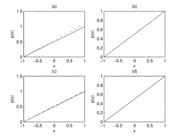
Figure 2. Comparison between the asymptotic solution and the numerical solution of Eq.(43) for small $\varepsilon$. (a) $\alpha=0.5,\varepsilon=0.01$. The asymptotic solution is shown with dashed line while the numerical solution is displayed with solid line. (b) $\alpha=1.5,\varepsilon=0.01$. (c) $\alpha=0.5,\varepsilon=0.001$. (d) $\alpha=1.5,\varepsilon=0.001$.

Figure 2 shows that if $\varepsilon$ is fixed and $\alpha$ turns large, the difference between the asymptotic solution and the numerical solution of Eq.(43) will become small; if $\alpha$ is fixed and $\varepsilon$ becomes large, the difference will turn large, because the asymptotic solution is for sufficiently small $\varepsilon$.

Example 5.2.

For the deterministic dynamical system

$$\dot{x}=x(1-\theta x)-\beta\frac{x}{x+1},$$

where $0<\theta<1$, $1<\beta<\frac{(\theta+1)^{2}}{4\theta}$ and the potential function is

$$U(x)=-\frac{x^{2}}{2}+\frac{\theta x^{3}}{3}+\beta x-\beta\ln(x+1),$$

$x$ is the normalized molecular density of tumor cells with respect to the maximum tissue capacity ([3]). The system has two stable states and one unstable state:

$$x_{1}=0,$$

$$x_{2}=\frac{1-\theta-\sqrt{(1-\theta)^{2}-4\theta(\beta-1)}}{2\theta},$$

$$x_{3}=\frac{1-\theta+\sqrt{(1-\theta)^{2}-4\theta(\beta-1)}}{2\theta}.$$

Without random fluctuations, system states finally approach one of the two stable states: (i) either the stable state $x_{1}=0$, where no tumor cells are present, namely, the tumor-free state (or the state of tumor extinction), (ii) or the other stable state $x_{3}$, where the tumor cell density does not increase but stays at a certain constant level, namely, the state of stable tumor.

Under the environment fluctuations, the tumor density is described by the following scalar SDE with a symmetric $\alpha$-stable Lévy motion, with $1<\alpha<2$,

$$\left\{\begin{array}[]{l}\mathrm{d}X_{t}=\left[X_{t}(1-\theta X_{t})-\beta\frac{X_{t}}{X_{t}+1}\right]\,\mathrm{d}t+\varepsilon\mathrm{d}L_{t}^{\alpha},\\ X_{0}=x.\end{array}\right.$$

The unique solution is denoted as $X_{t}(x)$. We take $(A,B)=(x_{1},x_{3})$ and $(-\infty,A]=(-\infty,x_{1}]$. The escape probability $p(x)$, for $X_{t}(x)$ from $(x_{1},x_{3})$ to $(-\infty,x_{1}]$, i.e. the likelihood of tumor extinction, satisfies the following integro-differential equation

$$\left[x(1-\theta x)-\beta\frac{x}{x+1}\right]p^{\prime}(x)+\varepsilon^{\alpha}\int_{{\mathbb{R}}\setminus\{0\}}\left(p(x+u)-p(x)-p^{\prime}(x)u\right)\nu(\mathrm{d}u)=0,$$

$$x\in(x_{1},x_{3}),$$

with the exterior conditions

$$p(x)|_{(-\infty,x_{1}]}=1,\qquad p(x)|_{[x_{3},\infty)}=0.$$

Since $b(x)=x(1-\theta x)-\beta\frac{x}{x+1},b(x_{2})=0,b^{\prime}(x_{2})>0$, by the result of Case 3 in Section 4, an asymptotic solution of $p(x)$ is given by

$$p(x)\approx\bar{H}\left(\frac{x-x_{2}}{\varepsilon}\right),$$

where $\bar{H}(x)$ solves the following equation

$$b^{\prime}(x_{2})\eta\bar{H}^{\prime}(\eta)+\int_{{\mathbb{R}}\setminus\{0\}}\big{(}\bar{H}(\eta+u)-\bar{H}(\eta)-\bar{H}^{\prime}(\eta)u\big{)}\nu(\mathrm{d}u)=0,$$

with the matching conditions

$$\lim\limits_{\eta\rightarrow-\infty}\bar{H}(\eta)=1,$$

$$\lim\limits_{\eta\rightarrow\infty}\bar{H}(\eta)=0.$$

Example 5.3.

Consider the following scalar SDE with a symmetric $\alpha$-stable Lévy motion, with $1<\alpha<2$,

$$\left\{\begin{array}[]{l}\mathrm{d}X_{t}=-X_{t}\,\mathrm{d}t+\varepsilon\mathrm{d}L_{t}^{\alpha},\\ X_{0}=x.\end{array}\right.$$

The unique solution is denoted as $X_{t}(x)$. We take $(A,B)=(-1,1)$ and $[B,\infty)=[1,\infty)$. The escape probability $p(x)$, for $X_{t}(x)$ from $(-1,1)$ to $[1,\infty)$, satisfies the following integro-differential equation

$$-xp^{\prime}(x)+\varepsilon^{\alpha}\int_{{\mathbb{R}}\setminus\{0\}}\left(p(x+u)-p(x)-p^{\prime}(x)u\right)\nu(\mathrm{d}u)=0,$$

$$x\in(-1,1),$$ (48)

with the exterior conditions

$$p(x)|_{(-\infty,-1]}=0,\qquad p(x)|_{[1,\infty)}=1.$$ (49)

Since $b(x)=-x,b(0)=0,b^{\prime}(0)<0,b(-1)b(1)=-1\neq 0$, by the result of Case 4 in Section 4, an asymptotic solution of $p(x)$ is given by

$$p(x)\approx C\cdot F\left(\frac{x+1}{\varepsilon^{\frac{\alpha}{\alpha-1}}}\right)+(1-C)\cdot G\left(\frac{1-x}{\varepsilon^{\frac{\alpha}{\alpha-1}}}\right).$$ (50)

Specially, take the Lévy measure

$$\nu(\mathrm{d}u)=\frac{\kappa}{|u|^{1+\alpha}}\cdot 1_{|u|\leqslant 1}\mathrm{d}u,$$

where $\kappa>0$ is a constant([15]). Thus, the function $F$ can be given explicitly by

$$F(x)=\left\{\begin{array}[]{l}1-e^{-\gamma x},\quad x>0,\\ 0,\qquad\qquad x\leqslant 0,\end{array}\right.$$

where $\gamma>0$ satisfies the following integral equation

$$\gamma-\int_{-1}^{1}\left(e^{-\gamma u}-1-(-\gamma)u\right)\frac{\kappa}{|u|^{1+\alpha}}\mathrm{d}u=0.$$

By the relation between $F$ and $G$, we can obtain

$$G(x)=\left\{\begin{array}[]{l}e^{-\gamma x},\qquad x>0,\\ 1,\qquad\quad x\leqslant 0.\end{array}\right.$$

So, the asymptotic solution of Eq.(48) is given by

$$p(x)\approx C\left(1-\exp\left\{-\gamma\left(\frac{x+2}{\varepsilon^{\frac{\alpha}{\alpha-1}}}\right)\right\}\right)+(1-C)\exp\left\{-\gamma\left(\frac{1-x}{\varepsilon^{\frac{\alpha}{\alpha-1}}}\right)\right\}.$$

To determine $C$, we multiply Eq.(48) by the solution $\rho(x)$ of the steady Fokker-Planck equation

$$-(-x\rho(x))^{\prime}+\varepsilon^{\alpha}\int_{{\mathbb{R}}\setminus\{0\}}\left(\rho(x+u)-\rho(x)-\rho^{\prime}(x)u\right)\nu(\mathrm{d}u)=0$$ (51)

and integrate over $(-1,1)$, to obtain

$$\int_{-1}^{1}\big{(}-x\rho(x)\big{)}p^{\prime}(x)\mathrm{d}x+\varepsilon^{\alpha}\int_{-1}^{1}\rho(x)\mathrm{d}x\int_{{\mathbb{R}}\setminus\{0\}}\left(p(x+u)-p(x)-p^{\prime}(x)u\right)\nu(\mathrm{d}u)=0.$$ (52)

To (52), by integration by parts and using (51), we get

$$-\rho(1)-\varepsilon^{\alpha}\int_{-1}^{1}p(x)\mathrm{d}x\int_{{\mathbb{R}}\setminus\{0\}}\left(\rho(x+u)-\rho(x)-\rho^{\prime}(x)u\right)\nu(\mathrm{d}u)$$

$$+\varepsilon^{\alpha}\int_{-1}^{1}\rho(x)\mathrm{d}x\int_{{\mathbb{R}}\setminus\{0\}}\left(p(x+u)-p(x)-p^{\prime}(x)u\right)\nu(\mathrm{d}u)=0.$$

Applying Cauchy principal value and (49), we have

$$-\frac{\varepsilon^{-\alpha}\rho(1)}{C_{1,\alpha}}+\int_{-1}^{1}\rho(x)\frac{(1-x)^{-\alpha}}{\alpha}\mathrm{d}x$$ (53)

$$= \int_{-1}^{1}p(x)\mathrm{d}x\left[\int_{-\infty}^{-1}\frac{\rho(y)}{|y-x|^{1+\alpha}}\mathrm{d}y+\int_{1}^{\infty}\frac{\rho(y)}{|y-x|^{1+\alpha}}\mathrm{d}y\right].$$

By [1, Proposition 3.2], the Fourier transform of $\rho(k)$ is given by

$$\hat{\rho}(k)=\exp\{-\frac{\varepsilon^{\alpha}}{\alpha}|k|^{\alpha}\}.$$

Replacing $\rho(x)$ and $p(x)$ by $\frac{1}{2\pi}\int_{{\mathbb{R}}}e^{ixk}\hat{\rho}(k)\mathrm{d}k$ and (50), respectively, and letting $\varepsilon\rightarrow 0$, we can obtain $C$ from (53).

Acknowledgement. We thank Xingye Kan for help with Example 5.1. This work was done while Huijie Qiao was visiting the Institute for Pure and Applied Mathematics (IPAM), Los Angeles.

References

• [1] S. Albeverio, B. Rüdiger and J. Wu: Invariant measures and symmetry property of Lévy type operators, Potential Analysis, 13(2000)147-168.
• [2] D. Applebaum: Lévy Processes and Stochastic Calculus, Second Edition, Cambridge Univ. Press, Cambridge, 2009.
• [3] A. Fiasconaro, A. Ochab-Marcinek, B. Spagnolo and E. Gudowska- Nowak, Monitoring noise-resonant effects in cancer growth influenced by external fluctuations and periodic treatment, Eur. Phys. J. B, 65 (2008)435-442.
• [4] T. Gao, J. Duan, X. Li and R. Song, Mean exit time and escape probability for dynamical systems driven by Lévy noise. Submitted to Methodology and Computing in Applied Probability, 2011.
• [5] N. Jacob: Pseudo Differential Operators and Markov Processes, Volume II, Generators and Their Potential Theory, Imperial College Press, 2002.
• [6] J. K. Kevorkian and J. D. Cole: Multiple Scale and Singular Perturbation Methods, Applied Mathematical Sciences 114, Springer-verlag, New York, 1996.
• [7] T. Koren, A. V. Chechkin and J. Klafter: On the first passage time and leapover properties of Lévy motions, Physica A 379, (2007)10-22.
• [8] M. Liao: The Dirichlet problem of a discontinuous Markov process, Acta Mathematica Sinica, 5(1989)9-15.
• [9] B. Matkowsky, Z. Schuss, and C. Tier, Asymptotic Methods for Markov Jump Processes, A. M. S. Lectures in Applied Mathematics 27, 1991, p. 215-240.
• [10] H. Qiao, X. Kan and J. Duan: Escape probability for stochastic dynamical systems with jumps, appear in Nualart’s Festschrift.
• [11] H. Qiao and X. Zhang: Homeomorphism flows for non-Lipschitz stochastic differential equations with jumps, Stochastic Processes and their Applications, 118(2008)2254-2268.
• [12] K. Sato: Lévy processes and infinitely divisible distributions, Cambridge University Press, 1999.
• [13] Z. Schuss, Theory and Applications of Stochastic Differential Equations, Wiley & Sons, New York, 1980.
• [14] H. Tanaka, M. Tsuchiya and S. Watanabe: Perturbation of drift-type for Lévy processes, J. Math. Kyoto Univ., 14(1974)73-92.
• [15] W. A. Woyczynski, Lévy processes in the physical sciences. In Lévy Processes: Theory and Applications, O. E. Barndorff-Nielsen, T. Mikosch and S. I. Resnick (Eds.), 241-266, Birkhäuser, Boston, 2001.