Radiatively Efficient Magnetized Bondi Accretion

Abstract

We have carried out a numerical study of the effect of large scale magnetic fields on the rate of accretion from a uniform, isothermal gas onto a resistive, stationary point mass. Only mass, not magnetic flux, accretes onto the point mass. The simulations for this study avoid complications arising from boundary conditions by keeping the boundaries far from the accreting object. Our simulations leverage adaptive refinement methodology to attain high spatial fidelity close to the accreting object. Our results are particularly relevant to the problem of star formation from a magnetized molecular cloud in which thermal energy is radiated away on time scales much shorter than the dynamical time scale. Contrary to the adiabatic case, our simulations show convergence toward a finite accretion rate in the limit in which the radius of the accreting object vanishes, regardless of magnetic field strength. For very weak magnetic fields, the accretion rate first approaches the Bondi value and then drops by a factor $\sim 2$ as magnetic flux builds up near the point mass. For strong magnetic fields, the steady-state accretion rate is reduced by a factor $\sim 0.2\beta^{1/2}$ compared to the Bondi value, where $\beta$ is the ratio of the gas pressure to the magnetic pressure. We give a simple expression for the accretion rate as a function of the magnetic field strength. Approximate analytic results are given in the Appendixes for both time-dependent accretion in the limit of weak magnetic fields and steady-state accretion for the case of strong magnetic fields.

1 Introduction

Accretion of a background gas onto a central gravitating body is of central importance in astrophysics. Examples range from protostellar accretion from molecular cores to accretion of interstellar gas in galactic nuclei. The classical late-time solution for the case of a central point of mass $M_{*}$ immersed in a uniform, initially static, unmagnetized gas was given by Bondi (1952) as

$$\dot{M}_{\rm B} = 4\pi\lambda{r_{\rm B}}^{2}\rho_{\infty}c_{\infty}$$ (1)

$${r_{\rm B}} = \frac{GM_{*}}{c^{2}_{\infty}}$$ (2)

where $c_{\infty}$ and $\rho_{\infty}$ are the sound speed and density of the background gas, $\dot{M}_{\rm B}$ is the steady-state rate of accretion onto the central particle, ${r_{\rm B}}$ is the Bondi length which characterizes the dynamical length of the inflow and $\lambda$ is a dimensionless parameter that depends on the equation of state of the background gas. For the isothermal case, $\lambda=\textrm{exp}(1.5)/4$. The Bondi time ${t_{\rm B}}={r_{\rm B}}/c_{\infty}$ defines the dynamical time for this accretion process. This basic model has been extended to more general cases by numerous authors. These generalizations include non-stationary central particles (Bondi & Hoyle, 1944; Shima et al., 1985; Ruffert, 1994; Ruffert & Arnett, 1994), the cases of ambient gas with net vorticity (Krumholz et al., 2005), turbulent ambient gas (Krumholz et al., 2006), magnetized accretion from ambient gas threaded by both large (Igumenshchev & Narayan, 2002; Pang et al., 2011) and small (Shapiro, 1973; Igumenshchev, 2006) scale magnetic field topologies, the case of a turbulent, magnetized ambient gas (Shcherbakov, 2008), and the case of accretion onto magnetized stars (Toropin et al., 1999; Ustyugova et al., 2006; Kulkarni & Romanova, 2008; Romanova et al., 2008; Long et al., 2011; Romanova et al., 2011), to name a few.

Stars form via gravitational collapse, at least initially (McKee & Ostriker, 2007). Thereafter, gas may accrete onto the star from the ambient medium. If the star has a supersonic motion relative to the ambient medium, this subsequent accretion is negligible (Krumholz et al., 2005), but if the star is moving slowly, the accretion can be significant, which forms the basis for the competitive accretion model for star formation (e.g., Bonnell et al., 1997). There exists ample evidence that the gas in molecular clouds and cores is threaded by strong magnetic fields (Crutcher, 1999; McKee & Ostriker, 2007). Furthermore, star forming molecular clouds are well characterized as “radiatively efficient” in that gas heating due to compressional motion is rapidly radiated by thermally excited dust and molecules. These considerations thus motivate the study of Bondi-type accretion of an isothermal gas threaded by an initially uniform magnetic field onto a point mass. We address this problem with the RAMSES magnetohydrodynamic (MHD) code (Teyssier, 2002) and conduct a parameter study over a range of magnetic field strengths thought to be relevant to star formation. Our simulations leverage the adaptive mesh refinement (AMR) capability of the code to retain high spatial resolution close to the accreting object while keeping the boundaries of the computational domain far from the accreting object. We discuss the results of mesh convergence studies and compare our numerical results against analytic calculations in the limiting case of a dynamically weak magnetic field to verify our calculations. We also compare our numerical results against simple analytic approximations in the case of a strong magnetic field.

2 Numerical Setup

Our numerical models consist of a Cartesian computational domain that extends from $-25{r_{\rm B}}~{}\textrm{to}~{}25{r_{\rm B}}$ in each direction. The domain is initialized with an isothermal, perfectly conducting, uniform collisional gas with initial magnetic field in the $\hat{z}$ direction. We consider the cases with an initial thermal to magnetic pressure ratio, $\beta=8\pi P_{o}/{\bf B}^{2}$, of 1000, 100, 10, 1, 0.1 and 0.01. The RAMSES code has been used to evolve this state forward according to the equations of ideal, isothermal MHD,

$$\frac{\partial\rho}{\partial t}+\raise 1.93747pt\hbox{$\bigtriangledown$\hskip-8.62224pt$\bigtriangledown$\hskip-8.62224pt$\bigtriangledown$\hskip-8.62224pt}\raise 2.0236pt\hbox{$\bigtriangledown$}\cdot\rho{\bf v} = -S_{M}$$ (3)

$$\frac{\partial\rho{\bf v}}{\partial t}+\raise 1.93747pt\hbox{$\bigtriangledown$\hskip-8.62224pt$\bigtriangledown$\hskip-8.62224pt$\bigtriangledown$\hskip-8.62224pt}\raise 2.0236pt\hbox{$\bigtriangledown$}\cdot(\rho{\bf v}{\bf v})+\raise 1.93747pt\hbox{$\bigtriangledown$\hskip-8.62224pt$\bigtriangledown$\hskip-8.62224pt$\bigtriangledown$\hskip-8.62224pt}\raise 2.0236pt\hbox{$\bigtriangledown$}\left(P+\frac{{\bf B}^{2}}{8\pi}\right)-\frac{({\bf B}\cdot\raise 1.93747pt\hbox{$\bigtriangledown$\hskip-8.62224pt$\bigtriangledown$\hskip-8.62224pt$\bigtriangledown$\hskip-8.62224pt}\raise 2.0236pt\hbox{$\bigtriangledown$}){\bf B}}{4\pi} = -\frac{GM_{*}\rho~{}\hat{{\bf x}}}{{\bf x}^{2}}$$ (4)

$$\frac{\partial B}{\partial t}-\raise 1.93747pt\hbox{$\bigtriangledown$\hskip-8.62224pt$\bigtriangledown$\hskip-8.62224pt$\bigtriangledown$\hskip-8.62224pt}\raise 2.0236pt\hbox{$\bigtriangledown$}\times({\bf v}\times{\bf B}) = 0$$ (5)

$$P = \rho c^{2},$$ (6)

where $\rho$ is the gas density, ${\bf v}$ is the velocity, ${\bf B}$ is the magnetic field, $P$ is the thermal pressure and $c$ is the isothermal sound speed. These equations include the gravitational force due to a point particle of mass $M_{*}$ of ${\bf F}_{g}=-GM_{*}\rho~{}\hat{{\bf x}}/{\bf x}^{2}$.

The key assumption we make in our treatment is that the point mass accretes mass, but not flux. Observations show that the magnetic flux in young stellar objects is orders of magnitude less than that in the gas that formed these objects, implying that flux accretion is very inefficient, presumably due to non-ideal MHD effects, including reconnection (McKee & Ostriker, 2007). We model mass accretion onto the central point mass by including a mass sink term but no flux sink term inside a radius, $r_{\rm acc}=4\Delta x$, equal to four grid zones on the finest AMR level. The effect of the accreting particle is coupled to the dynamical equations through the source term,

$$S_{M}=\left\{\begin{array}[]{ll}\displaystyle\frac{1}{\Delta t}\,\textrm{max}\left(\rho-\frac{{\bf B}^{2}}{4\pi v_{\rm A,max}^{2}}\,,\,0\right)&\textrm{if ~{}}|{\bf x}|<r_{\rm acc}\\ 0&\textrm{otherwise,}\end{array}\right.$$ (7)

where $\Delta t$ is the time step on the finest AMR grid level and $v_{\rm A,max}$ is the maximum Alfv$\acute{\rm e}$n speed, $B/(4\pi\rho)^{1/2}$, within a radius of $6\Delta x$ around the accreting particle. Under this construction, the accreting particle absorbs all but enough of the mass entering the accreting particle radius so that the local Alfv$\acute{\rm e}$n speed never exceeds $v_{\rm A,max}$. Thus, the accreting particle always absorbs the largest quantity of mass in the local region possible without introducing new local extrema in the Alfv$\acute{\rm e}$n speed. This prevents the accretion source from imposing a stringent (or vanishingly small) constraint on the maximum numerically stable time-step at the expense of some artificial clipping of the Alfv$\acute{\rm e}$n speed in the inner few zones around the accreting particle. We note that in all of the models considered in this paper, the initial gas density is sufficiently low that the total mass accreted onto the central particle is negligible compared to $M_{*}$ and that self-gravity in the ambient medium may be neglected.

We discretize the numerical domain onto a base level grid of $64^{3}$. For the purposes of describing the initial mesh we will denote this level as $l=0$. We note, however, that the RAMSES AMR implementation uses an oct-tree data structure for level traversals that always denotes level indices by the base 2 logarithm of their resolution. In our models, $l_{\rm RAMSES}=\textrm{log}_{2}64+l=6+l$. Successive levels are chosen for refinement by an increment of $2^{3}$ in grid zone density in a geometrically nested fashion according to the criterion

$$r_{l}<\frac{25{r_{\rm B}}}{2^{l}},$$ (8)

where $r_{l}$ indicates the radius of the spherical refined region on the level $l$. We further impose the additional criterion that any zones containing steep density gradients ${\bf\raise 1.93747pt\hbox{$\bigtriangledown$\hskip-8.62224pt$\bigtriangledown$\hskip-8.62224pt$\bigtriangledown$\hskip-8.62224pt}\raise 2.0236pt\hbox{$\bigtriangledown$}}\rho\cdot{\bf\Delta x}/\rho>1/2$ are also refined, independent of location. This second refinement criterion is met only at late times after non-axisymmetric flow patterns have set in, and it triggers only on transient flow features. Most of the models were refined to a maximum level $l=8$ for an effective resolution of $64\times 2^{8}/50\simeq 328$ zones per thermal Bondi radius on the finest level. In the cases with a strong initial magnetic field, it is also useful to consider the numerical resolution on the scale of the “Alfv$\acute{\rm e}$n-Bondi” radius,

$$r_{\rm AB}=\frac{GM_{*}}{v_{\rm A}^{2}}=\frac{1}{2}\beta{r_{\rm B}}.$$ (9)

The finest mesh resolution per Bondi radius, mesh resolution per Alfv$\acute{\rm e}$n-Bondi radius and total simulated time for each model is tabulated in Table 1. We note that the magnetic length scales are well resolved for all but the case of $\beta=0.01$. We therefore will consider only the models with $\beta\geq 0.1$ for the majority of the analysis presented in this paper. The $\beta=0.01$ model is used only to extract an estimate of the steady accretion rate over a wider range of magnetic field strengths. We do note, however, that numerical mesh convergence studies have shown our models to be within the range of asymptotic convergence with a Richardson-extrapolation error estimate on the average accretion rate of $14\%$ or less at late times. A detailed discussion of the numerical convergence properties of our models is presented in Appendix A. Each of the models were run to a final time $t_{\rm end}$ sufficiently long to attain a statistically steady accretion rate onto the central particle.

Table 1: Simulation Parameters.

$\beta$	$r_{\rm B}/\Delta x$	$r_{\rm AB}/\Delta x$	$t_{\rm end}/{t_{\rm B}}$
$\infty$ (hydro)	328	N/A	3
1000	82	41000	22
100	82	4100	15
10	328	1640	3
1	328	164	3
0.1	328	16.4	3
0.01	328	1.64	1.5

3 Results

3.1 Morphology

We begin by discussing the gross morphological flow features and their development for each of the numerical models. These flows are well illustrated by slices in the y-z plane of density, the direction of magnetic flux and velocity as shown at several times for each model in Figure 1. Initially parallel magnetic fields are amplified as they are dragged inward by the global accretion flow, eventually suppressing accretion in the equatorial plane. Inflow along magnetic field lines, on the other hand, is uninhibited by magnetic pressure. This flow configuration leads to the evacuation of gas from the poleward directions into a thin, dense, irrotational disk in the midplane.

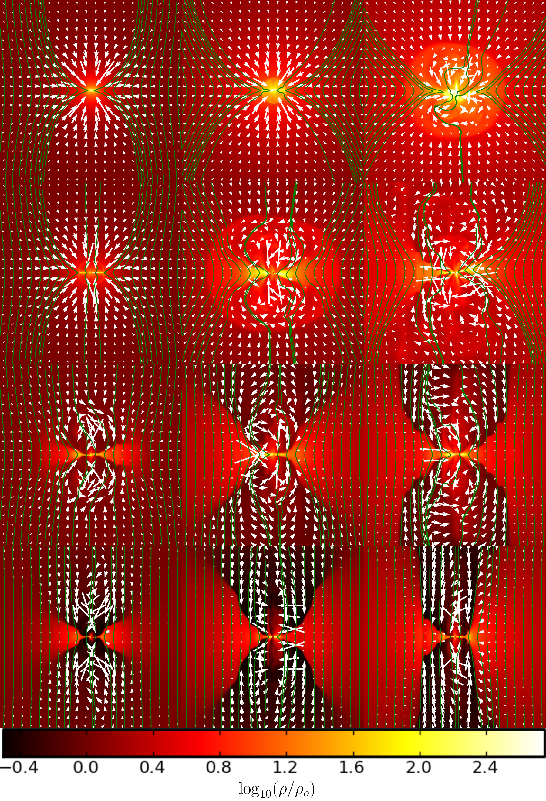
Figure 1: Slices in the y-z plane showing the inner $(2{r_{\rm B}})^{2}$ of the numerical models with initial magnetic field strengths of $\beta=100$, $\beta=10$, $\beta=1$, and $\beta=0.1$ from top to bottom. The state of the numerical models are shown at the times $t=0.5,~{}1.5,~{}\textrm{and}~{}3.0~{}{t_{\rm B}}$ from left to right. The colormap indicates $\log_{10}(\rho/\rho_{o})$, green lines represent magnetic flux tubes drawn from equidistant foot-points in the midplane and the white arrows indicate the flow pattern in the plane of the slice.

Accumulation of mass in the midplane is accompanied by a corresponding increase in the inward gravitational attraction. The magnetic flux tubes that thread the disk are gradually pulled further toward the accreting particle as the accumulation of mass in the midplane continues. We support this picture more quantitatively in Figure 2. We use $\varpi$ to denote the cylindrical radius and plot the ratio of the mass influx in the equatorial direction

$$\Phi_{M,\varpi}=\int_{S}\rho{\bf v}\cdot\hat{\varpi}\sin\theta d\theta d\phi$$ (10)

to the mass influx in the polar direction

$$\Phi_{M,z}=\int_{S}\rho{\bf v}\cdot\hat{{\bf z}}\sin\theta d\theta d\phi$$ (11)

along a spherical control surface $S$ of radius $r$ for each of the magnetized models at $t=t_{\rm end}$. The curves in Figure 2 have been scaled by a constant $2/\pi$ so that uniform spherical inflow takes a value of unity. At large distances ($|{\bf x}|>{r_{\rm B}}$), the flows become increasingly dominated by polar inflow with increasing initial magnetic field strength. However, at smaller distances ($|{\bf x}|<{r_{\rm B}}$), the cylindrical to polar influx asymptotes toward $\sim 2$ with increasing magnetic field strength. On smaller scales where magnetic forces break spherical symmetry, the mass influx is predominantly along the equator.

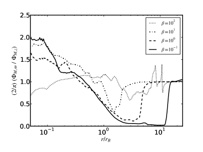
Figure 2: The ratio of the mass influx in the equatorial direction to the mass influx in the polar direction for several magnetized models at $t=t_{\rm end}$, scaled so that uniform spherical inflow takes a value of unity.

As infall in the midplane proceeds, flux tubes that reach the accreting particle are instantaneously liberated from the accreted mass and accompanying gravitational force anchoring them. This causes episodic releases of strong, outward propagating flow. This configuration of outflow driven by magnetic buoyancy is known as the magnetic interchange instability (Bernstein et al., 1958; Furth et al., 1963). In the models with moderate or strong initial magnetic fields strengths, corresponding to $\beta=10$, $\beta=1$ and $\beta=0.1$, interchange unstable flows originating at $r_{acc}\ll{r_{\rm B}}$ lead to episodes of net outflow out to radii comparable ${r_{\rm B}}$ in the equatorial plane. Flux tubes that are outwardly released by resistive accretion are prevented from escaping completely by the continued accretion pressure of the surrounding gas. The net mass inflow in these models is therefore mediated by the rate at which inflowing material percolates through this non-axisymmetric network of magnetically buoyant flow close to the accreting particle.

The models attain magnetic forces that balance $F_{g}$ at $r\sim{r_{\rm B}}/2$ in the midplane by the time steady accretion sets in, independent of the initial $\beta$. The weak magnetic field lines in the $\beta=100$ case become highly stretched before they are strong enough to provide any resistance to being swept further inward as shown in the top row of Figure 1. This flow leads to the development of strong, thin current sheets and oppositely directed magnetic field lines that closely approach each other in the midplane. This configuration is unstable to reconnection in magnetic resistive tearing modes (Furth et al., 1963; Rutherford, 1973). In the case of our numerical code (and all ideal MHD codes), resistive reconnection occurs when oppositely directed magnetic flux tubes become separated by $\lesssim\Delta x$ and unresolved. While the size scale of the “magnetic islands” generated through this process is determined by the numerical zone size, our numerical resolution is adequate to be sure that this size scale is small compared to dynamical scale associated with thermal ($\Delta x\ll r_{\rm B}$) and magnetic ($\Delta x\ll r_{\rm AB}$) force gradients. Furthermore, we have carried out resolution studies to ensure that the resoultion used in our models is sufficient to yield a converged late-time accretion rate. Ultimately, mass inflow is limited by the rate of production of magnetically isolated islands by tearing mode reconnection in regions characterized by thin, strong current sheets. These islands continue toward the accreting particle, unconnected to the global magnetic field structure. As a means to visualize flows that are most susceptible to reconnection by numerical resistivity, we define the magnetic shear parameter

$$\chi_{\rm mag}=\frac{\Delta{\bf x}\cdot(\raise 1.93747pt\hbox{$\bigtriangledown$\hskip-8.62224pt$\bigtriangledown$\hskip-8.62224pt$\bigtriangledown$\hskip-8.62224pt}\raise 2.0236pt\hbox{$\bigtriangledown$}\times{\bf B})}{|{\bf B}|}.$$ (12)

Regions near or exceeding a magnetic shear parameter of $\sim 1$ are highly susceptible to reconnection via magnetic tearing modes. Figure 3 gives a three dimensional sense of the geometry and scale of the flows subject to numerical reconnection by plotting isosurfaces of the magnetic shear parameter at $t=t_{\rm end}$, indicating efficient numerical reconnection on scales of $r\lesssim{r_{\rm B}}/2$. Reconnection events release magnetic tension that leads to magnetically tangled, non-axisymmetric flow in this region.

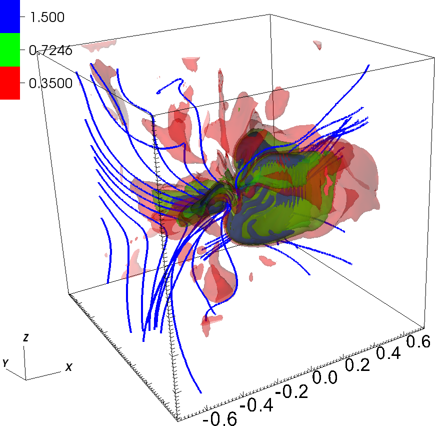
Figure 3: Isosurfaces showing the innmermost $(1.5{r_{\rm B}})^{3}$ of the magnetic shear parameter $\chi_{\rm mag}$ at $t=t_{\rm end}$ for the $\beta=100$ model indicating regions of magnetic reconnection due to tearing mode instability. Blue curves represent magnetic field lines with footpoints evenly spaced along the y coordinate axis.

3.2 Comparison to Analytic Predictions for High $\beta$ Flow

Analytic predictions of the behavior of the accretion flows for the limiting case of dynamically weak magnetic field are derived in appendix B. The focus of this section is to compare the results of the $\beta=100$ numerical model with these analytic predictions. Equations (B16), (B23) and (B25) give predictions of the steady state gas density, radial magnetic field and non-radial magnetic field respectively. (Results for the accretion rate will be discussed in §3.3) It should be emphasized that $r_{0}$ in these expressions is the initial position of gas that is at $r$ at time $t$, and it must be evaluated numerically through the transcendental equation (B8). In Figure 4 we compare these analytic predictions to the results of each of the magnetized numerical models at $t=t_{\rm end}$. The gas density, $\rho$, and the non-radial magnetic field, $B_{\theta}$, are extracted from the numerical models as azimuthal averages in the midplane of the numerical domain where the sine term appearing in equation (B25) is unity. Likewise, the radial magnetic field $B_{r}$ is extracted from the numerical models along the $x=y=0$ axis where the cosine term in equation (B23) is unity. The assumption of dynamically weak magnetic field is met for $r\gtrsim{r_{\rm B}}$ in the $\beta=1000$ model and we find good agreement between the $\beta=1000$ model and the analytic prediction at distances not too close to the origin. The analytic theory also agrees with the results for stronger fields for $r\lower 2.15277pt\hbox{$\;\buildrel>\over{\sim}\;$}4{r_{\rm B}}$.

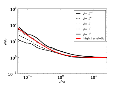
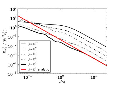
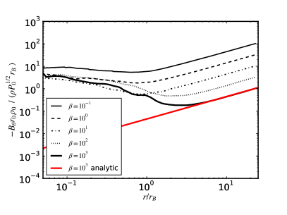
Figure 4: Top Left: Azimuthally averaged density in the $z=0$ plane. Top Right: Azimuthally averaged radial component of the magnetic field in the $z=0$ plane, scaled inversely to the square of $r_{0}$. Bottom Left: Perpendicular component of the magnetic field along the $x=0,~{}y=0$ axis, scaled by $r_{0}$ and inversely to the density. Each plot shows the analytic prediction for the limiting case of weak magnetic field with $\beta=1000$. All of the plots are taken at time $t=t_{\rm end}$.

In appendix B.1, equation (B.2.2), we derive an analytic prediction for the total magnetic flux that reaches the accretion zone, $\Phi_{a}$, under the assumption of dynamically weak magnetic fields and neglecting any possible reconnection that occurs near the accretion zone. We have assumed that this flux escapes from the accretion zone. Even with reconnection, this method accurately tracks the amount of escaping flux, although the time at which the flux escapes may be altered by the reconnection. Let $\Phi_{\rm esc}(r)$ be the magnetic flux that is inside a radius $r$ and that has escaped from the accretion zone. This quantity is well defined only for ideal MHD, so that $r$ must be outside the region where magnetic reconnection occurs. At large values of $r$, $\Phi_{\rm esc}(r)\rightarrow\Phi_{a}$, the total flux released during accretion. As discussed above, reconnection occurs in the inner regions of the flow, where it becomes very turbulent. Outside this region, the flow is approximately axisymmetric. There we can define $r_{0}$ as the initial radius of the gas and magnetic flux, which at time $t$ is located in the midplane at radius $r<r_{0}$. The initial flux inside $r_{0}$ is then the sum of the flux inside $r(r_{0})$ plus the flux that has escaped beyond $r$,

$$\Phi_{0}[r_{0}(r)]=\Phi(r)+[\Phi_{a}-\Phi_{\rm esc}(r)],$$ (13)

where $\Phi_{0}[r_{0}(r)]=|{\bf B_{o}}|\pi r_{0}^{2}$. Equation (B8) gives $t$ as a function of $r$ and $r_{0}$; this can be inverted numerically to obtain $r_{0}(r,t)$. We note that equation (13) applies only outside the reconnection zone. If we had not assumed that the flux could escape from the accretion zone after losing some of its mass, flux would be conserved and both $\Phi_{a}$ and $\Phi_{\rm esc}$ would vanish.

We can use our numerical models to test the predicted value of $\Phi_{a}$ and to determine the radial distribution of the escaped flux. To do this, we extract $\Phi(r)$ from our numerical result at a late time ($t=15{t_{\rm B}}$), and we compare to the analytic result by rewriting equation (13) as

$$\delta_{\Phi}=\frac{\Phi_{a}-\Phi_{\rm esc}(r)}{\Phi_{0}[r_{0}(r)]}=1-\frac{\Phi(r)}{\Phi_{0}[r_{0}(r)]},$$ (14)

which is the fraction of the escaped flux that is beyond $r$. In the left panel of Figure 5 we show the above expression for the high $\beta$ models. In this case, the assumption of dynamically weak magnetic fields used to derive the analytic estimate for $r(r_{0})$ is well met at $r\lower 2.15277pt\hbox{$\;\buildrel>\over{\sim}\;$}{r_{\rm B}}$. We expect that $\Phi(r)\approx\Phi_{0}[r_{0}(r)]$ for $r\gg{r_{\rm B}}$, and this is confirmed to within $10\%$ for $r>4{r_{\rm B}}$. Given our assumption of a resistive accreting particle, we expect that $\Phi(r)\rightarrow 0$ as $r\rightarrow 0$, and Figure 5 confirms this expectation by showing $\delta_{\Phi}\rightarrow 1$ as $r\rightarrow 0$. Furthermore, the accumulated flux near the accreting particle shows strong evidence of escape for $r\lesssim 1$, consistent with the scale of reconnection-driven tearing modes shown in Figure 3 and discussed in section §3.1. The fact that $\delta_{\Phi}$ is greater than unity at large radii is presumably due to the approximation made in determining $r_{0}(r)$. In the case of $\beta=100$, it appears that a significant fraction of the escaped flux ($\lower 2.15277pt\hbox{$\;\buildrel>\over{\sim}\;$}20\%$) has moved outside ${r_{\rm B}}$.

In appendix B.1 we also predict the radius $r_{\Phi}$ out to which the magnetic forces associated with the accumulated flux strongly affect the flow. The analytic estimate of $r_{\Phi}$ for high $\beta$ flow is given by equation (B39). In the right panel of Figure 5, we plot this prediction against the radius where the median plasma $\beta$ exceeds unity along the perimeter of a control circle in the midplane of the high $\beta$ models. At the latest time shown, the prediction agrees with the simulation to within about 20% for the $\beta=100$ case. Note that at late times, the analytic approximation has $r_{\Phi}\propto t^{1/3}$, but it is not known whether the numerical results will continue to increase for $t>t_{\rm end}$. It is not entirely clear why the $\beta=1000$ results do not agree with the approximate model as well as the $\beta=100$ results. The model predicts that $r_{\Phi}$ should be very close to (and slightly less than) $r_{\Phi,1}$, given by equation (B35) for $\beta=1000$, whereas the simulations show that it is between $r_{\Phi,1}$ and $r_{\Phi,2}$, given by equation (B38). This may be associated with the fact that the escaped flux has gone well beyond the sonic point at $t_{\rm end}$ for $\beta=1000$ (see the left-hand panel of Figure 5), so that the conditions are closer to those assumed in deriving $r_{\Phi,2}$ than for $r_{\Phi,1}$.

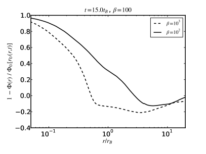
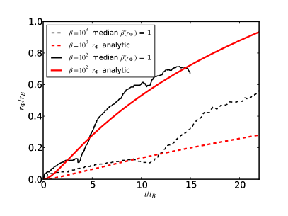
Figure 5: Left: Radial distribution of escaped flux in the $\beta=100$ and $\beta=1000$ models at time $t_{\rm end}$. Right: The radial extent of the magnetically dominated region compared to the analytic prediction.

3.3 Accretion Rate

Figure 6 shows the rate of accretion onto the central particle as a function of time for each of the numerical models. The left plot also includes the result of a purely hydrodynamic control model for comparison. As discussed in §3.1, the magnetized models reach a statistically steady accretion rate with inflow mediated by reconnection and/or the interchange instability, whereas the purely hydrodynamic model asymptotically approaches the truly steady, spherical Bondi flow. The high frequency modes in Figure 6 have been smoothed using a box-car smoothing width of $0.02{t_{\rm B}}$. The red dashed curve shows the analytic approximation for the time-dependent accretion rate without magnetic fields from appendix B.1, equation (B15). The analytic estimate is in excellent agreement with the purely hydrodynamic numerical model.

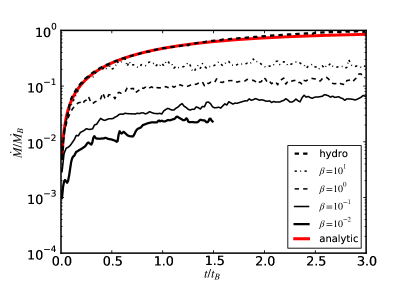
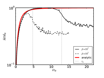
Figure 6: Accretion rate as a function of time for each of the numerical models compared to the analytic prediction for the time-dependent accretion rate for the purely hydrodynamic case. In the right plot the time $t_{\rm ss}$ indicated by a gray vertical line when the accretion rate is midway between the maximum accretion rate and the final steady state accretion rate, representing the characteristic time for the flow to transition from Bondi accretion to a magnetically mediated steady state.

An interesting aspect of the results shown in Figure 6 is that the weak magnetic field models ($\beta=100$ & $\beta=1000$) undergo an initial transient of rapid accretion before settling into a steady accretion rate. The reason for this is that enough time must elapse for sufficient magnetic flux to accumulate close to the accreting particle for the accretion to the surface of the particle to become magnetically dominated, whereas thermal pressure dominates close to the particle during the initial development of the flow. We can use equation (B8) to estimate the time required for the flow to settle into a magnetically mediated steady state accretion regime. Specifically, we estimate the time to reach this steady state, $t_{\rm ss}$, as the time required for enough magnetic flux to accumulate inside the thermal sonic radius, $r_{\rm sonic}={r_{\rm B}}/2$ (Bondi, 1952), so that the average magnetic field within $r<r_{\rm sonic}$ in the midplane corresponds to $\beta=1$ (i.e., $\bar{B}=(8\pi\rho_{0}c^{2})^{1/2}$ for $r<r_{\rm sonic}$ at $t=t_{\rm ss}$). Neglecting any flux that has escaped beyond $r_{\rm sonic}$, this then implies

$$\pi r_{0}(r=r_{\rm sonic},t=t_{\rm ss})^{2}=\pi r_{\rm sonic}^{2}\beta^{1/2}$$ (15)

Solving this for $t_{\rm ss}$ using the transcendental expression for $r_{0}$ in equation (B8) determines $t_{\rm ss}(\beta)$, as shown in Figure 7. The simulations match with this prediction with the $\beta=100$ and $\beta=1000$ models transitioning toward the magnetically dominated steady state accretion rate at $t\sim t_{\rm ss}$ as shown in Figure 6.

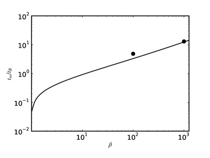
Figure 7: An analytic estimate of the time required for enough magnetic flux to accumulate inside of the thermal sonic radius for the flow to reach a state of magnetically mediated accretion. Black circles indicating the time when the $\beta=10^{2}$ and $\beta=10^{3}$ simulations transition from Bondi to magnetically mediated flow are in good agreement with the analytic prediction.

Figure 8 shows the average accretion rate over the last $t_{\rm B}$ of the simulated time for each of the $\beta=10^{-1}$ - $\beta=10^{3}$ models as black circles. The $\beta=10^{-2}$ model was run only to $t_{\rm end}=1.5t_{\rm B}$ and for that case we average over the last $t_{\rm B}/2$ of the simulated time. The vertical bars on each point indicate the standard deviation of the accretion rate over the same time interval. It should be noted that these should be interpreted as a measure of the effect of small scale departure from steady accretion flow due to MHD flow instability and not as “error bars” in the usual sense of measurement uncertainty. The accretion rate data are presented in tabular form as well in Table 2.

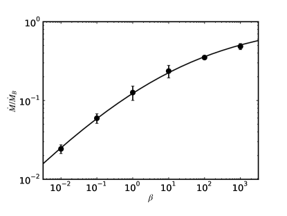
Figure 8: Average accretion rate as a function of plasma $\beta$ parameter. Error bars show the standard deviation in the accretion rate due to interchange and tearing mode unstable flows near the accreting particle. The solid line shows equation (17) with the best-fit coefficients $\beta_{\rm ch}=5.0$ and $n=0.42$.

Table 2: Accretion Rates.

$\beta$	$\dot{M}/\dot{M_{\rm B}}$	$\sigma_{\dot{M}}/\dot{M_{\rm B}}$
1000	0.48	0.043
100	0.35	0.015
10	0.24	0.043
1	0.13	0.26
0.1	0.060	0.083
0.01	0.024	0.031

Note. — Second column: Normalized mean accretion rate for the isothermal equation of state models. Third column: Standard deviation of the isothermal accretion rate.

We can obtain a simple analytic model for the accretion flow in the magnetically dominated case by assuming that the gas flows in from the Alfv$\acute{\rm e}$n radius $r_{\rm AB}$ at the Alfv$\acute{\rm e}$n velocity after collapsing vertically from a distance of order the Bondi radius, ${r_{\rm B}}$:

$$\dot{M}\propto 2\pi r_{\rm AB}\cdot 2r_{\rm AB}\cdot\rho_{\infty}v_{\rm A}\propto\dot{M}_{\rm B}(c/v_{\rm A})\propto\dot{M}_{\rm B}\beta^{1/2}~{}~{}~{}~{}(\beta\ll 1),$$ (16)

where the second expression follows from equation (B17). We note that Toropin et al. (1999) have shown similar accretion rate dependence with magnetic pressure close to the accreteor for the case of the accretion onto a magnetized star. We estimate of the constant of proportionality in the above expression that is in rough agreement with our numerical results by a more through analytic consideration of the problem in Appendix C.2. Since $\dot{M}\rightarrow\dot{M}_{\rm B}$ at large $\beta$, a simple relation that captures the limiting behavior in both cases is

$$\frac{\dot{M}}{\dot{M}_{\rm B}}=\left(\left[\frac{\beta_{\rm ch}}{\beta}\right]^{n/2}+1\right)^{-1/n}.$$ (17)

The solid line in Figure 8 is based on a least-squares fit in $\log\beta-\log\dot{M}$ space for the parameters $\beta_{\rm ch}=5.0$ and $n=0.42$. In this notation, $\beta_{\rm ch}=5.0$ gives the characteristic value of $\beta$ for the transition from the high and low beta limiting cases to occur.

Sub-grid particle accretion methods have been employed to model protostellar accretion in numerical simulations of protostellar cores and clouds by several authors (Bate et al., 1995; Krumholz et al., 2004; Federrath et al., 2010; Wang et al., 2010; Padoan & Nordlund, 2011). Equation (17) should be of particular utility for extending the sub-grid accretion model for embedding Lagrangian sink particles on an Eulerian mesh of Krumholz et al. (2004, 2007) and Offner et al. (2009) to the magnetic case for particles moving subsonically through the ambient medium.

It is noteworthy that the qualitative behavior we find at late times is remarkably similar to that discovered by Krumholz et al. (2005) for the case of hydrodynamic Bondi accretion of a gas with vorticity. The Kelvin circulation theorem for a non-viscous flow is analogous to flux-freezing in ideal MHD (Shu, 1992), and in the problem of accretion from a vortical fluid, the dimensionless vorticity parameter $\omega_{*}\equiv|\nabla\times\mathbf{v}|/(c/r_{B})$ defined by Krumholz et al. (2005) is analogous to $\beta^{-1/2}$ in the present work. In both cases, the accretion flow causes a buildup of vorticity / flux near the accreting object, which produces regions where the outward centrifugal / magnetic force is able to balance gravity and inhibit accretion. For Bondi accretion with vorticity, flows with strong vorticity ($\omega_{*}\gg 1$) have steady-state accretion rates that scale as roughly $\omega_{*}/\ln\omega_{*}$, nearly identical to the $\beta^{-1/2}$ scaling we find for the strongly magnetized case ($\beta\ll 1$). For the weak vorticity case ($\omega_{*}\ll 1$), the accretion rate initially rises to nearly $\dot{M}_{B}$, but then declines as vorticity builds up, reaching an asymptotic value $<\dot{M}_{B}$ after a transient whose duration is proportional to $\omega_{*}^{-1}$. The high $\beta$ cases here behave in precisely the same way.

The only difference we can identify is that, in the vortical case, Krumholz et al. (2005) find the accretion rate converges to a value slightly less than $\dot{M}_{B}$ in finite time, even in the limit $\omega_{*}\rightarrow 0$, as long as it is not so small as to place the circularization radius within the physical size of the accretor. Here we find that the accretion rate at time $t>t_{\rm ss}$ appears to converge to $\dot{M}_{B}$ as $\beta\rightarrow\infty$. The origin of the difference is not entirely clear, but one possibility has to do with mechanisms for removing excess vorticity / flux. Both can be removed by advection, but magnetic flux can also be rearranged by reconnection, as occurs in our simulations. In addition, magnetic buoyancy tends to cause regions of high flux to rise away from the accretor. (Similar effects are seen in simulations by Vázquez-Semadeni et al. (2011).) In a non-viscous flow, there are no analogous processes capable of rearranging the vorticity. In real astrophysical systems, non-ideal MHD and magnetic bouyancy effects almost always occur at larger scales than those on which molecular viscosity becomes important, and this may lead to a real difference in behavior at late times in the weak vorticity / field cases.

4 Comparison to Adiabatic Models

It is illustrative to compare our accretion rates to those of earlier works that considered the accretion of magnetized gases with a similar field topology but an ideal gas law equation of state ($\gamma=5/3$) appropriate for accretion without radiative losses. Pang et al. (2011) found that for $1<\beta<100$, the accretion rate in the adiabatic case depends explicitly on the size of the accreting particle with vanishing accretion rate as the particle size $\rightarrow 0$. In contrast, for the isothermal case, we find asymptotic convergence toward a finite accretion rate with decreasing grid spacing and particle size, even for cases with very strong large scale fields (see Appendix A). In the case of adiabatic flow, the results of Pang et al. (2011) and Igumenshchev & Narayan (2002) show that mass accumulation in the midplane is limited by thermal pressure. In addition, magnetic reconnection leads to thermal pressure-driven convective flows that also inhibit mass accumulation in the adiabatic case. The work of Pang et al. (2011) has shown that at sufficiently small scale, these effects completely halt accretion. Because both of these effects are driven by thermal pressure, neither of them appear in our simulations for the isothermal regime. Consequently, radiatively efficient Bondi-type flows threaded by large-scale magnetic fields converge to a finite accretion rate in the limit of vanishing accreting particle size.

5 Conclusions

We have carried out a numerical study of the effect of large-scale magnetic fields in an isothermal gas on the rate of accretion onto a resistive point mass—i.e., for the case in which only mass, not magnetic flux, accretes onto the point mass. The assumption of isothermality is approximately satisfied in regions of star formation, where the cooling time of the molecular gas is generally much shorter than the dynamical time for accretion. The simulations for this study use simple, very general initial conditions that avoid complications arising from boundary conditions by keeping the boundaries far from the accreting object. At the same time, our simulations leverage the AMR methodology to retain high spatial fidelity close to the accreting object. Contrary to the adiabatic case (Pang et al., 2011), our simulations show convergence toward a finite accretion rate as the radiius of the accreting object vanishes, regardless of magnetic field strength. We find that magnetic fields reduce the Bondi accretion rate in an isothermal medium by about a factor 2 for weak magnetic fields (plasma-$\beta$ parameter $\lower 2.15277pt\hbox{$\;\buildrel>\over{\sim}\;$}100$) at late times, when the magnetic field near the point mass builds up to the point that it can impede accretion. For strong fields ($\beta\ll 1$), the accretion rate is reduced by a factor $\sim\beta^{1/2}/4$. We have developed approximate fitting formulae for the accretion rate as a function of $\beta$. The Appendixes give analytic results for the time dependent accretion rate of a point mass in the limit of negligible magnetic field and for the steady-state accretion rate for the case of a strong magnetic field; both are in good agreement with the results of the simulations.

Appendix A Numerical Convergence

The mean steady-state accretion rate at late time is the principle quantity of interest from the numerical models presented in this paper. In this section we demonstrate that our models provide well-converged estimates for this result. As discussed in §2, the Alfv$\acute{\rm e}$n-Bondi radius $r_{\rm AB}$ in our models becomes less resolved as $\beta$ decreases, for a fixed numerical resolution scale. Additionally, our numerical models at $\beta=10^{3}$ and $\beta=10^{2}$ use a coarser resolution than the lower beta models owing to the computational constraints imposed by the longer simulation time required to achieve steady accretion. We therefore focus on demonstrating convergence for the set of models that are least resolved in $r_{\rm AB}$, namely, the model with the strongest magnetic field ($\beta=10^{-2}$) at resolution $\Delta x=328~{}\textrm{zones}/{r_{\rm B}}$ and the model with the strongest magnetic field ($\beta=10^{2}$) at the resolution of $\Delta x=82~{}\textrm{zones}/{r_{\rm B}}$. Figure 9 shows the time-dependent accretion rate for each of these models at their native resolution, with the resolution and effective sink particle radius coarsened by a factor of 2 and with the resolution and effective sink particle radius coarsened by a factor of 4. The convergence properties of the instantaneous accretion rate at any particular time is difficult to assess owing to the stochastic nature of the accretion rate. However, we can assess the convergence properties of the accretion rate averaged over a time interval that is sufficiently long to diminish the impact of these stochastic effects. We choose ${t_{\rm B}}/2$ for the $\beta=10^{-2}$ model and $t_{b}$ for the $\beta=10^{2}$ model.

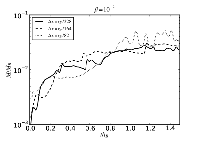
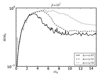
Figure 9: Convergence properties of the accretion rate of selected models as a function of time.

We find that the late time averaged accretion rates at the resolutions shown in Figure 9 exhibit asymptotic convergence with an implied order of accuracy

$$p=\frac{1}{\ln(2)}\ln\left(\frac{\dot{M}_{2x}-\dot{M}_{4x}}{\dot{M}-\dot{M}_{2x}}\right)$$ (A1)

that is better than first order accurate. In equation (A1), $\dot{M}$ is the time-averaged accretion rate at the native resolution, $\dot{M}_{2x}$ is the time-averaged accretion rate at a resolution that is coarsened by a factor of 2 and $\dot{M}_{4x}$ is the time-averaged accretion rate at a resolution that is coarsened by a factor of 4. Given the shock-capturing nature of the RAMSES code, we cannot guarantee that better than first order convergence would continue at even higher resolution. We therefore estimate the numerical grid convergence error using Richardson-extrapolation under the conservative assumption of a first order rate of convergence as

$$\epsilon=\left|\frac{\dot{M}-\dot{M}_{2x}}{\dot{M}}\right|$$ (A2)

In Table 3 summarizes the convergence properties for each of the models considered in this section. We find that the time-averaged accretion rates given by our native resolution numerical models are accurate to within $14\%$ of the Richardson-extrapolation estimate of the asymptotically converged result.

Table 3: Convergence Properties.

$\beta$	$\dot{M}_{4x}$	$\dot{M}_{2x}$	$\dot{M}$	$p$	$\epsilon$
100	0.0513	0.0400	0.0351	1.20	0.14
0.01	0.0380	0.0258	0.0243	2.46	0.062

Appendix B Bondi Flow with a Weak Magnetic Field

B.1 Dynamics

Here we calculate Bondi flow under the assumption that the gas density is initially uniform and then evolves into a steady state. This initial condition corresponds to that in our numerical simulations, but would be difficult to realize in practice (for example, an approximation to this situation might result when gas flowing supersonically past an object is suddenly brought to rest by a strong shock). We assume that the magnetic field is weak so that it does not affect the flow. As we shall see below, this approximation breaks down sufficiently close to the central mass or at sufficiently late times. The flow is then spherically symmetric, and in a steady state the accretion rate is

$$\dot{M}=4\pi\lambda{r_{\rm B}}^{2}\rho_{\infty}c,$$ (B1)

where

$${r_{\rm B}}\equiv\frac{GM_{*}}{c^{2}}$$ (B2)

is the Bondi radius associated with a star of mass $M_{*}$ and $\lambda\simeq 1.1$ for isothermal flow. For a steady accretion flow, we then have

$$4\pi r^{2}\rho v=4\pi{r_{\rm B}}^{2}\rho_{\infty}c.$$ (B3)

At large radii ($r\gg{r_{\rm B}}$), we have $\rho\simeq\rho_{\infty}$ so that

$$\frac{v}{c}\simeq\frac{{r_{\rm B}}^{2}}{r^{2}}.$$ (B4)

Henceforth, we shall normalize lengths to ${r_{\rm B}}$, velocities to $c$, and times to ${r_{\rm B}}/c$; equation (B4) then becomes $v=r^{-2}$. If we assume that the mass element is initially at rest at $r_{0}$, then at small radii or at early times, the gas is in free fall, so that

$$v=\surd 2\left(\frac{1}{r}-\frac{1}{r_{0}}\right)^{1/2}.$$ (B5)

An approximation for the flow everywhere is

$$\frac{1}{v}\simeq\frac{1}{\surd 2}\left(\frac{1}{r}-\frac{1}{r_{0}}\right)^{-1/2}+r^{2}.$$ (B6)

It should be noted that, although we used the approximation of steady flow to estimate the velocity at large radii, equation (B6) for the velocity is time dependent: $r_{0}$ is a function of both $r$ and $t$, so $\partial v/\partial t\neq 0$. In equation (B15) below we shall give the time-dependent result for Bondi flow that occurs in an initially stationary medium.

How long does it take a particle to reach a point $r$ when it starts at $r_{0}$? Integration of equation (B6) gives

$$t = \int_{r}^{r_{0}}\frac{dr}{v},$$ (B7)

$$= \frac{r_{0}^{3/2}}{\surd 2}\left\{\left[x(1-x)\right]^{1/2}+\arctan\left(\frac{1-x}{x}\right)^{1/2}\right\}+\frac{1}{3}r_{0}^{3}(1-x^{3}),$$ (B8)

where $x\equiv r/r_{0}$. The time at which the gas is accreted at the origin ($x=0$) is

$$t_{a}=\left(\frac{\pi}{2^{3/2}}\right)r_{0}^{3/2}+\frac{1}{3}r_{0}^{3}\,.$$ (B9)

Note that this result is approximate, since it depends on the harmonic mean approximation in equation (B6). We have found better agreement with the numerical results if we approximate $t_{a}$ as the root mean square of the two terms in equation (B9):

$$t_{a}=\left(\frac{\pi^{2}}{8}\,r_{0}^{3}+\frac{1}{9}\,r_{0}^{6}\right)^{1/2}.$$ (B10)

The solution of this equation shows that gas accreting at time $t$ originated from a radius $r_{0a}$ given by

$$r_{0a}^{3}=\left(\frac{9\pi^{2}}{16}\right)\frac{\tau^{2}}{1+(1+\tau^{2})^{1/2}},$$ (B11)

where

$$\tau\equiv\left(\frac{16}{3\pi^{2}}\right)t=0.540\,t.$$ (B12)

For late times ($t\gg 1$), this reduces to

$$r_{0a}\rightarrow(3t)^{1/3}.$$ (B13)

The accretion rate onto the origin is

$$\dot{M}=4\pi\lambda r_{0a}^{2}\rho_{\infty}\,\frac{dr_{0a}}{dt}~{}\times~{}{r_{\rm B}}^{2}c,$$ (B14)

where the final factor gives $\dot{M}$ the correct dimensions. Evaluating the time derivative from equation (B11), we obtain an approximation for the time-dependent accretion rate,

$$\dot{M}(t)\simeq 4\pi{r_{\rm B}}^{2}\rho_{\infty}c\;\frac{\tau}{\left(1+\tau^{2}\right)^{1/2}}.$$ (B15)

Thus, at early times the accretion rate increases linearly with time, whereas at late times it approaches the steady state value given in equation (B1) (although here we have set $\lambda=1$).

Consider now the particular case of steady flow. Since the initial location of a mass element, $r_{0}$, depends on both $r$ and $t$, the steady flow approximation is valid only if the $r_{0}^{-1}$ term in equation (B6) is negligible. This is true for $r\ll r_{0}$ or for sufficiently large $r_{0}$ provided $r$ is not too close to $r_{0}$. As a check on the accuracy of equation (B6) in this case (i.e., when $r_{0}^{-1}$ is negligible), note that the actual sonic point is at ${r_{\rm B}}/2$ (Shapiro & Teukolsky, 1983), whereas equation (B6) gives $0.65{r_{\rm B}}$; the approximation is thus accurate to within about 30%. Equation (B3) gives the density for a steady flow, which requires that the $r_{0}^{-1}$ term in equation (B6) be negligible:

$$\frac{\rho}{\rho_{\infty}}=\frac{1}{vr^{2}}\simeq 1+\frac{1}{\surd 2r^{3/2}}~{}~{}~{}~{}~{}\mbox{(steady flow)}.$$ (B16)

B.2 The Magnetic Field

When gas accretes onto the central object, both its mass and its pressure are removed from the ambient medium. In the case of the magnetic field, we assume that the flux is not accreted by the central star. As a result, the flux associated with the accreted matter, $\Phi_{a}$, builds up and distorts the flow close to the central object. When a flux tube loses mass, it becomes buoyant and drives an interchange instability. However, gas continues to accrete along this flux tube so it may eventually fall back to the center. We therefore expect that the innermost region will become turbulent. We begin with a discussion of the magnetic field in the absence of the effects of the accretion flux, and then estimate its effect at the end.

B.2.1 The Field in Smooth Inflow

Just as the gravitational force due to the star becomes important at radii less than the Bondi radius, ${r_{\rm B}}$, in the hydrodynamic case, so we expect it to become important at radii less than the Alfv$\acute{\rm e}$n-Bondi radius,

$$r_{\rm AB} \equiv \frac{GM_{*}}{v_{\rm A}^{2}}=\frac{4\pi GM_{*}\rho_{\infty}}{B_{0}^{2}},$$ (B17)

$$= 3.32\times 10^{15}\frac{M_{*}/M_{\odot}}{(v_{\rm A}/2\;\mbox{km s${}^{-1}$})^{2}}~{}~{}~{}~{}\mbox{cm}$$ (B18)

in the MHD case. The ratio of the Alfv$\acute{\rm e}$n-Bondi radius to the standard Bondi radius is

$$\frac{r_{\rm AB}}{{r_{\rm B}}}=\frac{c^{2}}{v_{\rm A}^{2}}=\frac{1}{2}\,\beta,$$ (B19)

where $\beta\equiv 8\pi\rho_{\infty}c^{2}/B_{0}^{2}$ is the plasma $\beta$. Our assumption that the field is weak implies $\beta\gg 1$. There is an important relation between $r_{\rm AB}$ and the magnetic critical mass

$$M_{\Phi}=\frac{\Phi}{2\pi G^{1/2}},$$ (B20)

which also determines the relative importance of self-gravity and magnetic fields:

$$\frac{r_{\rm AB}}{r_{0}}=\frac{4\pi GM_{*}\rho_{\infty}}{r_{0}B_{0}^{2}}=\frac{3}{4}\left(\frac{M_{0}M_{*}}{M_{\Phi}^{2}}\right),$$ (B21)

where $M_{0}=4\pi\rho_{\infty}r_{0}^{3}/3$. The magnetic field is dominant for $r_{0}>r_{\rm AB}$. In the purely gaseous case, the mass is subcritical for $M_{0}<M_{\Phi}$; in the Bondi case, we see that the gas mass $M_{0}$ is replaced by the geometric mean of the gas mass and the stellar mass (ignoring the factor $\frac{3}{4}$). Shu, Li, & Allen (2004) obtained a similar result for the case in which the gas is in a disk; they showed that it was possible for the field to be so strong that it could “levitate” the gas above a star in the process of formation. Note that the fact that it is the geometric mean mass that determines whether the gas is sub- or super-critical has an important consequence: in the purely gaseous case, a sufficiently large uniform cloud is always supercritical, since $M_{0}\propto r_{0}^{3}$ and $\Phi\propto r_{0}^{2}$. However, in the Bondi case, the opposite occurs: a sufficiently large cloud is always subcritical, since now $(M_{0}M_{*})^{1/2}\propto r_{0}^{3/2}$ increases more slowly than $\Phi$.

We assume that the field is initially uniform, so that $B_{\phi 0}=0$; for spherical inflow, $B_{\phi}$ will remain zero. For a spherical inflow, the radial flux through any surface $r^{2}d\Omega$ remains constant, so that

$$r^{2}B_{r}d\Omega=r_{0}^{2}B_{r0}d\Omega,$$ (B22)

which implies

$$B_{r}=B_{r0}\left(\frac{r_{0}}{r}\right)^{2}=B_{0}\cos\theta\left(\frac{r_{0}}{r}\right)^{2}.$$ (B23)

To evaluate $B_{\theta}$, consider a spherical shell of thickness $dr$ and radius $r$. The flux in the shell at $\theta$ is proportional to $B_{\theta}rdr$. The mass in the shell is $4\pi r^{2}\rho dr$. Since each of these remains constant in the inflow, we have

$$rB_{\theta}dr\propto\rho r^{2}dr,$$ (B24)

which implies

$$B_{\theta}=B_{\theta 0}\left(\frac{\rho r}{\rho_{\infty}r_{0}}\right)=-B_{0}\sin\theta\left(\frac{\rho r}{\rho_{\infty}r_{0}}\right),$$ (B25)

where the sign corresponds to the case in which the initial field is ${\bf B}_{0}=B_{0}\hat{\bf z}$.

How does the magnetic force compare with the gravitational one? First, we note that the radial field by itself exerts no force; we therefore consider the pressure exerted by $B_{\theta}$ and the tension force. We consider times late enough so that $r_{t}\simeq(3t)^{1/3}$ and thus that $r_{0}$ is approximately independent of $r$. For the pressure force, the relative importance of the magnetic field and gravity in the midplane ($\theta=\pi/2$) can be assessed from the ratio

$$\frac{v_{\rm A}^{2}}{v_{\rm K}^{2}}=\frac{B_{\theta}^{2}r}{4\pi\rho GM}=\left(\frac{\rho}{\rho_{\infty}}\right)\frac{r^{3}}{r_{\rm AB}r_{0}^{2}}.$$ (B26)

At large radii, we have $\rho\simeq\rho_{\infty}$; initially ($r\simeq r_{0}$) the magnetic field dominates for $r>r_{\rm AB}$, as expected. At small radii, $\rho/\rho_{\infty}\propto r^{-3/2}$ so that magnetic effects $\propto v_{\rm A}^{2}/v_{\rm K}^{2}\propto r^{3/2}$ become negligible.

Next consider the tension in the radial direction,

$$\frac{1}{4\pi}\;({\bf B}\cdot\raise 1.93747pt\hbox{$\bigtriangledown$\hskip-8.62224pt$\bigtriangledown$\hskip-8.62224pt$\bigtriangledown$\hskip-8.62224pt}\raise 2.0236pt\hbox{$\bigtriangledown$}{\bf B})_{r}=\frac{1}{4\pi}\left(\frac{B_{\theta}}{r}\,{{\partial B_{r}}\over{\partial\theta}}-\frac{B_{\theta}^{2}}{r}\right).$$ (B27)

The ratio of this force in the midplane to the gravitational force is

$$\frac{F_{\rm tension}}{F_{g}}=\frac{({\bf B}\cdot\raise 1.93747pt\hbox{$\bigtriangledown$\hskip-8.62224pt$\bigtriangledown$\hskip-8.62224pt$\bigtriangledown$\hskip-8.62224pt}\raise 2.0236pt\hbox{$\bigtriangledown$}{\bf B})_{r}}{4\pi GM\rho/r^{2}} = \frac{r_{0}}{r_{\rm AB}}\left(1-\frac{\rho r^{3}}{\rho_{\infty}r_{0}^{3}}\right)$$ (B28)

$$\rightarrow \frac{r_{0}}{r_{\rm AB}}\left[1-\frac{r^{3}}{r_{0}^{3}}\left(1+\frac{1}{\surd 2r^{3/2}}\right)\right],$$ (B29)

where the last expression applies to steady flows. Provided $r_{0}\lower 2.15277pt\hbox{$\;\buildrel>\over{\sim}\;$}1$, the density dependent term becomes negligible for $r\ll r_{0}$, so that in this case the force ratio becomes

$$\frac{F_{\rm tension}}{F_{g}}\simeq\frac{r_{0}}{r_{\rm AB}}.$$ (B30)

Since $r_{0}\simeq(3t)^{1/3}$ at late times (eq. B13), it follows that the tension force will eventually dominate and render the accretion anisotropic at

$$t_{\rm anis}\simeq\frac{r_{\rm AB}^{3}}{3c{r_{\rm B}}^{2}}=\frac{{r_{\rm B}}}{3c}\left(\frac{\beta}{2}\right)^{3},$$ (B31)

where we have explicitly included the factors of ${r_{\rm B}}$ and $c$. This is to be expected, since as noted above a sufficiently large cloud is subcritical.

B.2.2 Effects of the Accretion Flux

The accretion flux, $\Phi_{a}$, is the magnetic flux associated with the mass that has accreted onto the central mass. We expect this flux to be buoyant and to therefore lead to turbulence. Here we estimate the size of region affected by the accretion flux.

At a time $t$, the accretion flux is the flux inside the initial radius $r_{0a}$ given in equation (B11),

$$\frac{\Phi_{a}}{\pi{r_{\rm B}}^{2}B_{0}}=r_{0a}^{2}=\left(\frac{9\pi^{2}}{16}\right)^{2/3}\frac{\tau^{4/3}}{\left[1+(1+\tau^{2})^{1/2}\right]^{2/3}},$$ (B32)

We estimate the radius, $r_{\Phi}$, out to which this flux extends by assuming that the field associated with $\Phi_{a}$ is uniform, and that the flow at $r_{\Phi}$ is steady. The latter assumption requires that $r_{\Phi}$ be small compared to the starting radius, $r_{0}$, since as discussed below equation (B6), $r_{0}(r,t)$ introduces time dependent effects. We consider two limiting cases: (1) $r_{\Phi}\ll 1$, where the accretion flux interacts with supersonic inflow and (2) $r_{\Phi}>1$, where the accretion flux interacts with the pressure in the ambient medium.

Case 1: Supersonic inflow (early and intermediate times): We estimate $r_{\Phi,\,1}$, the value of $r_{\Phi}$ in this case, by determining where the pressure due to the accretion field balances the ram pressure of the accreting gas. Since we are assuming that $r_{\Phi,\,1}\ll 1$ and $r_{\Phi,\,1}\ll r_{0}$, equations (B6) and (B16) imply

$$\frac{B_{a}^{2}}{8\pi}=\rho v^{2}=\frac{\surd 2\rho_{\infty}c^{2}}{r_{\Phi,\,1}^{5/2}}$$ (B33)

Flux conservation implies $B_{a}r_{\Phi,\,1}^{2}=B_{0}r_{0a}^{2}$, so that

$$r_{\Phi,\,1} = \frac{r_{0a}^{8/3}}{2^{1/3}\beta^{2/3}},$$ (B34)

$$= \frac{1}{2^{1/3}\beta^{2/3}}\left(\frac{9\pi^{2}}{16}\right)^{8/9}\frac{\tau^{16/9}}{\left[1+(1+\tau^{2})^{1/2}\right]^{8/9}}\,.$$ (B35)

This expression is valid for both $\tau<1$ (early times) and $\tau>1$ (intermediate times). At late times, the flow is dominated by thermal pressure.

Case 2: Pressure-confined flow (late times): In this case the magnetic pressure associated with the accretion flux balances the thermal pressure of the ambient medium,

$$\frac{B_{a}^{2}}{8\pi}=\rho_{\infty}c^{2}~{}~{}\Rightarrow~{}~{}\frac{B_{a}}{B_{0}}=\beta^{1/2}.$$ (B36)

Flux conservation then implies

$$r_{\Phi,\,2} = \frac{r_{0a}}{\beta^{1/4}},$$ (B37)

$$= \frac{1}{\beta^{1/4}}\left(\frac{9\pi^{2}}{16}\right)^{1/3}\frac{\tau^{2/3}}{\left[1+(1+\tau^{2})^{1/2}\right]^{1/3}}.$$ (B38)

In order to obtain an approximation valid at all times, we write

$$\frac{1}{r_{\Phi}}\simeq\frac{1}{r_{\Phi,\,1}}\left(1+\frac{r_{\Phi,\,1}^{2}}{r_{\Phi,\,2}^{2}}\right)^{1/2}.$$ (B39)

Note that $r_{\Phi}$ is less than either $r_{\Phi,1}$ or , $r_{\Phi,2}$ corresponding to the fact that in this simple model the pressure due to the escaped flux has to balance both the thermal pressure and the ram pressure. Since $r_{\Phi,\,1}^{2}/r_{\Phi,\,2}^{2}$ exceeds unity only at late times, this can be approximated as

$$r_{\Phi}\simeq\frac{3.6\tau^{16/9}}{\beta^{2/3}\left[1+(1+\tau^{2})^{1/2}\right]^{8/9}}\cdot\frac{1}{\left(1+4.0\beta^{-5/6}\tau^{10/9}\right)^{1/2}}\,.$$ (B40)

At early times, $r_{\Phi}\propto\tau^{16/9}$; at intermediate times ($1\ll\tau\ll 0.3\beta^{3/4}$), $r_{\Phi}\propto\tau^{8/9}$; and at late times $r_{\Phi}\propto\tau^{1/3}$.

Appendix C Magnetic Bondi Flow in a Strong Magnetic Field

C.1 Initial Transient

A striking feature of Figure 2 for strong fields is that the flow is isotropic beyond some radius, but then predominantly aligned along the axis inside that, until the flow is very close to the center. This makes sense, since initially the field is straight and therefore exerts no force; thus, at sufficiently early times, the flow for a strong field is almost identical to that for no field. We focus on the region inside ${r_{\rm B}}$, where we neglect pressure forces. Let $r=r_{0}-\delta$, where $\delta\ll r_{0}$ since we are considering early times. Then equation (B5) implies

$$v=\frac{d\delta}{dt}=c\left(\frac{2{r_{\rm B}}\delta}{rr_{0}}\right)^{1/2}\simeq c\,\frac{(2{r_{\rm B}}\delta)^{1/2}}{r_{0}},$$ (C1)

where we have written the equation in dimensional form. Integration gives

$$\delta=\frac{{r_{\rm B}}c^{2}t^{2}}{2r_{0}^{2}}.$$ (C2)

The ratio of the tension force to the gravitational force at early times is given by equation (B28) with $\rho=\rho_{0}$. For small $\delta$, this is

$$\frac{F_{t}}{F_{g}}=\frac{3\delta}{r_{\rm AB}}.$$ (C3)

The magnetic field will begin deflecting the flow from a radial trajectory to an axial one when this ratio is of order unity, which occurs at

$$\frac{r_{0}}{{r_{\rm B}}}=\left(\frac{3}{\beta}\right)^{1/2}\frac{t}{{t_{\rm B}}}.$$ (C4)

We have found that the growth of the region deflected from a radial trajectory in our numerical simulations with $\beta=0.1$ and $\beta=0.01$ follow this functional form very well but that the deflection from spherical flow occurs somewhat later than predicted. We extract a good empirical fit to the low-$\beta$ simulations with

$$\frac{r_{0}}{{r_{\rm B}}}=\left(\frac{2.0}{\beta}\right)^{1/2}\frac{t}{{t_{\rm B}}}.$$ (C5)

C.2 Magnetic Bondi Flow in a Strong Magnetic Field ($\beta\lower 2.15277pt\hbox{$\;\buildrel<\over{\sim}\;$}0.1$) at Late Times

For a very strong field, the gas will attempt to settle into vertical hydrostatic equilibrium,

$$\rho=\rho_{\infty}e^{-m\phi/kT}=\rho_{\infty}e^{{r_{\rm B}}/r}$$ (C6)

where $m$ is the mass per particle and $\phi=-GM_{*}/r$ is the gravitational potential. Henceforth, we shall normalize all lengths to the Bondi radius, as in the previous section. Outside the Bondi radius, this expression gives only a modest increase in density, but for small radii the increase can be very large–so large that it takes a long time to reach equilibrium. Let $\varpi$ be the cylindrical radius, so that $r=(\varpi^{2}+z^{2})^{1/2}$, where $z$ is the height above the disk. The density at the midplane ($r=\varpi$) is then

$$\rho_{0}=\rho_{\infty}e^{1/\varpi}.$$ (C7)

For small radii, $\varpi\ll 1$, the density distribution near the midplane is approximately gaussian,

$$\rho\simeq\rho_{0}e^{-z^{2}/h^{2}},$$ (C8)

where $\rho_{0}$ is the midplane density and the scale height is

$$h=\surd 2\varpi^{3/2}.$$ (C9)

In equilibrium, the total surface density of the gas near the midplane is then

$$\Sigma_{\rm eq}\simeq 2\rho_{0}h=\rho_{\infty}{r_{\rm B}}(2\varpi)^{3/2}e^{1/\varpi},$$ (C10)

where we have used equation (C7) to eliminate $\rho_{0}$.

When do magnetic forces balance gravity? For a thin disk, magnetic tension dominates magnetic pressure (Shu & Li, 1997). For an axisymmetric field, the net radial tension is

$$F_{t}=\frac{1}{4\pi}({\bf B}\cdot\raise 1.93747pt\hbox{$\bigtriangledown$\hskip-8.62224pt$\bigtriangledown$\hskip-8.62224pt$\bigtriangledown$\hskip-8.62224pt}\raise 2.0236pt\hbox{$\bigtriangledown$})B_{\varpi}=\frac{1}{4\pi{r_{\rm B}}}B_{z}{{\partial B_{\varpi}}\over{\partial z}}.$$ (C11)

Integrating through the disk, we find that the forces balance when

$$\frac{1}{4\pi}B_{z}(2B_{\varpi})=\frac{GM_{*}\Sigma}{{r_{\rm B}}\varpi^{2}},$$ (C12)

where $B_{\varpi}$ is measured just above the disk.

To obtain an accurate solution beyond this point, we would have to solve for the structure of the field. This is a challenging problem even when the system is in equilibrium. Here, however, we are assuming that the system is in equililbrium outside some critical radius, $\varpi_{\rm cr}$, but that there is an unknown accretion flow inside that radius. We therefore content ourselves with attemping to infer the scaling for the solution. We assume that $B_{z}$ in the disk is proportional to the ambient field, $B_{\infty}$, and that the radial component of the field, $B_{\varpi}$, is proportional to $B_{z}$. Equation (C12) then implies that

$$\Sigma\sim\rho_{\infty}{r_{\rm B}}\left(\frac{\varpi^{2}}{\beta}\right).$$ (C13)

For a given location in the disk, gas will accrete along the field lines until the surface density reaches this value. The field is unable to support more gas than this, so this value represents an upper limit on $\Sigma$; any additional gas will accrete onto the central star. However, we have determined another maximum value for the surface density in equation (C10), which is the value the surface density has in hydrostatic equilibrium. Equating these two surface densities determines the critical radius, $\varpi_{\rm cr}$: The gas can be supported by the field outside $\varpi_{\rm cr}$, but inside $\varpi_{\rm cr}$ gas that exceeds the surface density in equation (C13) must fall onto the central star. Equations (C10) and (C13) imply that this critical radius satisfies

$$\varpi_{\rm cr}^{1/2}e^{-1/\varpi_{\rm cr}}\sim\beta.$$ (C14)

A good approximation for the solution of this equation for $\beta\lower 2.15277pt\hbox{$\;\buildrel<\over{\sim}\;$}0.15$, corresponding to $\varpi_{\rm cr}\lower 2.15277pt\hbox{$\;\buildrel<\over{\sim}\;$}0.6$, is

$$\varpi_{\rm cr}\simeq\frac{1}{\ln\beta^{-1}-0.5\ln\ln\beta^{-1}}~{}~{}~{}~{}~{}~{}~{}~{}(\beta\lower 2.15277pt\hbox{$\;\buildrel<\over{\sim}\;$}0.15).$$ (C15)

In the regime of greatest interest, $10^{-3}<\beta<0.15$, the solution can be approximated by the simpler form

$$\varpi_{\rm cr}\simeq 0.85\beta^{1/4}~{}~{}~{}~{}~{}~{}~{}~{}~{}~{}~{}~{}~{}(10^{-3}\lower 2.15277pt\hbox{$\;\buildrel<\over{\sim}\;$}\beta\lower 2.15277pt\hbox{$\;\buildrel<\over{\sim}\;$}0.15).$$ (C16)

The accuracy of this solution in the prescribed range is about 10%, which is much better than the accuracy of the underlying equation.

We are now in a position to estimate the accretion rate onto the central star. We assume that the accretion flow is primarily along the field lines, and that it is initiated by a rarefaction wave propagating at the sound speed, $c$. After an initial phase during which the surface density just inside $\varpi_{\rm cr}$ becomes large enough that it distorts the field so much that it can accrete, the accretion rate on both sides of the disk becomes

$$\dot{M}\simeq 2(\pi{r_{\rm B}}^{2}\varpi_{\infty,\,\rm cr}^{2})\rho_{\infty}c,$$ (C17)

where $\varpi_{\infty,\,\rm cr}$ is the cylindrical radius of the critical field lines far from the star. If we assume that $\varpi_{\rm cr}\propto\varpi_{\infty,\,\rm cr}$, then in the range $10^{-3}\lower 2.15277pt\hbox{$\;\buildrel<\over{\sim}\;$}\beta\lower 2.15277pt\hbox{$\;\buildrel<\over{\sim}\;$}0.1$ we have $\dot{M}\propto\varpi_{\rm cr}^{2}\propto\beta^{1/2}$, and we can write

$$\dot{M}=4\pi\lambda_{\rm low\;\beta}{r_{\rm B}}^{2}\rho_{\infty}c\beta^{1/2},$$ (C18)

where $\lambda_{\rm low\;\beta}$ is a numerical constant. Note that the $\beta^{1/2}$ scaling is the same as that implied by the crude argument in the text. Were we to assume that $\varpi_{\infty,\,\rm cr}=\varpi_{\rm cr}$ and that equation (C16) were accurate, then $\lambda_{\rm low\;\beta}$ would equal 0.36. This estimate is within a factor 1.6 of the numerical results. Setting $\lambda_{\rm low\;\beta}=0.24$ gives an accretion rate that agrees with the results of the simulations for $\beta=0.1,\,0.01$ to within 8%.

References

- Bate et al. (1995) Bate, M. R., Bonnell, I. A., & Price, N. M. 1995, MNRAS, 277, 362
- Bernstein et al. (1958) Bernstein, I. B., Frieman, E. A., Kruskal, M. D., & Kulsrud, R. M. 1958, Royal Society of London Proceedings Series A, 244, 17
- Bondi (1952) Bondi, H. 1952, MNRAS, 112, 195
- Bondi & Hoyle (1944) Bondi, H., & Hoyle, F. 1944, MNRAS, 104, 273
- Bonnell et al. (1997) Bonnell, I. A., Bate, M. R., Clarke, C. J., & Pringle, J. E. 1997, MNRAS, 285, 201
- Crutcher (1999) Crutcher, R. M. 1999, ApJ, 520, 706
- Federrath et al. (2010) Federrath, C., Banerjee, R., Clark, P. C., & Klessen, R. S. 2010, ApJ, 713, 269
- Furth et al. (1963) Furth, H. P., Killeen, J., & Rosenbluth, M. N. 1963, Physics of Fluids, 6, 459
- Igumenshchev & Narayan (2002) Igumenshchev, I. V., & Narayan, R. 2002, ApJ, 566, 137
- Igumenshchev (2006) Igumenshchev, I. V. 2006, ApJ, 649, 361
- Krumholz et al. (2007) Krumholz, M. R., Klein, R. I., & McKee, C. F. 2007, ApJ, 656, 959
- Krumholz et al. (2004) Krumholz, M. R., McKee, C. F., & Klein, R. I. 2004, ApJ, 611, 399
- Krumholz et al. (2005) Krumholz, M. R., McKee, C. F., & Klein, R. I. 2005, ApJ, 618, 757
- Krumholz et al. (2005) Krumholz, M. R., McKee, C. F., & Klein, R. I. 2005, Nature, 438, 332
- Krumholz et al. (2006) Krumholz, M. R., McKee, C. F., & Klein, R. I. 2006, ApJ, 638, 369
- Kulkarni & Romanova (2008) Kulkarni, A. K., & Romanova, M. M. 2008, MNRAS, 386, 673
- Long et al. (2011) Long, M., Romanova, M. M., Kulkarni, A. K., & Donati, J.-F. 2011, MNRAS, 413, 1061
- McKee & Ostriker (2007) McKee, C. F., & Ostriker, E. C. 2007, ARA&A, 45, 565
- Offner et al. (2009) Offner, S. S. R., Klein, R. I., McKee, C. F., & Krumholz, M. R. 2009, ApJ, 703, 131
- Padoan & Nordlund (2011) Padoan, P., & Nordlund, Å. 2011, ApJ, 730, 40
- Pang et al. (2011) Pang, B., Pen, U.-L., Matzner, C. D., Green, S. R., & Liebendörfer, M. 2011, MNRAS, 415, 1228
- Teyssier (2002) Teyssier, R. 2002, A&A, 385, 337
- Romanova et al. (2008) Romanova, M. M., Kulkarni, A. K., & Lovelace, R. V. E. 2008, ApJ, 673, L171
- Romanova et al. (2011) Romanova, M. M., Ustyugova, G. V., Koldoba, A. V., & Lovelace, R. V. E. 2011, MNRAS, 1153
- Ruffert (1994) Ruffert, M. 1994, ApJ, 427, 342
- Ruffert & Arnett (1994) Ruffert, M., & Arnett, D. 1994, ApJ, 427, 351
- Rutherford (1973) Rutherford, P. H. 1973, Physics of Fluids, 16, 1903
- Shapiro (1973) Shapiro, S. L. 1973, ApJ, 185, 69
- Shapiro & Teukolsky (1983) Shapiro, S.L., Teukolsky, S.A., 1983, Black Holes, White Dwarfs and Neutron Stars, Wiley, N.Y.
- Shcherbakov (2008) Shcherbakov, R. V. 2008, ApJS, 177, 493
- Shima et al. (1985) Shima, E., Matsuda, T., Takeda, H., & Sawada, K. 1985, MNRAS, 217, 367
- Shu (1992) Shu, F. H. 1992, The Physics of Astrophysics. Volume II: Gas dynamics., by Shu, F. H.. University Science Books, Mill Valley, CA (USA), 1992, 493 p., ISBN 0-935702-65-2
- Shu & Li (1997) Shu, F. H., & Li, Z.-Y. 1997, ApJ, 475, 251
- Toropin et al. (1999) Toropin, Y. M., Toropina, O. D., Savelyev, V. V., et al. 1999, ApJ, 517, 906
- Ustyugova et al. (2006) Ustyugova, G. V., Koldoba, A. V., Romanova, M. M., & Lovelace, R. V. E. 2006, ApJ, 646, 304
- Vázquez-Semadeni et al. (2011) Vázquez-Semadeni, E., Banerjee, R., Gómez, G. C., Hennebelle, P., Duffin, D., & Klessen, R. S. 2011, MNRAS, 414, 2511
- Wang et al. (2010) Wang, P., Li, Z.-Y., Abel, T., & Nakamura, F. 2010, ApJ, 709, 27